FUNDAÇÃO GETULIO VARGAS
ESCOLA DE ECONOMIA DE SÃO PAULO
MATHEUS PIMENTEL RODRIGUES
THE EFFECT OF DEFAULT RISK ON TRADING BOOK
CAPITAL REQUIREMENTS FOR PUBLIC EQUITIES:
AN IRC APPLICATION FOR THE BRAZILIAN MARKET
SÃO PAULO
MATHEUS PIMENTEL RODRIGUES
THE EFFECT OF DEFAULT RISK ON TRADING BOOK
CAPITAL REQUIREMENTS FOR PUBLIC EQUITIES:
AN IRC APPLICATION FOR THE BRAZILIAN
MARKET
Presented dissertation in the master’s pro-gram of the São Paulo School of Economics, member of Fundação Getúlio Vargas, as part of the requisites to obtain the title of master in Economics, with emphasis in Quantitative Finance.
Dissertation Advisor
Prof. Dr. Afonso de Campos Pinto
Pimentel Rodrigues, Matheus.
The effect of default risk on trading book capital requirements for public equities: an IRC application for the Brazilian Market / Matheus Pimentel Rodrigues - 2015.
94f.
Orientador: Afonso de Campos Pinto.
Dissertação (MPFE) - Escola de Economia de São Paulo.
1. Mercado financeiro. 2. Risco (Economia). 3. Modelos econométricos. 4. Monte Carlo, Método de. I. Pinto, Afonso de Campos. II. Dissertação (MPFE) -Escola de Economia de São Paulo. III. The effect of default risk on trading book capital requirements for public equities: an IRC application for the Brazilian Market.
MATHEUS PIMENTEL RODRIGUES
THE EFFECT OF DEFAULT RISK ON TRADING BOOK
CAPITAL REQUIREMENTS FOR PUBLIC EQUITIES:
AN IRC APPLICATION FOR THE BRAZILIAN
MARKET
Presented dissertation in the master’s pro-gram of the São Paulo School of Economics, member of Fundação Getúlio Vargas, as part of the requisites to obtain the title of master in Economics, with emphasis in Quantitative Finance.
Approval Date: 17 / 08 / 2015
Examination Board:
Prof. Dr. Afonso de Campos Pinto (Dissertation Advisor)
Fundação Getúlio Vargas
Prof. Dr. André Cury Maialy Fundação Getúlio Vargas
Agradecimentos
Acknowledgements
RESUMO
Esse é um dos primeiros trabalhos a endereçar o problema de avaliar o efeito do default
para fins de alocação de capital notrading book em ações listadas. E, mais especificamente,
para o mercado brasileiro. Esse problema surgiu em crises mais recentes e que acabaram fazendo com que os reguladores impusessem uma alocação de capital adicional para essas operações. Por essa razão o comitê de Basiléia introduziu uma nova métrica de risco, conhecida como Incremental Risk Charge.
Essa medida de risco é basicamente um VaR de um ano com um intervalo de confiança de 99.9%. O IRC visa medir o efeito do default e das migrações de rating, para instrumentos
do trading book. Nessa dissertação, o IRC está focado em ações e como consequência, não
leva em consideração o efeito da mudança de rating.
Além disso, o modelo utilizado para avaliar o risco de crédito para os emissores de ação foi o Moody’s KMV, que é baseado no modelo de Merton. O modelo foi utilizado para calcular a PD dos casos usados como exemplo nessa dissertação.
Após calcular a PD, simulei os retornos por Monte Carlo após utilizar um PCA. Essa abordagem permitiu obter os retornos correlacionados para fazer a simulação de perdas do portfolio. Nesse caso, como estamos lidando com ações, o LGD foi mantido constante e o valor utilizado foi baseado nas especificações de basiléia.
Os resultados obtidos para o IRC adaptado foram comparados com um VaR de 252 dias e com um intervalo de confiança de 99.9%. Isso permitiu concluir que o IRC é uma métrica de risco relevante e da mesma escala de uma VaR de 252 dias. Adicionalmente, o IRC adaptado foi capaz de antecipar os eventos de default. Todos os resultados foram baseados em portfolios compostos por ações do índice Bovespa.
ABSTRACT
This is one of the first works to address the issue of evaluating the effect of default for capital allocation in the trading book, in the case of public equities. And more specifically, in the Brazilian Market. This problem emerged because of recent crisis, which increased the need for regulators to impose more allocation in banking operations. For this reason, the BIS committee, recently introduce a new measure of risk, the Incremental Risk Charge.
This measure of risk, is basically a one year value-at-risk, with a 99.9% confidence level. The IRC intends to measure the effects of credit rating migrations and default, which may occur with instruments in the trading book. In this dissertation, the IRC was adapted for the equities case, by not considering the effect of credit rating migrations.
For that reason, the more adequate choice of model to evaluate credit risk was the Moody’s KMV, which is based in the Merton model. This model was used to calculate the PD for the issuers used as case tests.
After, calculating the issuer’s PD, I simulated the returns with a Monte Carlo after using a PCA. This approach permitted to obtain the correlated returns for simulating the portfolio loss. In our case, since we are dealing with stocks, the LGD was held constant and its value based in the BIS documentation.
The obtained results for the adapted IRC were compared with a 252-day VaR, with a 99% confidence level. This permitted to conclude the relevance of the IRC measure, which was in the same scale of a 252-day VaR. Additionally, the adapted IRC was capable to anticipate default events. All result were based in portfolios composed by Ibovespa index stocks.
List of Figures
Figure 1 – Structure of the Adapted IRC Model . . . 25
Figure 2 – Asset value path and distribution. . . 28
Figure 3 – Comparison between the distribution of equity returns and credit returns. 33 Figure 4 – ABEV3 Assets Behavior and Probability of Default . . . 40
Figure 5 – PETR4 Assets Behavior and Probability of Default . . . 40
Figure 6 – BRFS3 Assets Behavior and Probability of Default . . . 40
Figure 7 – CIEL3 Assets Behavior and Probability of Default. . . 40
Figure 8 – VALE5 Assets Behavior and Probability of Default . . . 41
Figure 9 – JBSS3 Assets Behavior and Probability of Default . . . 41
Figure 10 – BVMF3 Assets Behavior and Probability of Default . . . 41
Figure 11 – EMBR3 Assets Behavior and Probability of Default . . . 41
Figure 12 – KROT3 Assets Behavior and Probability of Default . . . 42
Figure 13 – VIVT4 Assets Behavior and Probability of Default . . . 42
Figure 14 – LREN3 Assets Behavior and Probability of Default . . . 42
Figure 15 – PCAR4 Assets Behavior and Probability of Default . . . 42
Figure 16 – CCRO3 Assets Behavior and Probability of Default . . . 43
Figure 17 – CMIG4 Assets Behavior and Probability of Default . . . 43
Figure 18 – CSNA3 Assets Behavior and Probability of Default . . . 43
Figure 19 – CYRE3 Assets Behavior and Probability of Default . . . 43
Figure 20 – USIM5 Assets Behavior and Probability of Default . . . 44
Figure 21 – PDGR3 Assets Behavior and Probability of Default . . . 44
Figure 22 – OGXP3 Assets Behavior and Probability of Default . . . 44
Figure 23 – MMXM3 Assets Behavior and Probability of Default . . . 44
Figure 24 – Adapted IRC vs. VaR comparison for Portfolio 1 . . . 45
Figure 25 – Weight Distribution of Portfolio 1 over time . . . 46
Figure 26 – BRKM5 Assets Behavior and Probability of Default . . . 47
Figure 27 – BRML3 Assets Behavior and Probability of Default . . . 47
Figure 28 – CESP6 Assets Behavior and Probability of Default . . . 47
Figure 29 – CPFE3 Assets Behavior and Probability of Default . . . 47
Figure 30 – CPLE6 Assets Behavior and Probability of Default . . . 48
Figure 31 – CRUZ3 Assets Behavior and Probability of Default . . . 48
Figure 32 – ENBR3 Assets Behavior and Probability of Default . . . 48
Figure 33 – ESTC3 Assets Behavior and Probability of Default . . . 48
Figure 34 – FIBR3 Assets Behavior and Probability of Default . . . 49
Figure 35 – GFSA3 Assets Behavior and Probability of Default . . . 49
Figure 37 – HGTX3 Assets Behavior and Probability of Default . . . 49
Figure 38 – HYPE3 Assets Behavior and Probability of Default . . . 50
Figure 39 – NATU3 Assets Behavior and Probability of Default . . . 50
Figure 40 – OIBR4 Assets Behavior and Probability of Default . . . 50
Figure 41 – POMO4 Assets Behavior and Probability of Default . . . 50
Figure 42 – RENT3 Assets Behavior and Probability of Default . . . 51
Figure 43 – SUZB5 Assets Behavior and Probability of Default . . . 51
Figure 44 – OGXP3 Assets Behavior and Probability of Default . . . 51
Figure 45 – TIMP3 Assets Behavior and Probability of Default . . . 51
Figure 46 – Adapted IRC vs. VaR comparison for Portfolio 2 . . . 52
Figure 47 – Weight Distribution of Portfolio 2 over time . . . 53
Figure 48 – Adapted IRC vs. VaR comparison for Portfolio 3 . . . 53
Figure 49 – PCA and Loss Distribution for Portfolio 1 in month 1 . . . 84
Figure 50 – PCA and Loss Distribution for Portfolio 1 in month 10 . . . 84
Figure 51 – PCA and Loss Distribution for Portfolio 1 in month 20 . . . 84
Figure 52 – PCA and Loss Distribution for Portfolio 1 in month 30 . . . 85
Figure 53 – PCA and Loss Distribution for Portfolio 1 in month 40 . . . 85
Figure 54 – PCA and Loss Distribution for Portfolio 1 in month 48 . . . 85
Figure 55 – PCA and Loss Distribution for Portfolio 2 in month 1 . . . 86
Figure 56 – PCA and Loss Distribution for Portfolio 2 in month 10 . . . 86
Figure 57 – PCA and Loss Distribution for Portfolio 2 in month 20 . . . 86
Figure 58 – PCA and Loss Distribution for Portfolio 2 in month 30 . . . 87
Figure 59 – PCA and Loss Distribution for Portfolio 2 in month 40 . . . 87
Figure 60 – PCA and Loss Distribution for Portfolio 2 in month 48 . . . 87
Figure 61 – PCA and Loss Distribution for Portfolio 3 in month 1 . . . 88
Figure 62 – PCA and Loss Distribution for Portfolio 3 in month 10 . . . 88
Figure 63 – PCA and Loss Distribution for Portfolio 3 in month 20 . . . 88
Figure 64 – PCA and Loss Distribution for Portfolio 3 in month 30 . . . 89
Figure 65 – PCA and Loss Distribution for Portfolio 3 in month 40 . . . 89
Figure 66 – PCA and Loss Distribution for Portfolio 3 in month 48 . . . 89
List of Tables
Table 1 – An illustration of the balance sheet structure. . . 26
Table 2 – Step 1 - Monte Carlo simulation of asset values to generate correlated loss. 31
Table 3 – Step 2 - Monte Carlo simulation of asset values to generate correlated loss. 32
Table 4 – Step 3 - Monte Carlo simulation of asset values to generate correlated loss. 32
Table 5 – Ibovespa index companies used in the first portfolio study. . . 34
List of abbreviations and acronyms
BIS Bank of International Settlements
EBA European Banking Authority
IRC Incremental Risk Charge
VaR Value-at-Risk
PRM Market Risk Parcel
PRE Required Regulatory Capital
TPM Transition Probability Matrix
PD Probability of Default
EAD Exposure at Default
LGD Loss Given Default
At Asset value at time t
Et Equity value at time t
Dt Debt value at time t
r Risk-free yield rate
T End time of period
σA Volatility of the asset
σE Volatility of the equity
µA Return of the asset
DD Distance-to-Default
Contents
1 Introduction . . . 16
1.1 Motivation . . . 16
1.2 Objectives . . . 16
2 Bibliographic Review . . . 17
2.1 Basic Concepts . . . 17
2.2 State of the art . . . 20
2.3 The present work and the literature . . . 21
3 Model Development . . . 23
3.1 The problem description . . . 23
3.2 Addressing the problem . . . 24
3.3 The Model . . . 26
3.3.1 The Merton model . . . 26
3.3.2 The Multifactor Model for Asset Returns . . . 30
3.3.3 The Portfolio Loss . . . 31
3.4 Expected Results . . . 32
4 Theory application . . . 34
4.1 Description of the case study. . . 34
4.2 Data selection . . . 35
4.2.1 KMV Moody’s - Parameter Estimation . . . 35
4.2.2 Principal component analysis - Parameter Estimation . . . 37
4.3 Application to the case . . . 37
5 Result Discussion . . . 39
6 Conclusion . . . 54
7 Future Research . . . 56
Bibliography . . . 57
APPENDIX A Matlab Code . . . 59
A.1 Adapted IRC Model . . . 59
A.2 Getdata . . . 79
A.3 Merton Model . . . 80
A.4 Portfolio Loss . . . 83
ANNEX A Trading Book Capital Requirements . . . 91
16
1 Introduction
1.1 Motivation
This dissertation was motivated by the need to study and understand the effect of default events in capital requirements in the trading book for public equities. This will be done by focusing in elements present in the Brazilian market. Moreover, this subject was originated by recent changes in regulation proposed by the Bank of International Settlements (BIS). These changes require banks to reserve capital in the trading book for credit migration and default events. This covers corporate bonds, CDS, equity and correlation products. This kind of capital charge is known as Incremental Risk Charge (IRC) and it is based on a VaR calculation using a one-year time horizon and calibrated
to a 99.9th percentile confidence level, see (SETTLEMENTS,2013a).
Banks usually do not consider the effect of credit events for capital requirements in the trading book for equity instruments, because it is difficult to establish a relation to one another. The main reason is not existing a clear link between credit rating migration and change in equity returns. Additionally, in Brazil, the regulation does not consider in the capital requirements for the trading book any risk measure similar to the IRC. As we will see, there is another difficulty for the Brazilian Market, which is the lack of liquidity in private debt instruments. To overcome these two difficulties, we will adapt the IRC measure and compare the results with typical 10-day VaR methodology with a 99th percentile confidence level.
1.2 Objectives
The main goal of this dissertation is to evaluate the effect of default to the capital allocation in the trading book, for a portfolio of public equities. Addionally, it will focus in the Brazilian Market case.
I intend to address and explore the Incremental Risk Charge, which is a risk measure for market risk. All the past work about this subject focused in debt instruments, and I will focus in equity instruments. I also intend to compare the results with the VaR measure defined for market risk in the Brazilian regulation.
17
2 Bibliographic Review
2.1 Basic Concepts
The concept of IRC was first introduced in the documentGuidelines for Computing Capital for Incremental Risk in the Trading Book, see (SETTLEMENTS, 2008) and
(SETTLEMENTS, 2009b). As described in the document, The Basel Committee/IOSCO Agreement reached in July 2005 contained several improvements to the capital regime for trading book positions. Among these revisions was a new requirement for banks that model specific risk to measure and hold capital against default risk that is incremental to any default risk captured in the bank’s 99%/10-day value-at-risk model. The first modification was the incremental default risk charge, which was incorporated into the trading book capital regime in response to the increasing amount of exposure in banks’ trading books to credit risk related and often illiquid products whose risk is not reflected in VaR. After reviewing comments about this modification, the committee decided that applying an incremental risk charge covering default risk only would not appear adequate. Because, the losses have arisen defaults, credit migrations combined with widening of credit spreads and the loss of liquidity. The IRC is intended to complement additional standards being applied to the value-at-risk modelling framework. Together, these changes address a number of perceived shortcomings in the current 99%/10-day VaR framework. Additionally, these documents set the principles for IRC calculations, such as: IRC-covered positions and Key supervisory parameters for computing IRC.
Chapter 2. Bibliographic Review 18
Basically, our objective is to model some type of credit risk. The principles for modeling this kind of risk were first addressed in (MERTON, 1974). The paper presented a systematic theory for pricing bonds when there is a significant probability of default. Furthermore, the value of a particular issue of corporate debt was characterized by depending on essentially three items: the required rate of return on riskless debt; the various provisions and restrictions contained in the indenture, e.g., maturity date, coupon rate, call terms, seniority in the event of default, sinking fund, etc.; the probability that the firm will be unable to satisfy some or all of the indenture requirements, i.e., the probability of default. The Merton paper (MERTON, 1974) clarified and extended the Black-Scholes model for option pricing, (BLACK; SCHOLES,1973). Both Black and Scholes and Merton recognized that the approach could be applied in developing a pricing theory for corporate liabilities in general. A basic equation for the pricing of financial instruments was developed in the paper, the model was applied to the simplest form of corporate debt, the discount bond where no coupon payments are made, and a formula for computing the risk structure of interest rates was presented.
The Merton model permitted the development of several methodologies for modeling default risk. These methodologies based on the Merton model are called structural models. One of the most known structural model is the Moody’s KMV, see (BOHN; CROSBIE,
Chapter 2. Bibliographic Review 19
is a marginally useful default forecaster, but it is not a sufficient statistic for default. Moreover, both papers acknowledged that their implementation of the KMV-Merton model is different from that of Moody’s KMV, and therefore the forecasts of Moody’s KMV might be better than those tested in this paper. The third is a much simpler paper which only describes the methodology and then emphasizes the importance of the KMV model as one more possible tool to asses credit risk.
Another methodology, based on a structural model is the CreditMetrics, see (GUPTON; FINGER; BHATIA, 1997). CreditMetrics is a tool for assessing portfolio risk due changes in obligor credit quality, including changes in value caused not only by possible default events, but also by upgrades and downgrades in credit quality. More importantly, it measures the VaR due to credit quality changes. Also, the model addresses the correlation of credit quality moves across obligors. This allows to directly calculate the diversification benefits or potential over-concentrations across a portfolio.
Chapter 2. Bibliographic Review 20
VICENTE, 2013), the authors also present the Nelson-Siegel methodology to build the yield curve for a certain rating class. They used this methodology for the few existing rating classes and built the curves for these ratings.
2.2 State of the art
Many thesis and papers focus on developing an IRC model, one example of work based on this subject is (FORSMAN, 2012). The task of that thesis was to develop an IRC model for a portfolio of simple corporate bonds in accordance with the guidelines of the Basel 3 Committee. The aim was to develop an elementary model for IRC that yields a reasonable result and to analyze the effect on calculated risk using various model specifications, in particular the effects of liquidity horizons, credit spreads, correlations and transition probabilities. The model assumes a constant level of risk, thus each position in the portfolio is rebalanced (replacing the position with the initial position) either if the liquidity horizon of that position is reached or if a default has occurred. The author emphasizes that extending the model to cover other positions, besides bonds, should not be difficult to make as long as the positions can be evaluated by their credit quality. By stress testing the model, the author shows that the default risk accounts for a greater part of the risk than the migration risk. An interesting finding was the nearly perfect linear relationship between the recovery rate and the VaR. The VaR also varies a lot depending on the correlations among the different issuers in the portfolio. About the liquidity horizon, the author shows that it was not self-explanatory how the specific length of this affects the risk. Small changes in the liquidity horizons did not seem to have a significant impact on the VaR in the model. The reason for this was that by increasing the horizon, the default risk was raised but the migration risk was decreased slightly. Therefore, the total change in VaR caused by longer liquidity horizons became almost negligible. Finally, the author found out that changes in the credit spreads affected the risk in two ways. If the gaps between the spreads increase or if the whole credit spread curve rises at some point during the simulation the potential loss rises.
Chapter 2. Bibliographic Review 21
how to allocate the liquidity horizons across different credit grades by minimizing the IRC add-on.
A third paper about IRC is (YAVIN et al., 2014). The focus of this paper is about the methodology for building a transition probability matrix (TPM), since to model IRC is necessary modeling default and migration with a period shorter than one year. The paper divides the estimation of TPMs in two problems. First, finding an appropriate one-year TPM with predefined sectors and ratings. Second, both Basel PDs and rating agencies TPMs are annual but the TPM we need is one with a term shorter than one year, typically it has to be monthly or quarterly, depending on the time step in the IRC simulation engine. Given the statistical nature of TPMs and Basel PDs, it is not a trivial task to achieve this. It is worth noting that TPMs play a crucial role in the IRC simulation methodology. The paper than summarizes most of the exercise to compute TPMs for IRC, emphasizing the large uncertainties in the computed TPMs. The author refrained from making specific recommendations on which method performs best, due to varying portfolio composition among different institutions. Therefore, the author concludes that given the importance of TPMs and their PDs in the IRC, financial institutions will need to make discretionary choices regarding their preferred methodology while ensuring that uncertainties are well understood, managed and communicated properly to local regulators.
The fourth and the most extensive thesis about IRC is (STEL, 2010). The author begins by describing the CreditMetrics model and the need to modify it to attend the Basel Committee’s modelling requirements. He divided the study in three parts: first, the requirements and principles of the model were discussed so a complete model could be derived in terms of a simulation model and a correlation structure; second, the estimation of the required inputs in the derived model; third, the assessment of the model and its inputs and assumptions. The conclusion is that the copula assumption, the assumed lengths of the liquidity horizons of the assessed positions, the applied conditionality in credit migration matrix and the average level of issuer asset correlations in the model are crucial inputs in the estimation of the required risk measure in any IRC model. On the other hand, the precision of the issuer correlations and the choice in the methodology utilized in the estimation of the credit migration matrix that is applied in the model in the model seems to be much less crucial.
2.3 The present work and the literature
Since the IRC was established by the Basel Committee, the BIS tried to evaluate the impact of this risk measure, by consulting the banks which implemented the model, or even, by evaluating the impact of not implementing it. The document, (SETTLEMENTS,
Chapter 2. Bibliographic Review 22
implemented the IRC. Of the 25 banks, three included equity exposures into their IRC model. The study showed that the net effect of the IRC is estimated to result in an average increase of 103% in market risk capital. The bank-level results indicated that the IRC produced a net increase in market risk capital for all but two banks. On the other hand, the paper (SETTLEMENTS, 2013b), also from the BIS, indicated that Brazilian banks opting for using internal models are required under the Brazilian regulations to develop a VaR but not an IRC model. As a result, Brazilian banks using internal models developed a VaR model and used the standardized approach to capture the specific risk of their trading book. This approach is more conservative in the Brazilian Regulation, but this is not true for the Basel approach. Particularly, for the Brazilian case, the a BIS assessment team understood that the kind of exposition on the Brazilian trading books would not demand much more capital, since these banks are more exposed to sovereign bonds. Thus, it was considered compliant.
The Brazilian Regulation for capital requirements in the trading book is better described in the dissertation (VIEIRA; FILHO, 2012). As described in that dissertation, the Brazilian Central Bank released in 2012 the Circular number 3498 which introduced in the capital for market risk the component of stressed VaR, but it did not introduce the component of the IRC. Meaning that, the PRM (component of market risk in the required capital, PRE) does not consider the risk of default for equities. Thus, Brazilian banks do not calculate the IRC for equities, what some do is allocate capital for credit risk to compensate for not allocating capital for market risk due to default in equities.
Since the papers, (FORSMAN,2012), (SKOGLUND; CHEN,2010), (YAVIN et al.,
23
3 Model Development
3.1 The problem description
To compute the effect of default in the capital requirements of the trading book for equities, first we examine the latest release of the IRC measures by the Basel Com-mittee. This section will describe the most relevant aspects as presented in Guidelines for Computing Capital for Incremental Risk in the Trading Book: Consultative Document (SETTLEMENTS, 2009b) and (SETTLEMENTS, 2008). The guidelines presented in that document set forth the requirements and principles to which IRC model must comply. Additionally, we address the particularities demanded to adapt the measure for Brazilian public equities.
The IRC must capture the migration and default risk to the positions in the trading book of a bank, see (SETTLEMENTS,2009b). The IRC encompasses all positions subject to a capital charge for specific interest rate risk according to the internal models approach to specific market risk, regardless of their perceived liquidity. A bank is not permitted to incorporate into its IRC model any securitization positions. With supervisory approval, a bank can choose consistently to include all listed equity and derivatives positions based on listed equity of a desk in its incremental risk model when such inclusion is consistent with how the bank internally measures and manages this risk at the trading desk level. If equity securities are included in the computation of incremental risk, default is deemed to occur if the related debt defaults. The IRC should measure default and migration risk at the 99.9% confidence interval over a capital horizon of one year, one-year 99.9% value-at-risk.
Chapter 3. Model Development 24
As was described by (STEL, 2010), all positions have individual characteristics: the exposure, the migration and default probabilities, the expected losses on the positions due to default or due to migration and the liquidity horizon of the position. Together, these characteristics generate the primary description of the counterparty migration and default risk. The second important aspect that a model should comprise is the interaction between those individual risks. These relations must be modelled, using the correlations between the credit quality levels of the underlying issuers, to address the default and migration risk incremental to the entire portfolio. Moreover, the correlations between the issuers can produce issuer concentrations or market concentrations, which in their turn must be reflected in the liquidity horizons of these respective positions. Subsequently, in the derivation of the eventual Incremental Risk Capital Charge, the constant level of risk assumption must be taken into account.
After all these considerations, the proposed methodology for computing the effect of default in the capital requirements of the trading book for equities, will be: measure the default risk at the 99.9% confidence interval over a capital horizon of one year; we will take into account correlations between default events; a liquidity horizon of one month for listed equities, and longer liquidity horizons for concentrated positions; this liquidity horizon must incorporate a constant level of risk assumption of the capital horizon; the default probabilities will be obtained by the KMV Moody’s methodology (the exposure and loss given the default will be addressed in simulation). Moreover, to evaluate the importance of calculating this risk measure, we will compare the results with a 10-day VaR methodology with a 99% confidence level. For an overview of the Brazilian capital requirements see annex A.
3.2 Addressing the problem
In this section, we will describe the structure of the model for computing the effect of default in the capital requirements of the trading book for equities. This model will be an adaptation of the IRC, in which we will use a portfolio of public equities. The development of the model will be divided in three steps: the first step is to obtain an issuer probability of default; the second step is to compute the asset returns correlations; the third step is to simulate, via Monte Carlo, the portfolio loss using the information obtained in the two earlier steps.
Chapter 3. Model Development 25
the idiosyncratic from the systemic risk. The third step is to calculate the portfolio loss simulation will consider two types of scenarios, one related to the idiosyncratic risk and the other to the systemic risk. For every position to which the simulation resulted in a default, the portfolio must be rebalanced to consider the one year capital horizon. Rebalancing means, that the same exposure will be considered even after defaults, this means for each simulation we maintain the size of the portfolio. The loss for each position is a product of the Loss Given Default (LGD) to the Exposure at Default (EAD). For each scenario the loss is the sum of all positions loss. Finally, the 99.9% VaR is calculated from a distribution of portfolio loss. In figure 1there is a diagram describing the steps of simulation.
Portfolio of Stocks
PD by KMV Asset
correlation Asset return thresholds Simulation of asset returns Portfolio Loss Sim-ulation One month simulation Is Default? Distribution of losses No loss Next month simulation 12 months simu-lated? Adapted IRC yes no no yes
Figure 1 – Structure of the Adapted IRC Model
Just to emphasize, the bigger difference between what we propose in this dissertation and what was proposed in the dissertations of (FORSMAN, 2012), (SKOGLUND; CHEN,
Chapter 3. Model Development 26
through CreditMetrics and we will use the KMV. More explicitly, they considered the effect of credit rating migrations by using the transition matrix, which is the same for all liquidity horizons. In our case, since we will evaluate just the default, each member will have its own PD which will be obtained by the KMV model. This approach is simpler and easier to implement, since all information to calculate the default loss is available. As we will see in the simulations, as time changes the asset returns change and so does the PD. Though this relation is not straightforward, we may think this as a proxy for the effect of changes in credit ratings.
We will not consider the effects of the credit rating migrations in equity returns, because several studies about it indicate a clear relation with downgrades and the drop in equity prices. But, they also show that there is not a clear relation with upgrades and the increase in equity prices. The reason is the fact that a credit rating express the ability to a company being able to pay its own debt. The credit rating does not express the return of the shareholder, thus the value of the equity. As an example, you may imagine a company with a lot of free cash, liquid and not invested capital. This means that the company will satisfy its own short term debt, but will not increase its own revenue.
3.3 The Model
We begin this section by first describing the Merton Model, then we explain the adaptation to the Moody’s KMV methodology. Second, we present the Multifactor Merton Model and the Principal Components Analysis. Third, the simulation of the portfolio loss is described.
3.3.1 The Merton model
The Balance Sheet of a firm is composed by assets, which are equal to liabilities plus owner’s equity, see table1. By using the Merton structural bond pricing model (MERTON,
1974), we are able to price the value of the assets of a firm by considering a single class of homogeneous debt and a residual claim on the equity.
Asset Liabilities Firm Value: Debt: L(t, At)
At Equity: E(t, At)
Total: At=L(t, At) +E(t, At)
Table 1 – An illustration of the balance sheet structure.
Chapter 3. Model Development 27
E(t, At)≤0 (this is the same as At≤L(t, At)), the shareholders have the option to give
the company away to the debtholders without any additional charge. The Debt L(t, At) is
a zero coupon bond with face value L and maturity in T. Thus, the Probability of Default
is P(At≤L(t, At)).
The first step is to calculate the PD, which will be derived by using the Black and Scholes formula. The second step is to associate the asset’s volatility to the owner’s equity volatility. For a reference for the following demonstration see (LU, 2008) and (BLUHM; OVERBECK; WAGNER, 2010). Supposing that the value of the assets of the firm, At,
follows a lognormal distribution, meaning that G=lnAt follows a normal. By Itô Lemma’s
(for the following demonstration we will consider t0 = 0 and tmaturity =T):
dG= (µAA
∂G ∂A +
∂G ∂t +
σ2
AA2
2
∂2G
∂A2)dt+σAA
∂G
∂Adz (3.1)
The equations below follow directly from the definition of G=lnAt:
∂G ∂A =
1
A (3.2)
∂G
∂t = 0 (3.3)
∂2G
∂A2 =−
1
A2 (3.4)
Thus, by substituting eqs. (3.2), (3.3), (3.4) in eq. (3.1), we arrive at the eq. (3.5):
d(lnAt) = µA−
σ2
A
2
!
dt+σAdz (3.5)
and, therefore by computing the expected value, we get:
E[d(lnAt)] = E[(µA−σA2/2)dt+σAdz] =E[(µA−σA2/2)dt] +σAE[dz] (3.6)
E[d(lnAt)] = (µA−σ2A/2)dt (3.7)
Since dz follows a N(0, t), then E[dz] = 0. On the other hand, by computing the
variance, we get:
V ar[d(lnAt)] =E[[d(lnAt)−E[d(lnAt)]]2] (3.8)
Chapter 3. Model Development 28
Sincedz follows a N(0, t), then E[dz2] =V ar[dz] =t. Meaning that, lnA
t−lnA0
follows a N((µA− σ2
A
2 )dt, σA
√
T). And, lnAt follows a N(lnA0+ (µA− σ2
A
2 )dt, σA
√
T).
The PD will be given byP(At≤L(t, At)), since the logarithm function is monotonic,
we may consider the PD given by P(lnAt≤ln(L(t, At))). By using the arguments of the
previous expressions, we have the Probability of Default:
P D =N lnL−lnA0−(µA−
σ2
A 2 )T
σA
√
T
!
(3.10)
Where, the Distance-to-Default is defined as:
DD = −lnL+lnA0+ (µA−
σ2
A 2 )T
σA
√
T (3.11)
In the Moody’s KMV methodology, see (BOHN; CROSBIE,2003), the distance-to-default is used to calculate the EDF measure. This measure is the probability of distance-to-default based on historical of defaults. In this paper, we will use an approximation, the probability of default will be calculated using a normal distribution, as described in eq. (3.10).
The figure2 exhibits the elements of the equations above. There are six variables, which are identified in the figure, that determine the default probability of a firm over some horizon, from now until time T: first, the current asset value; second, the distribution of the asset value at time T; third, the volatility of the future assets value at a moment inferior of T; forth, the level of the default point, the book value of the liabilities; fifth, the expected rate of growth in the asset value over the horizon; sixth, the length of the horizon, T.
Chapter 3. Model Development 29
To compute the probability of default in eq. (3.10), we need to approximate the value of σA by σE. This is necessary, since there is no liquidity in the asset, the only
information is the volatility of the equity. Under Merton’s assumption, equity is a call option on the value of the firm’s assets, and it follows the stochastic differential equation eq. (3.12):
dE =µEEdt+σEEdBt (3.12)
By the Black and Scholes equation to the option pricing model, we get the equation:
Et=AtN(d1)−Lexp(−rT)N(d2) =f(t, At) (3.13)
Where, the stochastic process to At follows a geometric Brownian motion:
At−A0 =µA Z t
0 Asds+σA
Z t
0 AsdBs (3.14)
And, the stochastic process toEt follows a geometric Brownian motion:
Et−E0 =µE Z t
0 Esds+σE
Z t
0 EsdBs (3.15)
By Itô’s Lemma:
f(t, At) = Ct(At, σA, L, T, r) (3.16)
df = (µAA
∂f ∂A +
∂f ∂t +
σ2
AA2
2
∂2f
∂A2)dt+
∂f
∂AσAAdBt (3.17)
Comparing diffusion terms in eqs. (3.12) and (3.17), we can retrieve the relationship in eq. (3.18):
σEEtdBt=fA(t, At)σAAtdBt (3.18)
σA=
σEEt
fA(t, At)At
(3.19)
Where it follows from eq.(3.13) thatfA(t, At) =N(d1), for a more detailed deduction
see (BLUHM; OVERBECK; WAGNER, 2010). Thus,
σA=
σEEt
N(d1)At
Chapter 3. Model Development 30
The eq. (3.20) permits to express asset volatility in terms of equity volatility. The eqs. (3.20) and (3.13) form a system of nonlinear equations with two variables: the asset volatility and the asset value. By solving this system we obtain the elements to be used in the eq. (3.10) to calculate the PD of an issuer. To put it simpler, we need to solve a system such the one below:
"
Equity V alue
#
= OptionF unction
" Asset V alue # , " Asset V olatility # , " Capital Structure # , " Interest Rate #! " Equity V olatility #
= OptionF unction
" Asset V alue # , " Asset V olatility # , " Capital Structure # , " Interest Rate #!
To solve this kind of system, we will use a standard Newton Raphson method for solving a nonlinear system of equations. There are several references for this method, two examples are (LUENBERGER; YE,2008) and (BURDEN; FAIRES,2001).
3.3.2 The Multifactor Model for Asset Returns
The second step is to decompose the asset returns into factors. The KMV Moody’s factor model is a three step decomposition, which may be described as: the first decompo-sition of the firm risk in systematic risk and specific risk; the second decompodecompo-sition of the systematic risk into industry risk and country risk; the third are global factors common to all asset returns. Both KMV Moody’s and CreditMetrics methodologies use an approach of separating the asset return components, see (BLUHM; OVERBECK; WAGNER, 2010).
In this dissertation, we will not analyze the factors as described before. Instead, we will perform a more practical approach, we will model the systematic risk by analyzing its principal components. It is as if we were considering the systematic risk being divided in global factors directly. In order to do that, it’s necessary to consider the asset return of each issuer i as in eq. (3.21). For a portfolio of N different companies, we have:
ri =RiXi+βiǫi ; i= 1,2, . . . , N (3.21)
By assuming normal distribution such that ri ∼N(0,1), Xi ∼N(0,1) and ǫi ∼
N(0,1), and that they are independent and identically distributed (i.i.d.) we get:
V ar(ri) =E(ri2)−E(ri)2 =Ri2E(Xi) +βi2E(Xi) = 1 (3.22)
βi = q
1−R2
Chapter 3. Model Development 31
ri = RiXi | {z } systematic
+q1−R2
iǫi
| {z }
idiosyncratic
; i= 1,2, . . . , N (3.24)
The systematic term in eq. (3.24) can be expressed by the Principal Component Analysis (PCA), see eq. (3.25):
Xi = K X
j=1
wijYij ; i= 1,2, . . . , N (3.25)
For a portfolio of N assets there is N different eigenvectors, but we will selectK
such that they will represent 90% of the variance of the portfolio. The variance of each eigenvector is equal to the correspondent eigenvalue divided by the sum of all eigenvalues (normalized eigenvalue). The generalized R2 of the select eigenvectors is the sum of the K
normalized eigenvalues, see (MEUCCI, 2009).
3.3.3 The Portfolio Loss
The portfolio loss is obtained by simulating the systematic and idiosyncratic terms in eq. (3.24) as normally distributed. The main idea is to simulate the asset returns and compare them to the inverse normal of the probability of default of each issuer. If the value of asset return simulated is less than the value of the inverse of the PD, this issuer is considered to be in default.
The simulation of the systematic term is associated to a scenario, which is common to all issuers. In each scenario we will simulate each component obtained by the PCA. Then to compose the systematic term, we multiply the simulated variable by its load, then we multiply the sum of all these variables to the Ri. On the other hand, each issuer
has an idiosyncratic term, which is particular for each issuer. This term is also normally distributed. See table 2 for a picture.
Scenario Systematic Idiosyncratic 1 Y1 · · · YK ǫ1 . . . ǫN
2 Y1 · · · YK ǫ1 . . . ǫN
... ... ... ... ... ... ... 100000 Y1 · · · YK ǫ1 . . . ǫN
Table 2 – Step 1 - Monte Carlo simulation of asset values to generate correlated loss.
Chapter 3. Model Development 32
Both of them will be previously defined. We will consider the LGD for equities as 90%. This value is based in the BIS document, see (SETTLEMENTS,2006). In the thesis of (STEL, 2010) and (FORSMAN, 2012), for example, they simulated the LGD for the bond as being distributed by a beta function. They did this because bonds are more senior liabilities obligations in the capital structure, thus have a different behavior then equities. The equity obligation, by construction of the Merton model will worth nothing or almost nothing.
Scenario Losses calculated by comparing return with PD 1 LGD1EAD1✶[r1<N−1(P D1)] . . . LGDnEADn✶[rn<N−1(P Dn)]
2 LGD1EAD1✶[r1<N−1(P D1)] . . . LGDnEADn✶[rn<N−1(P Dn)]
... ... ... ...
100000 LGD1EAD1✶[r1<N−1(P D1)] . . . LGDnEADn✶[rn<N−1(P Dn)]
Table 3 – Step 2 - Monte Carlo simulation of asset values to generate correlated loss.
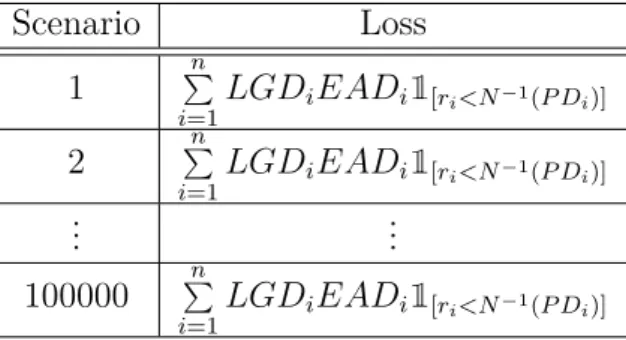
In a given scenario, the total loss of a portfolio is the sum of losses of positions in default, see (JORION, 2007) and (Pereira, 2012). To arrive at the value of the portfolio loss with 99,9% confidence level, it is necessary to simulate a big number of scenarios and take the 99,9% percentile. Our adapted IRC value will be this 99,9% percentile. See table
4for a picture.
Scenario Loss
1 Pn
i=1LGDiEADi✶[ri<N
−1(P Di)]
2 Pn
i=1LGDiEADi✶[ri<N
−1(P Di)]
... ...
100000 Pn
i=1LGDiEADi✶[ri<N
−1(P Di)]
Table 4 – Step 3 - Monte Carlo simulation of asset values to generate correlated loss.
3.4 Expected Results
Chapter 3. Model Development 33
Figure 3 – Comparison between the distribution of equity returns and credit returns.
34
4 Theory application
4.1 Description of the case study
To evaluate the impact of the adapted IRC measure, I choose forty relevant companies from the Ibovespa index. In a first evaluation, I will separate them in two portfolios of twenty stocks based on their index participation. These portfolios are described in tables 5 and 6. The idea is to evaluate portfolios with different settings. The first one, is more concentrated in some names. The second one is more equally weighted. After, i will group all stocks in a single portfolio to observe the composed effect. The weight each company will have on the portfolio will be proportional to its index weight.
Company Ticker Weight Sector
Ambev SA ABEV3 7,7% Consumer Staples Petróleo Brasileiro SA PETR4 6,1% Energy
BRF SA BRFS3 4,3% Consumer Staples
Cielo SA CIEL3 3,6% Financials
Vale SA VALE5 3,6% Materials
JBS SA JBSS3 3,1% Consumer Staples
BM&Fbovespa SA BVMF3 2,4% Financials
Embraer SA EMBR3 2,0% Industrials
Kroton Educacional SA KROT3 1,9% Consumer Discretionary Telefônica Brasil SA VIVT4 1,7% Communications
Lojas Renner SA LREN3 1,6% Consumer Discretionary Cia Brasileira de Dist. PCAR4 1,4% Consumer Staples
CCR SA CCRO3 1,4% Industrials
CEMIG CMIG4 1,1% Utilities
Cia Siderúrgica Nacional SA CSNA3 0,5% Materials Cyrela Brazil Realty SA CYRE3 0,3% Financials
Usiminas SA USIM5 0,2% Materials
PDG Realty SA PDGR3 0,0% Financials
OGX SA OGXP3 0,0% Energy
MMX SA MMXM3 0,0% Materials
Table 5 – Ibovespa index companies used in the first portfolio study.
Chapter 4. Theory application 35
Company Ticker Weight Sector
Fibria Celulose SA FIBR3 1,0% Materials Souza Cruz SA CRUZ3 1,0% Consumer Staples Suzano Papel e Celulose SA SUZB5 1,0% Materials
Tim Participações SA TIMP3 1,0% Communications Tractebel Energia SA TBLE3 1,0% Utilities
CPFL Energia SA CPFE3 1,0% Utilities
BR Malls Participações SA BRML3 1,0% Financials
Estácio Participações SA ESTC3 1,0% Consumer Discretionary Natura Cosméticos SA NATU3 1,0% Consumer Discretionary Localiza Rent a Car SA RENT3 1,0% Consumer Discretionary Cia Paranaense de Energia CPLE6 0,0% Utilities
Cia Energética de São Paulo CESP6 1,0% Utilities
Hypermarcas SA HYPE3 1,0% Health Care
Braskem SA BRKM5 1,0% Materials
EDP - Energias do Brasil SA ENBR3 0,0% Utilities
Oi SA OIBR4 0,0% Communications
Cia Hering HGTX3 0,0% Consumer Discretionary Marcopolo SA POMO4 0,0% Consumer Discretionary Gafisa SA GFSA3 0,0% Consumer Discretionary Gol Linhas Aéreas Inteligentes SA GOLL4 0,0% Consumer Discretionary
Table 6 – Ibovespa index companies used in the second portfolio study.
MMX are not present in the Ibovespa index anymore since they filed for bankruptcy.
4.2 Data selection
We use Matlab connected to an Access table, containing the stock information, for calculating the parameters in KMV Moody’s methodology. The code implemented solves, simultaneously, the two nonlinear eqs. (3.13) and (3.20) to work out the value and volatility of the firm’s assets. Afterwards, we start to solve the Distance-to-Default in eq. (3.11) and the Probability of Default eq. (3.10). The calculation steps are in the following
sequence:
4.2.1 KMV Moody’s - Parameter Estimation
• The volatility of equity
The volatility of the equity is calculated by the historical equity return data. Since in the assumption that the stock price follows the geometric Brownian motion, we would assume that µi is the log return at the ith day, Si and Si−1 are the closing
Chapter 4. Theory application 36
the log return and in eq.(4.2) we have the volatility of the equity, which will be calculated for 252 trading days.
µi = ln
Si
Si−1
(4.1)
σE = v u u
t n
n−1
n X i=1 µ2 i − 1
n−1(
n X
i=1
µi)2 (4.2)
• The market value of equity
This is calculated is the number of shares times the equity price. The number of shares was obtained from the quarterly balance sheet.
• Risk-free interest rate
In this case I used the first future of DI as the risk-free interest rate.
• Time
The company maturity was set as one year to calculate the Probability of Default.
• Liability of the Firm
Obtained from the quarterly balance sheet. In the KMV model, the liabilities are equal to the short-term plus one half of the long-term one. This is done to define the default point.
• The value an volatility of the firm’s asset
The two nonlinear eqs. (3.13) and (3.20) use as input the five parameters above. To solve this system of equations they are modified to the equations eqs. (4.3) and (4.4), as show below:
f(At) =AtN(d1)−Lexp(−rT)N(d2)−Et (4.3)
f(σE) =
N(d1)AtσA
Et −
σE (4.4)
The basic idea of the calculations are listed step by step below:
1. The initial volatility of the firm’s asset is replaced by the volatility of the equity. Substituting this new value in function (4.3) we derive the corresponding value of the firm’s asset.
Chapter 4. Theory application 37
3. If the volatility of the equity calculated in step 2 is equal to the estimated volatility of the equity, the program stops. Otherwise, we need to readjust the volatility of the firm’s asset, and iterate the step 1 and 2 till the condition in step 3 is reached. The solution of this system of equations is unique, see (LU, 2008).
• Distance-to-Default and Default Probability
Lastly, we apply the result obtained in the previous items to calculate the Distance-to-default and the default probability using eqs. (3.11) and (3.10).
4.2.2 Principal component analysis - Parameter Estimation
After obtaining the PD for each issuer, we need to simulate the asset returns for comparison. To build these returns we will use as proxy the equity returns. We will use a PCA method to describe a linear independent base, composed by the eigenvectors of the asset returns. We will use a Matlab routine to obtain the eigenvectors and eigenvalues from the asset returns.
There are as many eigenvectors as stock names, since we will use portfolios of twenty different companies, there will be twenty different eigenvectors and eigenvalues. The biggest eigenvalue is associated to the biggest variance. In our study, we will select the eigenvectors based in their proportional variance in such a way that the sum of the variance of the chosen ones, will represent more than 90% of the total variance.
In appendix B there are the result of some months to which the PCA was applied.
4.3 Application to the case
To simulate the loss of the portfolio, we follow the idea presented in the figure 1. First, we need to simulate the asset returns and compare the results with the monthly PD from all companies. We use the monthly PD for the equities case since liquidity horizon is one month. The eq. (4.5) relate the PD of one year to a monthly PD. This is based in a binomial process. Thus, the probability of not defaulting in one year is the same the composed probability of non-defaulting in twelve months in a roll.
(1−P D1month)12= 1−P D1year ⇒P D1month = 1− 12 q
1−P D1year (4.5)
Chapter 4. Theory application 38
39
5 Result Discussion
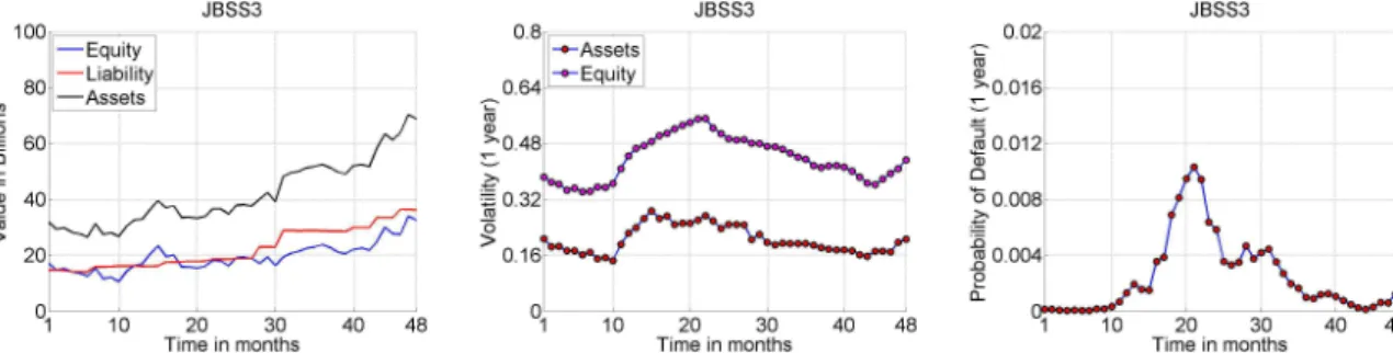
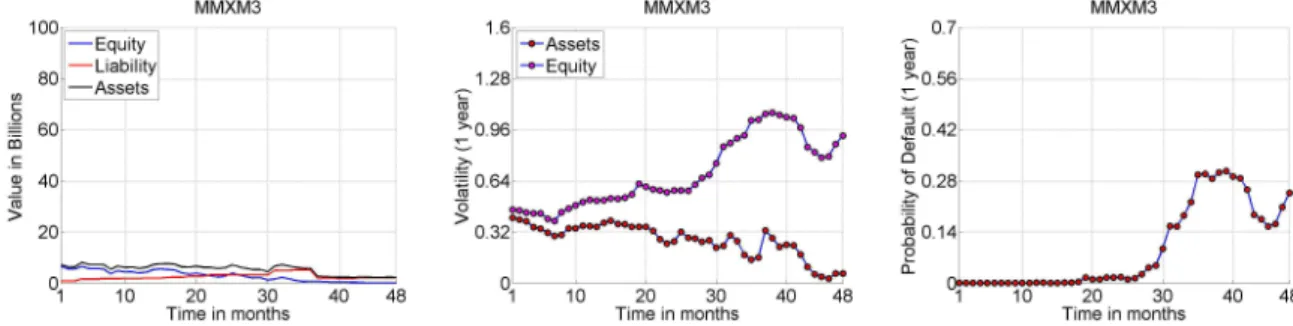
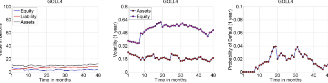
As mentioned before, the first step is to calculate the PD. First, I will present these results and after I will analyze them. The figures4to23present the asset behavior and the analysis of the credit risk of the first set of stocks. In order to compare, and understand the results, I displayed side by side the stock information and analysis, such as: first, the value of the assets, liabilities and equity; second, the volatility of the assets and equity; and third, the PD. The graphs present different scales, both in the asset values and in PD. I tried to maintain the same scale, when possible, but some information and obtained results are very different.
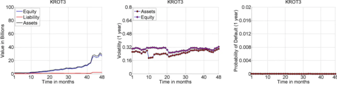
Many of these stocks present very low PD, most of the time near to zero. Such as Ambev in figure 4, BRF in figure 6, Cielo in figure 7, Vale in figure 8, BMF&Bovespa in figure 10, Embraer in figure 11, Kroton in figure 12, Vivo in figure 13, Lojas Renner in figure 14, Cia Brasileira de Distribuição in figure15, CCR in figure 16, CEMIG in figure
17. Analyzing the graphs, the results make sense, since these companies present the market value of equity above the value of liabilities, which means that in the simulation these companies did not reach the default point. This is the most prominent reason that justify the fact that the implied PD calculated was near zero.
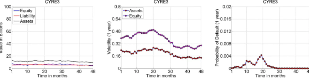
On the other hand, we may notice other two types of stocks. The first one is represented by the companies: Petrobrás in figure 5, JBS in figure 9, Cia Siderúrgica Nacional in figure 18, Cyrela in figure19, Usiminas in figure 20and PDG in figure 21. This group of stocks present a PD different of zero, but most of them lower than 2%, except for PDG which present a PD lower than 4%. All the cases present the market value of equity lower than the value of the liabilities and high volatility. In the Petrobrás, Cia Siderúrgica Nacional and PGD cases, it is very clear the effect of the value of the liabilities crossing the market value of equity, followed by an increase of volatility, this caused the value of the PD to increase. In the JBS, Cyrela, and Usiminas cases, the effect of the volatility is prominent, which may be observed in the middle of the period.
Chapter 5. Result Discussion 40
Figure 4 – ABEV3 Assets Behavior and Probability of Default
Figure 5 – PETR4 Assets Behavior and Probability of Default
Figure 6 – BRFS3 Assets Behavior and Probability of Default
Chapter 5. Result Discussion 41
Figure 8 – VALE5 Assets Behavior and Probability of Default
Figure 9 – JBSS3 Assets Behavior and Probability of Default
Figure 10 – BVMF3 Assets Behavior and Probability of Default
Chapter 5. Result Discussion 42
Figure 12 – KROT3 Assets Behavior and Probability of Default
Figure 13 – VIVT4 Assets Behavior and Probability of Default
Figure 14 – LREN3 Assets Behavior and Probability of Default
Chapter 5. Result Discussion 43
Figure 16 – CCRO3 Assets Behavior and Probability of Default
Figure 17 – CMIG4 Assets Behavior and Probability of Default
Figure 18 – CSNA3 Assets Behavior and Probability of Default
Chapter 5. Result Discussion 44
Figure 20 – USIM5 Assets Behavior and Probability of Default
Figure 21 – PDGR3 Assets Behavior and Probability of Default
Figure 22 – OGXP3 Assets Behavior and Probability of Default
Figure 23 – MMXM3 Assets Behavior and Probability of Default
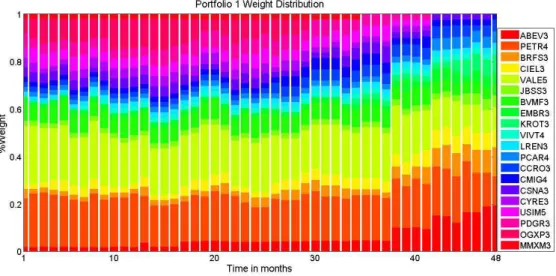
Chapter 5. Result Discussion 45
this is presented in figure 25. The weight of each share in the portfolio is proportional to the index weight.
The adapted IRC vs. VaR graph, in figure 24 increases rapidly after time 15 mainly because of JBS, Cyrela and PDG which present a considerable PD and a relevant participation in the portfolio. After, the time 25 the measure begins to spike again due to the OGX and MMX effects. But as time passes, the participation of these companies decrease, this may be observed in figure 25.
A second aspect of the figure24is the comparison with a VaR with 99% confidence level for a 252 trading days window, in annex B is a description of how to calculate the VaR. I choose the 252 days window because the IRC is a one year measure, thus they cover the same period of time. Compared to the VaR, the effect of the adapted IRC is more relevant in portfolios with issuers of higher PD. The value of VaR varies with variation of the equity volatilities and component weights.
In figure 24there also is a 10-days VaR, but with a different scale. Although this VaR with a smaller observation window is lower, when it is introduce in the capital formula, it is multiplied by some internal factor, see annex A. The final effect is the same of having a 252 days VaR, because the multiplying factor is bigger than 3.
The survey presented in the BIS document (SETTLEMENTS, 2009a) indicates that the IRC measure may increase the capital allocation in the trading book in some cases in more than 100%. This may be observed in 24, in portfolios of higher PD the importance of the IRC increases. Thus by comparing the graphs we conclude that the IRC in fact may increase the capital allocation in even 100% and that it depends a lot in the credit quality of the companies in the portfolio.
Chapter 5. Result Discussion 46
Figure 25 – Weight Distribution of Portfolio 1 over time
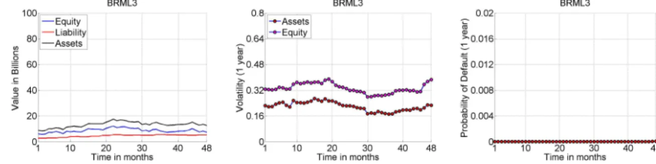
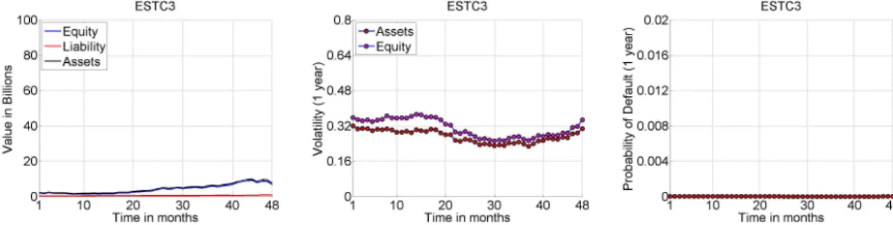
Just as in the first portfolio, in the analysis of the second will begin by calculating the PD for each issuer. The figures 26 to45 present the asset behavior and the analysis of the credit risk of the first set of stocks. One more time, in order to compare, and understand the results, I displayed side by side the stock information and analysis, such as: first, the value of the assets, liabilities and equity; second, the volatility of the assets and equity; and third, the PD. Some PD graphs present different scales.
Again many of these stocks present very low PD, most of the time near to zero. Such as BR Malls in figure 27, CPFL Energia in figure 29, Cia Paranaense de Energia in figure 30, Souza Cruz in figure31, EDP - Energias do Brasil in figure 32, Estacio in figure
33, Hering in figure 37, Natura in figure 39, Marco Polo in figure 41, Localiza in figure
42, Tractebel in figure44, Tim in figure 45. Just as in the first portfolio, analyzing the graphs of the second portfolio, the results make sense, since these companies present the market value of equity above the value of liabilities, which means that in the simulation these companies did not reach the default point. This is the reason that justify the fact that the implied PD calculated was near zero.
Chapter 5. Result Discussion 47
Figure 26 – BRKM5 Assets Behavior and Probability of Default
Figure 27 – BRML3 Assets Behavior and Probability of Default
Figure 28 – CESP6 Assets Behavior and Probability of Default
Chapter 5. Result Discussion 48
Figure 30 – CPLE6 Assets Behavior and Probability of Default
Figure 31 – CRUZ3 Assets Behavior and Probability of Default
Figure 32 – ENBR3 Assets Behavior and Probability of Default
Chapter 5. Result Discussion 49
Figure 34 – FIBR3 Assets Behavior and Probability of Default
Figure 35 – GFSA3 Assets Behavior and Probability of Default
Figure 36 – GOLL4 Assets Behavior and Probability of Default
Chapter 5. Result Discussion 50
Figure 38 – HYPE3 Assets Behavior and Probability of Default
Figure 39 – NATU3 Assets Behavior and Probability of Default
Figure 40 – OIBR4 Assets Behavior and Probability of Default
Chapter 5. Result Discussion 51
Figure 42 – RENT3 Assets Behavior and Probability of Default
Figure 43 – SUZB5 Assets Behavior and Probability of Default
Figure 44 – OGXP3 Assets Behavior and Probability of Default
Figure 45 – TIMP3 Assets Behavior and Probability of Default
Chapter 5. Result Discussion 52
stock in the first portfolio, this is presented in figure 47. The weight of each share in the portfolio is proportional to the index weight.
The adapted IRC vs. VaR graph, in figure46is very different from the first portfolio case. This happens because the issuer participation in the portfolio behaves differently. The second portfolio is more homogeneous, the participation of stocks like Gafisa, Oi and Gol is relevant during the first half of the time. As time passes, the participation of the issuers of higher PD decreases and so does the adapted IRC. The spikes in the graph occur because the index participation vary a lot for time to time interval.
As second aspect of the figure 46, we compare the adapted IRC with a VaR of 252 trading days window and 99% confidence level. This portfolio has issuers with lower volatility and this influences the VaR value. On the other hand, as we may see in the figure, the IRC may reach more than 100% of loss. This is merely consequence of its structure. This is called the constant level of risk, which simplifies the assumption to frequently rebalance or rollover the positions, at the liquidity horizon, in a manner that it maintains the initial level of risk. In other words, this happens because in a one year window, we evaluate the possibility of the default happening twelve times, the equities liquidity horizon is one month.
Again, just as a reminder, in figure 46 there also is a 10-days VaR. Because, this is the VaR used in the capital formula, but it enters the formula multiplied by some internal factor, see annex A. The final effect is the same of having a 252 days VaR, because the multiplying factor is bigger than 3.
Figure 46 – Adapted IRC vs. VaR comparison for Portfolio 2
For the last analysis, we use a third portfolio, which is more diluted in terms of stock participation. This is exhibited in figure 48. In this last, case, as we may have anticipated the more relevant shape derives from the first portfolio, which was the one with larger weights.
Chapter 5. Result Discussion 53
Figure 47 – Weight Distribution of Portfolio 2 over time
VaR. As, we may also notice, in portfolios more diversified the IRC decreases, because the stocks with more relevance in the portfolio have lower probability of default. But, nonetheless it still is relevant when compared to the VaR and the results still indicates a possible high increase in capital allocation, if the measure is used in the allocation formula.
One last remark should be made, that is the fact that the measure was able to predict and anticipate default events of some names in the portfolio. This is something a VaR is not capable to do, independent of the trading days window considered. This means that the increase in PD of some relevant companies in the portfolio influenced the value of the adapted IRC to increase as well.
54
6 Conclusion
In this dissertation, we addressed an issue of evaluating the effect of default for capital allocation in the trading book, in the case of public equities. And more specifically, in the Brazilian Market. This problem emerged because of recent crisis, which increased the need for regulators to impose more allocation in banking operations. This is especially valid for the trading book. For this reason, the BIS committee, recently introduce a new measure of risk, the Incremental Risk Charge.
This measure of risk, is basically a one year value-at-risk, with a 99.9% confidence level. The IRC intends to measure the effects of credit rating migrations and default, which may occur with instruments in the trading book. This measure is mainly used for credit products. For this reason, the past works about this subject only referenced portfolio of bonds. Even, the Basel Committee does not impose certain products to be modeled for this measure, such is equities. Although, as we saw, some banks, model the measure for equities.
The main reason for not performing such modelling, is the fact that there is not a clear relation of credit rating migrations and equity returns. Some references indicate a clear relation for downgrades, but they also demonstrate the that this relation is not clear for upgrades. For this reason, we choose a simpler path to address this problem. We adapted the IRC, by ignoring the need to evaluate the credit rating migrations. As a matter of fact, we only considered the effect of the default for computing the measure.
Since we choose to follow this path, the more adequate choice of model, to evaluate credit risk was the KMV model, which is an structural model, based in the Merton model. This model was used to calculate the PD for the issuers used as case tests. Even, in this model I had to assume certain simplicities, such as the normal distribution for calculating the PD and we only calculated implied PD’s, since we did not have information about the assets growth. These are all practical approaches that permit to simplify the problem on order to solve it.
After, calculating the issuer’s PD, I simulated the returns with a Monte Carlo after using a Principal Analysis Decomposition. This approach permitted to obtain a practical way the correlated returns for simulating the portfolio loss. In our case, since we are dealing with stocks, the LGD was supposed as constant and with value determined by a BIS document.
Chapter 6. Conclusion 55
VaR, with a 99% confidence level. The comparison with a 252-days VaR is more adequate since the IRC is a one year measure, although the 10-day VaR has different weight in the capital allocation formula, which makes it almost as the same effect of the 252-days VaR.
The portfolios used in the calculations were composed by listed stocks of the Ibovespa index. We compared different types of portfolios, so we could be able to understand different effects present in each of them. The first portfolio had stocks with higher PD and cases that defaulted. The second one, was a more concentrated portfolio, and the adapted IRC varied a lot with the weight change of each stock. The third one, was a composition of the first and the second. This permitted to confirm the more prominent participation of the first portfolio in dictating the behavior of the measure. Besides that, we observed that increases in portfolio volatility increased the VaR measure, and increased the IRC as well. But, the most important to the IRC is the increase in PD, which increases with the volatility, but mainly increase with the Debt to Equity relation increase.
One last and important remark is that Banks generally have lower expositions to equity in their portfolio. In light of this, one might say that this risk measure would not make a big difference, but there are several Hegde Funds that are highly exposed to equity risk that could use this risk measure.