Annales
Geophysicae
Estimating the contribution from different ionospheric regions to
the TEC response to the solar flares using data from the
international GPS network
L. A. Leonovich, E. L. Afraimovich, E. B. Romanova, and A. V. Taschilin
Institute of Solar-Terrestrial Physics SD RAS, Irkutsk, Russia
Received: 21 February 2002 – Revised: 27 May 2002 – Accepted: 20 June 2002
Abstract. This paper proposes a new method for estimat-ing the contribution from different ionospheric regions to the response of total electron content variations to the solar flare, based on data from the international network of two-frequency multichannel receivers of the navigation GPS sys-tem. The method uses the effect of partial “shadowing” of the atmosphere by the terrestrial globe. The study of the solar flare influence on the atmosphere uses GPS stations located near the boundary of the shadow on the ground in the nightside hemisphere. The beams between the satellite-borne transmitter and the receiver on the ground for these stations pass partially through the atmosphere lying in the region of total shadow, and partially through the illuminated atmosphere. The analysis of the ionospheric effect of a pow-erful solar flare of class X5.7/3B that was recorded on 14 July 2000 (10:24 UT, N 22 W 07) in quiet geomagnetic con-ditions (Dst = −10 nT) has shown that about 75% of the
TEC increase corresponds to the ionospheric region lying be-low 300 km and about 25% to regions lying above 300 km. Key words. Ionosphere (solar radiation and cosmic ray ef-fects; instruments and techniques) – Solar physics, astro-physics and astronomy (ultraviolet emissions)
1 Introduction
The enhancement of X-ray and ultraviolet (UV) emission that is observed during chromospheric flares on the Sun im-mediately causes an increase in electron density in the iono-sphere. These density variations are different for different altitudes and are called Sudden Ionospheric Disturbances (SIDs) (Davies, 1990; Donnelly, 1969). SIDs are gener-ally recorded as the short wave fadeout (SWF) (Stonehocker, 1970), sudden phase anomaly (SPA) (Ohshio, 1971), sud-den frequency deviation (SFD) (Donnelly, 1971; Liu et al., 1996), sudden cosmic noise absorption (SCNA) (Deshpande and Mitra, 1972), and sudden enhancement/decrease of at-Correspondence to:E. L. Afraimovich ([email protected])
mospherics (SES) (Sao et al., 1970). Much research is de-voted to SID studies, among them a number of thorough re-views (Mitra, 1974; Davies, 1990).
A highly informative technique is the method of Inco-herent Scatter (IS). The Millstone Hill IS facility recorded a powerful flare on 7 August 1972 (Mendillo and Evans, 1974a). The measurements were made in the height range from 125 to 1200 km. The increase in local electron density Nemade up 100% at 125 km altitude and 60% at 200 km.
Using the IS method, Thome and Wagner (1971) obtained important evidence of the height distribution of the increase inNe at the time of the 21 and 23 May 1967 flares. A
sig-nificant increase inNe was recorded in the E-region, up to
200%, which gradually decreased in the F-region with in-creasing height, down to 10–30%, and remained distinguish-able up to 300 km. The earliest increase inNe began in the
E-region, and at higher altitudes it was observed with a delay which is particularly pronounced at F-region heights.
A sudden increase in total electron content (TEC) can be measured using continuously operating radio beacons installed on geostationary satellites. On 7 August 1972, Mendillo et al. (1974b) were the first to make an attempt to carry out global observations of the solar flare using 17 stations in North America, Europe, and Africa. The obser-vations covered an area, the boundaries of which were sep-arated by 70◦in latitude and by 10 h in local time. For
dif-ferent stations, the absolute value of the TEC increase1I varies from 1.8·1016to 8.6·1016el·m−2, which corresponds to 15–30% of the TEC. Investigations revealed a latitudinal dependence of the TEC increase value. At low latitudes, it was higher compared with high latitudes. Besides, the au-thors point out the absence of a connection between the TEC increase value and the solar zenith angle.
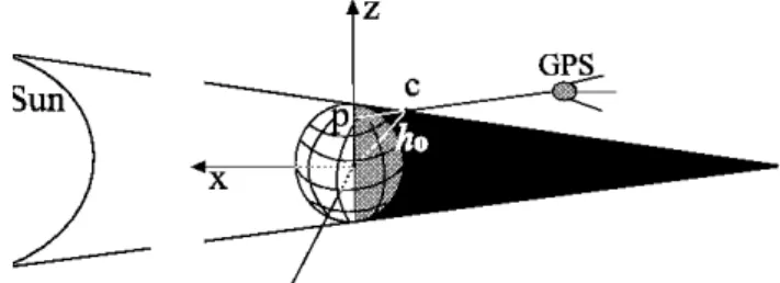
Fig. 1.Scheme for the determination of the shadow altitudeh0over the ground in the GSE system. GPS – GPS navigation satellite; P – GPS station on the ground; C – intersection point of the transmitter – receiver LOS and the shadow boundary.
receiver on the ground and transmitters on the GPS system satellites covering the reception zone are made using two-frequency multichannel receivers of the GPS system at al-most any point of the globe and at any time, simultaneously at two coherently coupled frequencies: f1 =1575.42 MHz andf2=1227.60 MHz.
The sensitivity of phase measurements in the GPS system is sufficient for detecting irregularities with an amplitude of up to 10−3−10−4of the diurnal TEC variation. This makes it possible to formulate the problem of detecting ionospheric disturbances from different sources of artificial and natural origins. The TEC unit (TECU), which is equal to 1016el· m−2and is commonly accepted in the literature, will be used throughout the text.
Afraimovich (2000a) and Afraimovich et al. (2000b, 2001a, b) have developed a novel technology of a global de-tection of ionospheric effects from solar flares and presented data from first the GPS measurements of global response of the ionosphere to powerful impulsive flares of 29 July 1999 and 28 December 1999. The authors found that fluctuations of TEC are coherent for all stations on the dayside of the Earth. The time profile of TEC responses is similar to the time behavior of hard X-ray emission variations during flares in the energy range 25–35 keV if the relaxation time of elec-tron density disturbances in the ionosphere of the order of 50–100 s is introduced. No such effect on the nightside of the Earth has been detected yet.
Afraimovich et al. (2001c, 2002) and Leonovich et al. (2001) have suggested a technique for estimating the iono-spheric response to weak solar flares (of X-ray class C). They obtained a dependence of the ionospheric TEC increase am-plitude (during the solar flare) on the flare location on the Sun (on the central meridian distance, CMD). For flares ly-ing closer to the disk center (CMD<40◦), an empirical
de-pendence of the ionospheric TEC increase amplitude on the peak power of solar flares in the X-ray range was obtained (using data from the geostationary GOES-10 satellite).
This paper is a logical continuation of the series of our publications (Afraimovich, 2000a; Afraimovich et al., 2000b, 2001a, b, c, 2002; Leonovich et al., 2001) devoted to the study of ionospheric effects of solar flares, based on data from the international GPS network.
A limitation of the GPS method is that its results have an integral character. It is therefore impossible to determine (from measurement at a single site) the particular ionospheric region which makes the main contribution to the TEC varia-tion. The objective of this study is to develop a method which would help overcome (at least partially) this problem.
2 Method of determining the shadow altitude h0 over the ground
The method uses the effect of partial “shadowing” of the atmosphere by the terrestrial globe. Direct beams of solar ionizing radiation from the flare do not penetrate the region of the Earth’s total shadow. GPS stations located near the shadow boundary on the ground in the nightside hemisphere are used to investigate the solar flare influence on the iono-sphere. The LOS for these stations pass partially through the atmosphere lying in the total shadow region, and partially through the illuminated atmosphere. The altitude over the ground at which the LOS intersects the boundary of the total shadow cone will be referred to as the shadow altitudeh0.
Figure 1 schematically represents the formation of the cone of the Earth’s total shadow (not to scale) in the geo-centric solar-ecliptic coordinate system (GSE): the axisZis directed to a north perpendicular planes of an ecliptic, and the axisX– on the Sun, and the axisY is directed perpen-dicular to these axes. For a definition of the shadow altitude h0, it is necessary to know the coordinates of a cross point C of the LOS and the shadow boundary.
The primary data are the geographical coordinates of sta-tion GPS on the Earth (Fig. 1; a point P): an elevasta-tion angle θ and azimuth of LOS on a satellite GPS, toward the north clockwise, for the time (UT), corresponding to the phase of solar flare maximum in the X-ray range. These coordinates are converted to the Cartesian coordinate system, where the Cartesian coordinates of the GPS station on the ground and the coordinates of the subionospheric point (at 300 km al-titude) are calculated. Next, we use the geocentric solar-ecliptic coordinate system following the technique reported by Sergeev and Tsyganenko (1980). To determine the coor-dinates of the point C, we solve a system of equations: the equation of a cone (of total shadow), and the equation of a straight line (LOS) specified parametrically. After that, from the resulting point C, we drop a perpendicular to the ground and calculate its length (Fig. 1, lineh0). Thus, the obtained value ofh0is just the shadow altitude.
3 Method of determining the TEC increase in the iono-sphere using data from the global GPS network
This paper exemplifies an analysis of the ionospheric effect of a powerful solar flare of class X5.7/3B recorded on 14 July 2000 (10:24 UT, N 22 W 07) under quiet geomagnetic conditions (Dst = −10 nT). The time profile of soft X-ray
/((3K
R
NP
0
2
4
L(
t)
9 .6
1 0
1 0 .4 1 0 .8 1 1 .2
T im e , U T
0
0 .2
0 .4
∆
I(
t)
, TECU
)
,
W
m
-2
.
10
3
a
b
d
e
*2(6
0
2
4
I(
t)
, T
E
C
U
0
2
4
I'
(t),
T
E
C
U
c
9
9
A (t)
C (t)
B (t)
C (t)
D (t)
∆
I
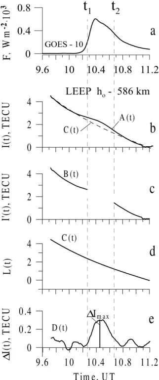
m a xFig. 2. Time profile of soft X-ray emission in the range 1–
8 ˚A(GOES-10 data) during the solar flare of 14 July 2000(a). Time dependence of TEC variations for the station LEEP A(t) (PRN07, shadow height ho = 586 km)(b), solid line. The same dependence after removal of counts in interval (t1−t2)(c)is represented by curve B(t).(d)is the curve C(t) (third-degree polynomial) approx-imating the time dependence B(t). This same curve is plotted in panel (b) by a dashed line. Time dependence of TEC variations D(t) upon subtracting the polinom(e).
To determine the TEC increase in the ionosphere we used the data from the international GPS network. The GPS
tech-nology provides a means of estimating the TEC variations I0(t )on the basis of TEC phase measurements made with each of the spatially separated two-frequency GPS receivers using the formula (Calais and Minster, 1996):
I0(t )= 1 40.308
f12f22
f12−f22[(L1λ1−L2λ2)+const+nL],(1) whereL1λ1andL2λ2are the increments of the radio signal phase path caused by the phase delay in the ionosphere (m); L1andL2stand for the number of complete phase rotations, andλ1 andλ2are the wavelengths (m) for the frequencies f1andf2, respectively; const is some unknown initial phase path (m); andnLis the error in determining the phase path (m).
Input data used in the analysis include a series of the “oblique” values of TECI0(t ), as well as a corresponding series of elevationsθ and azimuths of LOS to the satellite. These parameters are calculated using our developed CON-VTEC program to convert standard (for the GPS system) RINEX-files received via the Internet. Input series of TEC I0(t )are converted to the “vertical” value following a well-known technique (Klobuchar, 1986):
I (t )=I0·cos
arcsin
R
E
RE+hmax cosθ
, (2)
where RE is Earth’s radius; and hmax is the height of the ionosphericF2-layer maximum.
Variations of the regular ionosphere, as well as trends in-troduced by the motion of the satellite, are eliminated us-ing the procedure of removus-ing the trend. The procedure of eliminating the trend for each realization is presented in Fig. 2. The time profile of soft X-ray emission in the range 1–8 ˚A(GOES-10 data) during the solar flare of 14 July 2000 is shown in Fig. 2a. Figure 2b (solid line) presents the typ-ical time dependence of verttyp-ical TEC A(t) for the site GPS LEEP (PRN07, shadow heighth0= 586 km). From this de-pendence we eliminated the counts corresponding to inter-val (t1 −t2), during which (according to GOES-10 data) soft X-ray emission showed the phase of flare maximum (from 10:18 to 10:35 UT) – Fig. 2b, curveB(t ). The depen-denceB(t ), obtained by this procedure, was approximated by a third-order polynomialC(t )using the least-squares tech-nique. The polynomialC(t )is shown in Figs. 2d and c by a dashed line. The resulting TEC responseD(t )is deduced as a difference: D(t ) =A(t )−C(t ), Fig. 2e. A maximum value of the response1Imax, shown in Fig. 2e by a vertical line, is then used to estimate the contribution from different ionospheric regions to the TEC response.
4 Results and discussion
Table 1.Parameters of response TEC during solar flare of 14 July 2000
Site PRN h0 1Imax M latitude longitude
GPS km TECU % degree degree
STB1 2 0 1.1 100 44.7 272
KAYT 21 0 1.06 96.3 13.9 120
STL4 2 15 1.1 100 38.6 270
WDLM 2 16 1.07 97.2 44.6 264
SLAI 2 21 1.09 99.0 41.9 266
GUS2 2 65 1.0 90 58.3 225
PRDS 9 80 1.1 100 50.8 245
CORD 1 92 1.0 90.9 −31.5 295
WILL 2 107 0.9 81.8 52.2 237
YAR1 17 112 1.0 90.9 −29.0 115
PLTC 2 140 0.83 75.4 40.1 255
VCIO 7 141 0.8 72.7 36.0 260
TMGO 2 147 0.72 65.4 40.1 254
PATT 7 147 0.71 64.5 31.7 264
DSRC 2 150 0.7 63.6 39.9 254
LKWY 9 152 0.71 64.5 44.5 249
PERT 30 155 0.66 60 −31.8 115
NANO 2 175 0.54 49.0 49.2 235
WHD1 2 185 0.5 45.4 48.3 237
SEAW 2 194 0.41 37.2 47.6 237
UCLU 2 195 0.5 45.4 48.9 234
SEAT 2 195 0.49 44.5 47.6 237
LIND 9 205 0.46 41.8 47 239
SEAW 9 206 0.42 38.1 47.6 237
GOBS 2 221 0.44 40 45.8 239
SATS 2 222 0.34 30.9 46.9 236
GWEN 2 227 0.32 29.0 45.7 238
LMUT 2 233 0.4 36.3 40.2 248
LKHU 4 234 0.39 35.4 29.9 264
AZCN 7 280 0.35 31.8 36.8 252
FTS1 7 280 0.3 27.2 46.2 236
SHIN 2 339 0.29 26.3 40.5 239
TUNG 9 344 0.28 25.4 40 241
SMYC 9 412 0.3 27.2 36.3 244
JAB1 17 413 0.3 27.2 −12.6 132
UCLP 2 483 0.31 28.1 34.0 241
CVHS 9 520 0.27 24.5 34.0 242
LEEP 7 585 0.28 25.4 34.1 241
PMHS 7 590 0.25 22.7 33.9 241
UCLP 7 590 0.26 23.6 34.0 241
CSDH 7 594 0.25 22.7 33.8 241
YBHB 26 685 0.24 21.8 41.7 237
RIOG 13 704 0.25 22.7 −53.7 292
PTSG 26 719 0.26 23.6 41.7 235
GUAM 26 885 0.23 20.9 15.5 154
which the signal is received (PRN), shadow altitude above
the ground (h0), absolute increase in TEC1Imax, relative
increase of TECM =1 Imax/1 I0, and geographical
coor-dinates of GPS stations (latitude, longitude). The increase of
TEC1I0corresponds to the amplitude of the TEC increase
measured at the station lying at the shadow boundary on the
ground (h0=0).
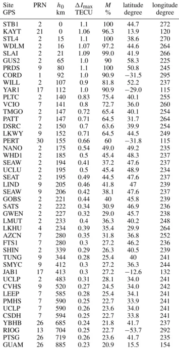
Figure 3b illustrates examples of time dependencies of the TEC1I (t ) response for LOS to the satellites which inter-sect the boundary of the shadow cone at different heights
h0 during the solar flare of 14 July 2000. Figure 3b (left)
presents the values of these altitudes, and (right) the names of the corresponding stations. For a better visualization, the
35'6 :,// <$5 3(57 /((3
&9+6
8&/3
376*
&6'+
6+,1
1$12 /,1' 60<&
$=&1
:'/0
9.2 9.6 10 10.4 10.8 11.2 11.6
T IM E , U T
67%
TE
C
U
_
_
T IM E , U T
)
, W
m
-2.10
3
*2(6
KRNP ∆I(t), T E C U 6WDWLRQV
*8$0
a
b
Fig. 3. Time profile of soft X-ray emission in the range 1–
8 ˚A(GOES 10 data)(a). Examples of time dependencies of the TEC response1I (t )for LOS intersecting the boundary of the shadow cone at different altitudesh0during the solar flare of 14 July 2000 (for a better visualization, the dependencies are drawn by lines of different thicknesses); the column at the left shows the values of these heights, and the column at the right shows the names of the corresponding stations(b).
U T ∆ I( t), T E C U ∆ I( t) , T E C U ∆ I( t) , T E C U
,
/
.
Sd , T E C U 10 3s -1 S d , TEC U 10 3s -1 U T Sd , T E C U 10 3s -1-
0
1
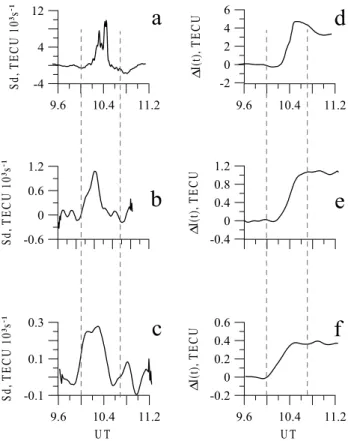
Fig. 4. Comparison of the TEC response for different conditions
of atmospheric illumination. The result of a coherent accumulation of the TEC time derivativesSdex (a), and the mean integral TEC
increment1I (t )(d)for stations located in the Earth’s illuminated hemisphere. Similar results for stations lying along the terminator line(b),(e), and for LOS crossing the shadow boundary at altitudes higher above 300 km(c),(f). Dashed lines correspond to the start and end times of the soft X-ray flare (GOES-10, 1–8 ˚A).
the shadow altitude exceeds significantly the electron density peak height in the ionosphere. For station GUAM (PRN26, height of the shadow boundaryh0 =885 km), the response amplitude exceeds the background oscillation amplitude by more than a factor of 2.
It is evident from Fig. 3 that the wave phase (time of the response maximum) is different at different altitudesh0. On the one hand, this phenomenon can be caused by the inter-ference of the response with background fluctuations; on the other, this can be due to the fact that at different heights dif-ferent wavelengths of ionizing radiation are observed, which, in turn, can have independent time characteristics.
By virtue of the fact that the response amplitude at high altitudes was found to be comparable with the level of back-ground fluctuations, the method of coherent accumulation by Afraimovich (2000a) and Afraimovich et al. (2000b, 2001a, b, c) was used in an additional analysis. The essence of the method is that it involves a coherent summation of TEC responses to the solar flare, which are measured simul-taneously with all LOS chosen for the analysis. The analysis used spatially distributed stations to provide a statistical
∆Ι
PD[
, T E C U
K
R
NP
∆Ι
PD[
/∆Ι
ο, %
Fig. 5. Dependence of the absolute TEC increase1Imaxon the
shadow altitudeh0 during the solar flare of 14 July 2000. The dashed line on the plot corresponds to the root-mean-square de-viation of background oscillations in the absence of a flare. The upper scale shows the dependence of the relative TEC increase
1Imax/1I0on the shadow altitudeh0during the solar flare in
per-cent. The TEC increase1I0corresponds to the amplitude of the TEC increase measured at the station lying on the shadow bound-ary on the groundh0=0.
dependence of background fluctuations for spaced LOS. As-suming that the TEC response to the solar flare is the signal and the background TEC fluctuations are noise, it is found that because the background fluctuations are not correlated at spaced LOS, the signal-to-noise ratio increases through a coherent processing no less than by a factor of√N, where Nis the number of the LOS used.
In the present case, the coherent summation of the time derivatives was used for all dependencies of the “vertical” TEC value under investigation. The time derivative was used because it permits us to do away with the constant compo-nent in TEC variations; furthermore, it reflects the rate of electron density variation proportional to the flux of ionizing radiation. After that, the trend was removed from the aver-aged sum of the time derivatives using the procedure outlined above. This was followed by an integration of the calculated time dependence,Sdex, to give the mean integral TEC
incre-ment on a given time interval.
presents the averaged results on a coherent accumulation of
the TEC time derivatives,Sdex, and the corresponding
inte-gral TEC increments1 I (t )for stations located in the Earth’s
illuminated hemisphere (a, d), for stations lying along the ter-minator line (b, c), and for LOS crossing the shadow bound-ary at altitudes above 300 km (c, f). For the conditions of full illumination, the terminator conditions and shadowing con-ditions, averaging was done over 50, 15 and 16 LOS, respec-tively.
The analysis reveals that the mean amplitude of the TEC response in the daytime hemisphere is larger by a factor of 4 than the response along the terminator line. In spite of the fact that the mean response amplitude along the LOS cross-ing the shadow boundary at altitudes above 300 km is nearly smaller by a factor of 3 than that along the terminator line, the response was sufficiently well pronounced. The coherent accumulation result confirms the presence of the response at altitudes above 300 km.
The dependence of the absolute TEC increase (1Imax) on the altitudeh0for all the cases under consideration is plotted in Fig. 5. The upper scale shows the dependence of the rela-tive TEC increaseM=1 Imax/1 I0on the shadow altitude h0during the solar flare in percent. The TEC increase1I0 corresponds to the amplitude of the TEC increase measured at the station lying on the shadow boundary on the ground h0=0.
Figure 5 suggests that about 75% of the TEC increase cor-responds to the ionospheric region lying below 300 km and about 25% to regions lying above 300 km. We found that a rather significant contribution to the TEC increase is made by ionospheric regions lying above 300 km.
The estimate obtained is consistent with the findings re-ported by Mendillo and Evans (1974a); Mendillo et al. (1974b). The authors of the cited references, based on in-vestigating the electron density profile in the height range from 125 km to 1200 km using the IS method, concluded that about 40% of the TEC increase during the powerful flare on 7 August 1972 corresponds to ionospheric regions lying above 300 km. However, Thome and Wagner (1971), who used the IS method to investigate the ionospheric effects from two others powerful solar flares, pointed out that an increase in electron density associated with the solar flare was observ-able to 300 km altitude only. This difference can be explained by the fact that each particular solar flare is a unique event which is characterized by its own spectrum and dynamics in the flare process.
Acknowledgements. We are grateful to A. T. Altyntsev for his in-terest in this study, helpful advice and active participation in discus-sions. Authors are grateful to E. A. Kosogorov and O. S. Lesuta for preparing the input data. Thanks are also due to V. G. Mikhalkosky for his assistance in preparing the English version of the manuscript. Finally, the authors wish to thank the referees for valuable sugges-tions which greatly improved the presentation of this paper. This work was done with support from both the Russian foundation for Basic Research (grants 00-05-72026 and 01-05-65374) and RFBR grant of leading scientific schools of the Russian Federation No. 00-15-98509.
Topical Editor M. Lester thanks two referees for their help in evaluating this paper.
References
Afraimovich, E. L.: GPS global detection of the ionospheric re-sponse to solar flares, Radio Sci., 35, 1417–1424, 2000a. Afraimovich, E. L., Kosogorov, E. A., and Leonovich, L. A.: The
use of the international GPS network as the global detector (GLOBDET) simultaneously observing sudden ionospheric dis-turbances, Earth Planet. Space, 52, 1077–1082, 2000b.
Afraimovich, E. L., Altyntsev, A. T., Kosogorov, E. A., Larina, N. S., and Leonovich, L. A.: Detecting of the ionospheric effects of the solar flares as deduced from global GPS network data, Ge-omagnetism and Aeronomy, 41, 208–214, 2001a.
Afraimovich, E. L., Altyntsev, A. T., Kosogorov, E. A., Larina, N. S., and Leonovich, L. A.: Ionospheric effects of the solar flares of 23 September 1998 and 29 July 1999 as deduced from global GPS network data, J. Atm. Solar-Terr. Phys., 63, 1841– 1849, 2001b.
Afraimovich, E. L., Altyntsev, A. T., Grechnev, V. V., and Leonovich, L. A.: Ionospheric effects of the solar flares as de-duced from global GPS network data, Adv. Space Res., 27, 1333–1338, 2001c.
Afraimovich, E. L., Altyntsev, A. T., Grechnev, V. V., and Leonovich, L. A.: The response of the ionosphere to faint and bright solar flares as deduced from global GPS network data, An-nals of Geophysics, 45, 31–40, 2002.
Calais, E. and Minster, J. B.: GPS detection of ionospheric pertur-bations following a Space Shuttle ascent, Geophys. Res. Lett., 23, 1897–1900, 1996.
Davies, K.: Ionospheric radio, Peter Peregrinus, London, 1990. Deshpande, S. D. and Mitra, A. P.: Ionospheric effects of solar
flares, IV, electron density profiles deduced from measurements of SCNA’s and VLF phase and amplitude, J. Atmos. Terr. Phys., 34, 255–259, 1972.
Donnelly, R. F.: Contribution of X-ray and EUV bursts of so-lar fso-lares to Sudden frequency deviations, J. Geophys. Res., 74, 1873–1877, 1969.
Donnelly, R. F.: Extreme ultraviolet flashes of solar flares observed via sudden frequency deviations: experimental results, Solar Phys., 20, 188–203, 1971.
Klobuchar, J. A.: Ionospheric time-delay algorithm for single-frequency GPS users, IEEE Transactions on Aerospace and Elec-tronics System, AES, 23, 3, 325–331, 1986.
Leonovich, L. A., Altynsev, A. T., Afraimovich, E. L., and Grechnev, V. V.: Ionospheric effects of the solar flares as de-duced from global GPS network data. LANL e-print archive, http://arXiv.org/abs/physics/011006, 2001.
Liu, J. Y., Chiu, C. S., and Lin, C. H.: The solar flare radiation re-sponsible for sudden frequency deviation and geomagnetic fluc-tuation, J. Geophys. Res., 101, 10 855–10 862, 1996.
Mendillo, M. and Evans, J. V.: Incoherent scatter observations of the ionospheric response to a large solar flare, Radio Sci., 9, 197– 203, 1974a.
Mitra, A. P.: Ionospheric effects of solar flares, D. Reidel, Norwell, Mass., 1974.
Ohshio, M.: Negative sudden phase anomaly, Nature, 229, 239– 244, 1971.
Sao, K., Yamashita, M., Tanahashi, S., Jindoh, H., and Ohta, K.: Sudden enhancements (SEA) and decreases (DSA) of atmo-spherics, J. Atmos. Terr. Phys., 32, 1567–1573, 1970.
Sergeev, V. A. and Tsyganenko, N. A.: The Earth’s magnetosphere.
Results of researches on the international geophysical projects, “Nauka”, Moscow, (in Russian), 1980.
Stonehocker, G. H.: Advanced telecommunication forecasting tech-nique in AGY, 5th., Ionospheric forecasting, AGARD Conf. Proc., 29, 27–31, 1970.