ISSN 1549-3644
© 2010 Science Publications
Corresponding Author: Muhammad Fauzi bin Embong, Department of Computer Science and Mathematics,
University Technology MARA, Kuala Terengganu Campus, 21080 Kuala Terengganu, Malaysia
An Alternative Scaling Factor In Broyden’s Class
Methods for Unconstrained Optimization
1Muhammad Fauzi bin Embong, 2Mustafa bin Mamat, 1Mohd Rivaie and 2Ismail bin Mohd 1Department of Computer Science and Mathematics, University Technology MARA,
Kuala Terengganu Campus, 21080 Kuala Terengganu, Malaysia 2Department of Mathematics, Faculty of Science and Technology,
University Malaysia Terengganu, 21030 Kuala Terengganu, Malaysia
Abstract: Problem statement: In order to calculate step size, a suitable line search method can be employed. As the step size usually not exact, the error is unavoidable, thus radically affect quasi-Newton method by as little as 0.1 percent of the step size error. Approach: A suitable scaling factor has to be introduced to overcome this inferiority. Self-scaling Variable Metric algorithms (SSVM’s) are commonly used method, where a parameter is introduced, altering Broyden’s single parameter class of approximations to the inverse Hesssian to a double parameter class. This study proposes an alternative scaling factor for the algorithms. Results: The alternative scaling factor had been tried on several commonly test functions and the numerical results shows that the new scaled algorithm shows significant improvement over the standard Broyden’s class methods. Conclusion: The new algorithm performance is comparable to the algorithm with initial scaling on inverse Hessian approximation by step size. An improvement over unscaled BFGS is achieved, as for most of the cases, the number of iterations are reduced.
Key words: Broyden’s class, eigenvalues, Hessian, scaling factor, self-scaling variable matrices INTRODUCTION
The quasi-Newton methods are very popular and efficient methods for solving unconstrained optimization problem:
n min f (x)
x∈R (1)
where, f: Rn →R is a twice continuously differentiable function. There are a large number of quasi-Newton methods but the Broyden’s class of update is more popular. As other quasi-Newton method, the Broyden’s method are iterative, whereby at (k+1)-th iteration:
k 1 k k k
x + =x + αd (2)
where, dk denotes the search direction and αk is its step
size. The search direction, dk, is calculated by using:
k k k H g
d =− (3)
Where:
gk = The gradient of f evaluated at the current iterate
xk
k
H = The inverse Hessian approximation.
The step size αk is a positive step length chosen by
a line search so that at each iteration either:
T k k
k k k k 1 k T
k k g d f (x d ) f (x )
s y
+ α ≤ − η α (4)
Or:
T
k k k k 2 k k
f (x + αd )≤f (x )− ηg d (5)
where, η1 and η2 are positive constants.
Note that the conditions (4) and (5) are assumes in Byrd and Nocedal (1989). They cover a large class of line search strategies under suitable conditions. If the gradient of f is Lipschitz continuous, then for several well known line search satisfy the Wolfe conditions:
T
k k k k 1 k k
f (x + αd )≤f (x )− δ αd g (6)
T T
k k k k 2 k k
(g(x + αd ) d ≥ δd g (7)
where, 1 2
1
1 and 1
2
Byrd and Nocedal (1989) prove that if the ratio between successive trial values of α is bounded away from zero, the new iteration produced by a backtracking line search satisfies (4) and (5). The inverse Hessian approximation is then updated by:
T T
T k k k k k k
k 1 k T T k k
k k k k k
s s H y y h
H H v v
s y y h y
φ
+ = + − φ (8)
Where:
k k 1 k
s =x + −x (9)
k k 1 k
y =g+ −g (10)
(
)
1T 2 k k k
k k k k T T
k k k k k
s H y
v y H y
s y y H y
= −
(11)
and φ is a parameter that may take any real value. According to Dennis and More (1977), there are two updated formulae that are contained in the Broyden’s class method, namely BFGS update if the parameter φk = 0 and DFP update if φk = 1.
Consequently, (1.8) may be written as: DEP BFGS
Hφ= − φ(1 )H + φH (12) If we let φ1∈[0,1] (1.8) is called Broyden convex
family. Meanwhile, if φ1∈[0,1-σ] for σ∈[0,1] then
(1.8) is called the restricted Broyden’s class method (Byrd et al., 1987).
MATERIALS AND METHODS
Scaling the Broyden’s class method:
Self-scaling Variable Metric (SSVM) method: Many modifications have been applied on quasi-Newton methods in attempt to improve its efficiency. Now, the discussion will be on the self-scaling variable metric algorithms developed by Oren (1973) and Oren and Luenberger (1974). Multiplying Hk by γk and then
replacing γk Hk in (8), the Broyden’s class formula can
be written as:
T T
T
k k k k k k
k 1 k T k k k T
k k k k k
H y y H y y
H H v v
y H y y s
φ +
= − + φ γ +
(13)
where γk is a self-scaling parameter. The formula (13) is
known as self-scaling variable metric (SSVM) formula.
Clearly, when γk = 1, the formula (13) is reduced to
Broyden’s class update (8).
Choices of the scaling factor: The choice of a suitable scaling factor can be determined by the following theorem.
Theorem (Oren and Luenberger, 1974)
Let φ∈[0,1] and γk>0 Let Hk be the inverse
Hessian approximation and Hk 1
φ
+ be defined by (13).
Let λ1≥λ2≥…≥λn and 1 2 .... n
φ φ φ
µ ≥ µ ≥ ≥ µ be eigenvalues of Hk and Hk+1 respectively. Then the following statements
hold:
• If γ λ ≥k n 1, then n 1
φ
µ = and 1 k i 1 n k i
φ +
≤ γ λ ≤ µ ≤ γ λ i = 1,2,…,n-1
• If γ λ ≤k i 1 then n 1
φ
µ = and k i i k i 1 1
φ −
γ λ ≤ µ ≤ γ λ ≤ , i = 2,3,…,n
• If γ λ ≤ ≤ γ λk 1 1 k 1 and i0 is an index with
k i0 1 k i0
γ λ ≤ ≤ γ λ k 1 1 k 2 1 2 ... k i0
φ φ
γ λ ≥ µ ≥ γ λ ≥ µ ≥ ≥ γ λ
then ≥ µ ≥ ≥ µi0 1 i0 1+ ≥ γ λk i0 1+ ≥....≥ γ λk kand there is at least one eigenvalue in i0
φ
µ and i0 1
φ +
µ which equals 1.
Readers who are interested in the proof for the above theorem may refer Oren and Luenberger (1974), or Sun and Yuan (2006). From the above theorem, it can be shown that:
T k k
k T
k k k s y s H s
γ = (14)
is a suitable scaling factor (Sun and Yuan, 2006). Shanno and Phua (1978) suggested a simple initial scaling which require no additional information about the object function than that routinely required by variable metric algorithm. Initially Ho = I may be used
to determine x1, where αo is chosen according to some
step length or linear search criterion to assure sufficient reduction in the function f. Once x1 has been chosen,
but before H1 is calculated, H0 now being scaled by:
0 0 0
ˆ
H = αH (15)
and:
T T
T k k 0 k k 0
1 0 T T k k
k k k 0 k
ˆ ˆ
s s H y y H ˆ
H H v v
ˆ s y y H y
φ= + − φ (16)
(
)
1T 2 k 0 k
k k 0 k T T
k k k 0 k ˆ
s H y
ˆ v y H y
ˆ s y y H y
= −
Substitution of (15) into (16) yields:
T T
T
0 k k 0 k k
1 0 T k k T
k 0 k k k
H y y H y y
H H v v
y H y y s
φ − φ α +
(18)
After the initial scaling of H0 by an appropriate
step size α, the inverse Hessian approximation is never rescaled. Numerical experiments show that the initial scaling is simple and effective for a lot of problems in which the curvature changes smoothly (Sun and Yuan, 2006).
An alternative scale factor: In this article, the smallest eigenvalue of inverse Hessian approximation was proposed as an alternative scaling factor of initial scaling on H as in (15). Replacing step size, α with the smallest eigen value of H, λ into (18) yields:
T T
T
0 k k 0 k k
1 0 T k k T
k 0 k k k
H y y H y y
H H v v
y H y y s
φ − φ λ +
(19)
As proposed by Shanno and Phua (1978), this update is also an initial scaling on inverse Hessian approximation. After the initial iteration, the inverse Hessian approximation is never rescaled. The following algorithm is proposed with the smallest eigenvalue of H1, λ as the scaling factor.
Eigenvalue scaled algorithm: For simplicity, we let φ = 1, thus a modification of the BFGS method is obtained. For other members of Broyden’s class methods, this algorithm is also applicable.
Step 1: Initialization Given x0, set k = 0 and H0 =I .
Step 2: Computing search direction dk = -HkgkIf gk = 0,
then stop.
Step 3: Computing step size, α.
Step 4: Updating new point, xk+1 = xk +αk dk
Step 5: Updating approximation of inverse Hessian approximation, Hk+1. For k = 1, use (19), else,
use (8).
Step 6: Convergent test and stopping criteria If (xk+1<(xk) and gk ≤ ε, then stop.
Otherwise go to Step 1 with k = k+1. RESULTS
A MAPLE subroutine was programmed to test three algorithms, BFGS algorithm without scaling
(BFGS), with eigenvalue scaling (19) (denoted as EBFGS) and with the initial scaling (18) (denoted as S-BFGS). The three algorithms was applied on eight commonly tested functions, consist of two variables (n = 2) (functions and four variable) (n = 4) functions: • Rosenbrock function with n = 2
2 2 2
2 1 1
f (x)=100(x −x ) +(x −1)
• Cube function with n = 2
3 2 2
2 1 1
f (x)=100(x −x ) +(x −1)
• Shalow function with n = 2
2 2 2
2 1 1
f (x)=(x −x ) + −(1 x )
• Strait function with n = 2
2 2 2
2 1 1
f (x)=(x −x ) +100(x −1)
• Rosenbrock function with n = 4
2 2 2 2 2
2 1 1 4 3 3
f (x)=100(x −x ) +(x −1) +100(x −x ) +(x 1 )−
• Cube function with n = 4
3 2 2 3 2 2
2 1 1 4 3 3
f (x)=100(x −x ) +(x −1) +100(x −x ) +(x −1)
• Shalow function with n = 4
2 2 2 2 2 2
2 1 1 4 3 3
f (x)=(x −x ) + −(1 x ) +(x −x ) + −(1 x )
• Wood function with n = 4
2 2 2 2 2
2 1 1 4 3
2 2 2
3 2 4 2 4
f (x) 100(x x ) (1 x ) 90(x x ) (1 x ) 10(x x 2) 0.1(x x )
= − + − + −
+ − + + − + −
The numerical results produced by implementing the three algorithms to the test functions are presented in the Table 1. The efficiency of the algorithm are based on the number of iterations needed to reach the minimum value of the functions. Algorithm with less iteration is considered more efficient. A tolerance of ε = 10−6
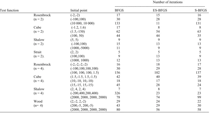
Table 1: Numerical results produced by the three tested algorithms, BFGS without scaling (BFGS), with Eigenvalue Scaling (ES-BFGS) and with step size scaling (S-BFGS)
Number of iterations
---
Test function Initial point BFGS ES-BFGS S-BFGS
Rosenbrock (-2,-2) 17 15 16
(n = 2) (-100,100) 30 28 28
(10 000, 10 000) 133 11 131
Cube (-1.2, 1.6) 17 8 8
(n = 2) (1.5,-150) 62 54 63
(100, 50) 44 44 35
Shalow (5, 5) 9 9 9
(n = 2) (-100,100) 15 13 13
(1000,-5000) 11 9 9
Strait (2, 2) 5 5 5
(n = 2). (100,100) 9 13 9
(1000, 1000) 12 13 13
Rosenbrock (-2,-2,-2,-2) 16 18 17
(n = 4). (-100,100,100,100) 30 29 28
(100, 100, 100, 1.5) 156 102 137
Cube (1.5,-1.5, 1.5,-1.5) 42 40 39
(n = 4). (10,-10, 10,-10) 18 17 18
(15,-15, 15,-15) 45 28 24
Shalow (2, 4, 2, 4) 7 8 7
(n = 4) (-200,400,200,400) 326 23 23
(2000, 2000, 2000, 2000) 78 74 99
Wood (2,-2, 2,-2) 29 24 22
(n= 4) (200,-5, 200,-5) 43 29 30
(2000, 2000, 2000, 2000) 80 56 58
DISCUSSION
From the calculation using MAPLE software, an interesting relation between step size and eigenvalues is observed. For initial iteration, the value of step size and the smallest eigen value of Hessian approximation is almost identical, but after a number of iterations, the difference increased accordingly. This explains why the ES-BFGS is effective on initial scaling only, a similarity with the scaled algorithm proposed by Shanno and Phua (1978). When the scaling on Hessian approximation was done on every iteration, the performance of the scaled BFGS deteriorated, or even failed at all.
The numerical results show that the new algorithm (ES-BFGS) performance is comparable to the algorithm with initial scaling (S-BFGS).
CONCLUSION
An improvement over unscaled BFGS is achieved, as for most of the cases (18 out of 24), the number of iterations are reduced. Further investigation will be carried out using the alternative scaling factor, λ on the other types of quasi-Newton methods. The relationship between the smallest eigenvalue of Hessian approximation and the optimal step size is also of the interest in future research, triggering the possibility of
using eigenvalue as a new step size in the quasi-Newton methods.
For every test function, the minimum point is (0,0) for the two variables functions and (0,0,0,0) for the four variables functions . The minimum value
is equal to zero for all the test functions. REFERENCES
Byrd, R.H., J. Nocedal and J. Y.X Yuan, 1987. Global convergence of a class of quasi-newton methods on Convex problems. SIAM J. Numer. Anal., 24: 1171-1189. DOI: 10.1137/0724077
Byrd, R.H. and J. Nocedal, 1989. A tool for the analysis of quasi-Newton methods with application to unconstrained minimization. SIAM J. Numer. Anal., 26: 727-739. DOI: 10.1137/0726042
Dennis, J.E. and J.J. More, 1977. Quasi-Newton methods, motivation and theory. SIAM Rev., 19: 46-89. DOI: 10.1137/1019005
Oren, S.S. and D.G. Luenberger, 1974. Self-scaling Variable Metric (SSVM) algorithms. Manage. Sci.,
20: 845-862. URL: http://.www.jstor.org/stable/2630094
Oren, S.S., 1973. Self-scaling variable metric algorithms without line search for unconstrained minimization. Math. Comput. Am. Math. Soc.,
Sun, W. and Y.X. Yuan, 2006. Optimization Theory and Method. Springer Optimization and Its Applications. 1st Edn., New York USA., ISBN: 10:0-387-24975-3, pp: 273-282.