Structural Path Analysis of Fossil Fuel Based CO2 Emissions: A Case Study for China.

(1)

Structural Path Analysis of Fossil Fuel Based

CO

₂

Emissions: A Case Study for China

Zhiyong Yang1,2, Wenjie Dong1,2, Jinfeng Xiu1, Rufeng Dai1,2, Jieming Chou1,2*

1State Key Laboratory of Earth Surface Processes and Resource Ecology, Beijing Normal University, Beijing, People’s Republic of China,2Future Earth Research Institute, Beijing Normal University Zhuhai, Zhuhai, Guangdong Province, People’s Republic of China

*choujm@bnu.edu.cn

Abstract

Environmentally extended input-output analysis (EEIOA) has long been used to quantify global and regional environmental impacts and to clarify emission transfers. Structural path analysis (SPA), a technique based on EEIOA, is especially useful for measuring significant flows in this environmental-economic system. This paper constructs an imports-adjusted single-region input-output (SRIO) model considering only domestic final use elements, and it uses the SPA technique to highlight crucial routes along the production chain in both final use and sectoral perspectives. The results indicate that future mitigation policies on house-hold consumption should change direct energy use structures in rural areas, cut unreason-able demand for power and chemical products, and focus on urban areas due to their consistently higher magnitudes than rural areas in the structural routes. Impacts originating from government spending should be tackled by managing onsite energy use in 3 major service sectors and promoting cleaner fuels and energy-saving techniques in the transport sector. Policies on investment should concentrate on sectoral interrelationships along the production chain by setting up standards to regulate upstream industries, especially for the services, construction and equipment manufacturing sectors, which have high demand pulling effects. Apart from the similar methods above, mitigating policies in exports should also consider improving embodied technology and quality in manufactured products to achieve sustainable development. Additionally, detailed sectoral results in the coal extrac-tion industry highlight the onsite energy use management in large domestic companies, emphasize energy structure rearrangement, and indicate resources and energy safety issues. Conclusions based on the construction and public administration sectors reveal that future mitigation in secondary and tertiary industries should be combined with upstream emission intensive industries in a systematic viewpoint to achieve sustainable develop-ment. Overall, SPA is a useful tool in empirical studies, and it can be used to analyze national environmental impacts and guide future mitigation policies.

OPEN ACCESS

Citation:Yang Z, Dong W, Xiu J, Dai R, Chou J (2015) Structural Path Analysis of Fossil Fuel Based CO2Emissions: A Case Study for China. PLoS ONE

10(9): e0135727. doi:10.1371/journal.pone.0135727

Editor:Aijun Ding, Nanjing University, CHINA

Received:November 15, 2014

Accepted:July 25, 2015

Published:September 2, 2015

Creative Commons Attribution License, which permits unrestricted use, distribution, and reproduction in any medium, provided the original author and source are credited.

Data Availability Statement:(1) 2007 Input-output table is available from the URL:http://tongji.cnki.net/ kns55/Navi/HomePage.aspx?id=

(2)

Introduction

According to recent studies, the concentration of carbon dioxide (CO2) in the atmosphere has

increased from approximately 277 parts per million (ppm) in 1750 [1] to 392.52 ppm in 2012 [2], and the average concentration exceeds 400 ppm for the first time in May 2013 [3]. Most of this growth since the industrial era can be ascribed to anthropogenic greenhouse gas (GHG) emissions, especially CO2from fossil fuel combustion and cement production. These CO2

emissions have been 8.6 ± 0.4 GtCyr-1on average during the past decade (2003–2012), three times the emission rates of the 1960s [4]. However, emission growth trends vary by nation and region. Developed countries (e.g., the US and western European countries) always show mod-erate CO2growth, whereas developing countries (e.g., China) have increased their emission

significantly in past decades [5]. Moreover, the magnitudes of CO2emissions in developed

countries have far surpassed those in developing countries since 1750, but in recent years, this trend has reversed [5]. All of these phenomena are highly correlated with the unprecedented expansion (more than 50%) of global energy demand since 1990, and in particular correlated with the rapid demand growth in non-Organization for Economic Cooperation and Develop-ment (non-OECD) countries since 2000 when China alone accounts for more than half of the increase [6]. Around 2011, China becomes the top CO2emitter from both producer and

con-sumer perspectives [7]. At the same time, most cities in North China are experiencing severe air pollution—annual particulate-matter (PM10) levels are 5–7 times the World Health

Organi-zation (WHO) guideline level [6], and annual sulfur dioxide (SO2) levels are triple the WHO

24-hour guideline level [8]. Together with global warming, these issues have caused growing public concerns, pushing fossil fuels (especially coal) to the top of the domestic political agenda, such as the five major actions on energy policy called for by Chinese President Jinping Xi in June 2014 [9]. Recently, China has declared a goal of reaching peak emissions before 2030, which indicates a sharp decrease in coal consumption and soaring demand for renew-ables [10]. Therefore, this work focuses on CO2emissions from fossil fuels in China and tries

to derive sound national and sectoral policies for future mitigation.

Often, input-output analysis (IOA) is used to analyze an economy in a structural way, con-sidering both intermediate and final use. EEIOA, as an extended IOA, is a methodology that combines IOA with environmental externalities. Both single-region input-output (SRIO) and multi-region input-output (MRIO) versions of EEIOA have been implemented, concentrating on embodied emissions in international trade [11–12], emission responsibilities in producer, consumer and shared perspectives [13–19] and other studies about water footprint and biodi-versity [20–21]. Another significant feature of EEIOA is its ability to display intricate sectoral inter-relationships along the production chain. The technique to excavate these linkages using EEIOA is called structural path analysis (SPA), which is often used in economics and regional science to analyze flows of energy, carbon, water and other physical quantities through indus-trial networks [22,23–26]. Moreover, SPA can be combined with structural decomposition analysis (SDA) to do deeper analysis, such as structural path decomposition (SPD) [27–28]. Currently, most CO2emission studies for China focus on major driving forces by using the

index decomposition method [29–30] or the structural decomposition method [31–34]. Rele-vant studies also analyze embodied emissions in bilateral trade [35–36] and assign emission responsibilities in different perspectives [37]. However, few have focused on emission interac-tions between different sectors along the production chains, such as Huang et al. [23] and Len-zen et al. [14]. Therefore, in this paper, we set up the first quantitative study for China using the SPA method to extract and analyze CO2emissions along the production chains from both

sectoral and final use perspectives based on imports-adjusted national input-output tables.

conversions/HS%20Correlation%20and% 20Conversion%20tables.htm.

Funding:This work is funded by the National Basic Program for Global Change Research of China (2012CB9557,http://www.973.gov.cn/Default_3. aspx), the National Natural Science Foundation of China (41175125 and 41330527,http://www.nsfc.gov. cn/), and the National level Major Incubation Project of Guangdong Province, China (2014GKXM058,

http://govinfonew.nlc.gov.cn/gdfz/govShow2015-01-6143086-TC0000000004.htm). The funders had no role in study design, data collection and analysis, decision to publish, or preparation of the manuscript.

(3)

The aim of this article is to understand the emission structures and the interdependence of sectors along the production chain and to derive sound policy for future mitigation. The remainder of this paper is arranged as follows: Section 2 describes the methods and materials used; Section 3 presents empirical studies with two different perspectives and discusses relevant policies; and Section 4 concludes the work and summarizes the implications.

Materials and Methods

Input-Output Analysis (IOA) and Import Assumptions

Based on the 2007 input-output (IO) table for China, a model is constructed to describe the total output of an economy:

X_¼AX_þC_þI_þG_þEX IM_þERR _ð₁_Þ

where X is the total output, A is the direct requirement matrix, C is household consumption, I is investment, G is government spending, EX is exports, IM is imports, and ERR is the error item that is included for balance and is provided in the IO table. Solving this Eq (1) for X gives:

X_{¼ ð}I A_Þ 1_ðC_þI_þG_þEX IM_þERR_{Þ ¼}L_ðC_þI_þG_þEX IM_þERR_{Þ ð}₂_Þ

where L represents the Leontief inverse matrix and X is the same as that given in (1). Combin-ing X with the environmental intensity row vector F, which represents CO2emissions per unit

of sector output in this study, total CO2emissions (EM) can be formulated as follows:

EM_¼FX_¼FL_ðC_þI_þG_þEX IM_þERR_Þ _ð₃_Þ

This is the so-called environmentally extended input-output model (EEIOA).

There is no doubt that an MRIO model is more appropriate than an SRIO model for esti-mating the actual carbon emissions embodied in trade because differences in environmental intensities and production chain structures in various nations are built into one model [38– 39]. Using MRIO with SPA makes it possible to simultaneously consider the global production chain and calculate detailed importing emissions originating from domestic final use [24–25,

38]. Nevertheless, construction of an integrated MRIO model is difficult due to data availabil-ity, time, various assumptions and harmonization work. An SRIO model, in contrast, is often self-contained, and the relevant data can be readily collected. Using competitive SRIO (as dis-cussed below) with SPA [14,23], it is also possible to consider the global production chain, although detailed importing sources are unavailable. In general, no universally superior model exists, there are only models that are more or less appropriate for specific purposes [39–41]. If the purpose is to analyze the incurred impacts from domestic produtive activities (namely C, I, G and EX excluding importing elements) and the sectoral inter-relationship along the domestic production chain, an SRIO model may be more appropriate due to data availability and computational resources. It is also reasonable to use an SRIO model because real transac-tions between industries usually can be assumed to happen within a nation, although incurred emissions might transcend the boundaries. Due to these facts, an adjusted SRIO model with 56 sectors for 2007 Chinese economy is used in this paper.

(4)

“direct requirement matrix”in competitive IO table is also called the“regional technical coefficients matrix”, and it includes intermediate use imports and can describe the real technol-ogy interrelationship of regional industries [42]. In contrast, the assumption behind direct requirement matrix in non-competitive IO table cannot accurately describe the technology of regional firms; rather, it describes the way in which local firms use local inputs [42]. Further-more, the competitive imports assumption in SRIO implies that the environmental intensities and supply chain structures in foreign nations are the same as those in the country being analyzed [38–39]. This is often called“Domestic Technology Assumption”(DTA) [44], the

“import assumption”[45–46] or the“single region assumption”[47]. Although this might cause errors in emissions embodied in imports [24,44–45,48–49], it is still supposed to be a balanced result considering time horizon, type of data, cost and work effort, detail and compre-hensiveness [50]. Because our purpose is to grasp the real interrelationship between industries along the production chain, we use the“regional technical coefficients”and the corresponding competitive imports assumption.

SRIO studies for China often treat imports as goods or services produced abroad, and many of them fail to distinguish between final uses that come from domestically produced (C1, I1, G1,

EX1) and imported (C2, I2, G2,EX2) sources [32–33], or they may simply assume that each

eco-nomic sector and final demand category uses imports in the same proportions [36,51]. Because our purpose is to see the incurred impacts from domestic final use, imports should be sub-tracted. Therefore, some elements in EX and IM are first eliminated (such as EX2), then 2007

Custom statistics in China are used to subtract the importing elements (C2, I2, G2) from the

remaining C, I and G. After removing all these importing elements from final use and imports (IM), we deriveEq 4:

EM_¼FX_¼FL_ðC₁_þI₁_þG₁_þEX₁ IM₁_þERR_Þ _ð₄_Þ

where IM1is imports for intermediate use. This modiﬁed IO table and Eq (4) can display actual

domesticﬁnal use and real inter-dependence of industries simultaneously.

Structural path analysis (SPA)

The Leontief inverse can be expanded using a power series approximation [52], and if we treat (C1+I1+G1+EX1-IM1+ERR) as a single vector Z, then

EM_¼F_ðI A_Þ 1Z_¼FIZ_þFAZ_þFA2

Z_þFA3

Z_þ _ð₅_Þ

where FAtZ represents the impact from tthproduction tier. For example, if Z represents a demand on the production of a plane, then FIZ is the direct manufacturer pollution from the production process. To produce this plane, inputs AZ from other industries are required, and FAZ of pollution is emitted. In turn, these industries require inputs of A2Z and emit FA2Z of pollutant. This process continues through the inﬁnite expansion of the power series. Finally, the whole picture of pollution derived from the production of the plane is drawn, and the shape is similar to a“tree data structure”in computer science.

Similar to the classical“80–20 Rule”, top several tiers contribute most of the influences, and within each tier, a limited number of nodes and routes are of great importance [14,53]. The

(5)

chain is referred to as Structural Path Analysis (SPA) [54]. Combined SPA with the selected depth of tiers, a cut-off threshold can be implemented to screen nodes above a certain level, thus setting up the boundaries of extraction. This is also called the“pruning method”[24–26,

53,55]. In this paper, sectors and routes are described using short English descriptors (see Table A inS1 File). For instance,“Power”and“Constr”represent the power sector and con-struction sector, respectively, and“Constr-Power”is the emission route originating from the power sector to satisfy downstream construction demands.

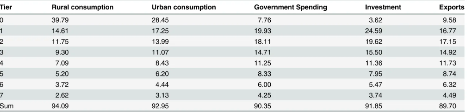
Table 1reveals that the first 8 tiers contribute nearly 90% of the total emissions for each domestic final use item. Tier 0 contributes most in rural and urban consumption, and Tiers 1 and 2 contribute the largest shares in investment, government spending and exports. This indicates that, for consumption, most emissions are embodied in direct purchase. For exports, investment and government spending, the majority of emissions originate from upstream sectoral interactions in the first several tiers. Based on existing studies, the depth of the tier number selected lies between 5 and 10 [24–26,53,56–57] and the cut-off threshold can be dis-played either in exact values [56–57] or in percentages, commonly ranging from 0.001% to 1% [14,23–26,53]. In this paper, the largest tier number is 8, and 0.001% is chosen as the cut-off threshold.

Data preparation

Two types of data are needed: the IO table and the CO2emission data by sector. The National

Bureau of Statistics of China (NBS) publishes a series of detailed basic IO tables for the Chinese economy in 1992, 1997, 2002 and 2007. The 135-sector symmetric IO table (in producer price) for 2007 is selected from the INPUT-OUTPUT TABLES OF CHINA [58] and is aggregated into 56 sectors (see Table B inS1 File) to carry out the empirical study. This aggregation method aims to harmonize both the economic sectoral data and energy sectoral data, and at the same time reflect enough details satisfying the purpose of our research. For example, the 27 sectors (“96–107”) in 135-sector IO table are aggregated into 8 sectors (“39–46”) in 56-sec-tor IO table (see Table B inS1 File) in order to match the“42”sector in energy statistics, as shown in Table C inS1 File.

General Administration of Customs (GAC) of China classifies the total merchandise trade into 19 sub-groups, including general trade, processing trade, inbound and outbound goods in bonded warehouses and storage of transit goods in bonded zones [59]. According to the defini-tions in INPUT-OUTPUT TABLES OF CHINA, EX and IM are total exports and imports, Table 1. Contribution of top 8 tiers to incurred emissions from each final use element (%).

Tier Rural consumption Urban consumption Government Spending Investment Exports

0 39.79 28.45 7.76 3.62 9.58

1 14.61 17.25 19.93 24.59 16.77

2 11.75 13.99 18.11 19.62 17.15

3 9.30 11.07 14.71 15.50 14.92

4 7.09 8.43 11.25 11.36 11.73

5 5.20 6.20 8.33 7.95 8.74

6 3.72 4.44 6.00 5.47 6.32

7 2.62 3.13 4.25 3.74 4.49

Sum 94.09 92.95 90.35 91.85 89.70

Direct household emissions are included in tier 0 of the rural or urban consumption. And investment is the sum ofﬁx capital formation and inventory change.

(6)

minus the processing trade values [58]. In order to achieve domestic final use elements, the value of goods imported and exported in bonded warehouses or zones is first separated from IM and EX (for merchandise trade sectors, 1–34), respectively, because these goods under bond administration are mainly preserved in the bonded warehouse or processed for export and will not enter domestic economic circulation [41]. The other three importing sub-groups (processing imported equipment, imported commodities and equipment as investment of foreign enterprises and imported equipment for export processing zones) are kept separate from the value of capital formation in sectors 1–34 because they are mainly used for investment purpose and are not generally used by households or government spending. The remaining imported goods in IM are separated into intermediate inputs and final use elements (excluding exports) using two methods. (1) For sectors 1–37, detailed merchandise imports in Harmo-nized System (HS) codes (version 2007) are selected from the China Customs Statistical Year-book [59]. Combining these data with the mapping relationships (from sectors to HS codes) in Sheng [60] and the Broad Economic Categories version 4 [61], we can get the proportions of intermediate goods, capital goods and consumption goods in these 37 sectors (see Table D and Figure A inS1 File). Using these proportions, imported elements in capital goods and con-sumption goods are eliminated from C, I and G. (2) For sectors 38–56, imports are prorated according to values of intermediate and final use elements (excluding exports) in each IO sec-tor, and those allocated to final use are subtracted from C, I and G. Finally, the modified IO table can display domestic final use and real production chains at the same time, which is dif-ferent from both the non-competitive and competitive IO tables.

CO2emissions data by sector are constructed using data from the Energy Statistics

Year-book [62]. Final energy consumption by industry sector in physical units and energy balance sheet in physical units [62] are combined and then transformed into energy units using net cal-orific values based on the GHG Protocol Tool for Energy Consumption in China (GPTFEC) [63]. This makes it possible to display sectoral energy consumption. Energy used for transfor-mation, energy losses and non-energy uses are all considered by using the procedures in Peters et al. [64]. Finally, sectors are aggregated or separated to match those in the 56-sector IO table (see Table C inS1 File), and energy combusted is transformed to CO2emissions using the

ref-erence method [65] based on the fraction of carbon oxidized and carbon content parameters in GPTFEC [63]. Total fossil fuel based CO2emissions from both industrial and household direct

use are calculated to be 6158.72 million metric tons (Mt). This is similar to 6112.42 Mt from the Carbon Dioxide Information Analysis Center (CDIAC) [66] and 6326.37 Mt from the U.S. Energy Information Administration [67], which testifies to the validity of this method.

Results and Discussion

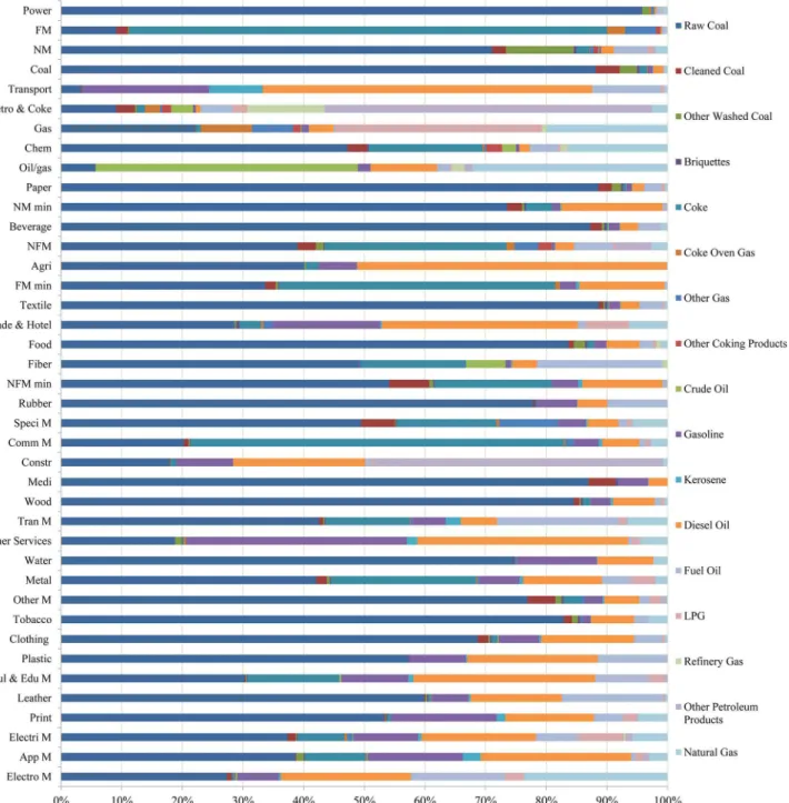
Considering sectoral emission intensities (seeFig 1), the largest one comes from power sector (951 g CO2/100 Yuan), which consumes almost four times as much as the FM sector. The

fol-lowing eight sectors have intensities greater than 50 g CO2/100 Yuan: NM, Coal, Transport,

(7)

emissions, whereas fuel oil, gasoline and diesel oil dominate the remaining share. For emissions in the Coke & Petro and Constr sectors, other petroleum products, refinery gas and oil prod-ucts contribute the most. Sectoral emissions in Gas and Oil/gas highly depend on LPG, natural gas and crude oil due to their industrial characteristics. The Electon M sector is the only equip-ment manufacturing sector that has the lowest emission share in coal and highest share in nat-ural gas. Tertiary industry can be summarized to three sectors due to our aggregation and Fig 1. Sectoral emission intensity structures categorized in 17 final energy forms.The vertical axis shows 40 sectors in the descending order of their emission intensities from top to bottom. The horizontal axis shows the percentages of 17 final use energy forms for each sector. The transport sector includes Rail T, Land T, Water T, Air T, Pipe T, Public T, Storage and Post. Other services include all tertiary industries, except those in the transport sector (above) and the Trade & Hotel sector (namely Trade sector and Hotel sector).

(8)

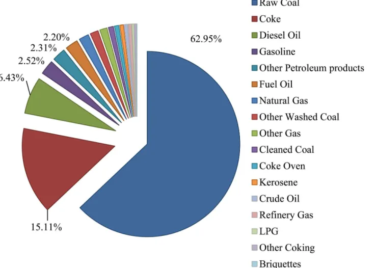
disaggregation methods (see Tables B and C inS1 File): Transport sector, Hotel & Trade sector and Other services sector. Gasoline, kerosene, diesel oil and fuel oil dominate the emissions in transport sector, whereas raw coal, gasoline and diesel oil dominate the other two sectors. Taking all sectors together, the shares of CO2from final energy consumed in 2007 are shown

inFig 2. Raw coal (62.95%) is the most important final energy form in China, coke (15.11%) is the second and is highly required in metal smelting and machine manufacturing, and diesel oil (6.43%) is third; it is particularly popular in Transport, Agri and Other service sectors.

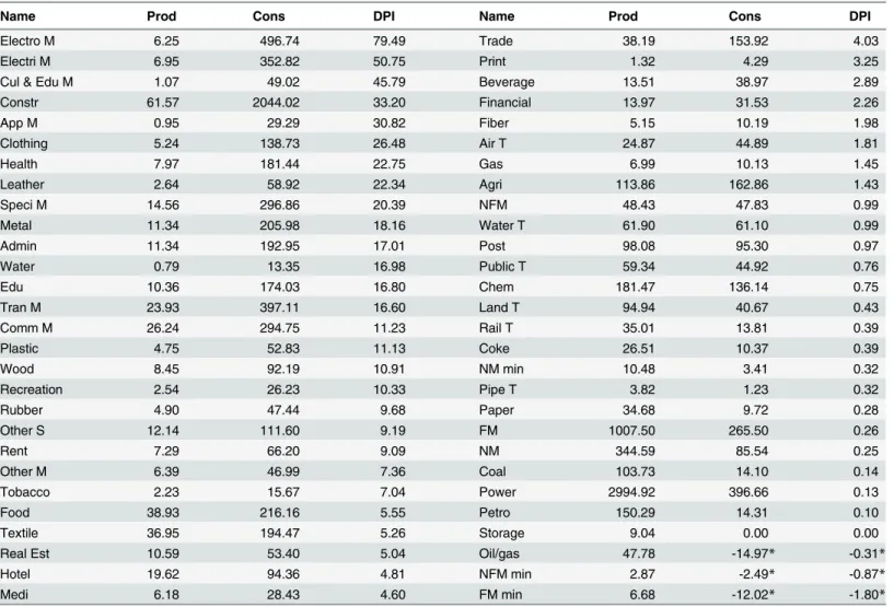
To compare production-based emissions and incurred consumption-based emissions from final use sectors, we define the ratio of incurred emissions to production-based ones as

“demand pulling indicator (DPI)”. DPI = 1 means sectoral emissions in production are equilib-rium with those in consumption; DPI<1 implies that this sector contributes more to satisfy-ing other sectors’demand than its own needs in the production chain; DPI>_{1 indicates this} sector depends on more emissions from other sectors in the production chain than its own pro-duction to satisfy its own demand. DPI is an indicator of sectoral roles (supplier or demander) in the production chain.Table 2displays DPI values for 56 sectors. Power generation (Power), resource extraction (e.g., FM min, NM min, NFM min, Coal and Oil/gas), resource processing (e.g., FM, NM, Paper, Petro) and transport (e.g., Land T, Rail T and Public T) dominate the Fig 2. Percentages of CO2emissions from different final energy forms in 2007 for China.Each sector in the pie chart represents the emission

percentage of one type of final energy.

(9)

DPI indicators lower than 1, which means they are supporting other sectors in the production chain. Except for 3 sectors (NFM, Post and Water T) with DPI values around 1, all other 36 sectors have DPI values greater than 1. Equipment manufacturing sectors (e.g., Electro M, App M, Speci M) show significantly large DPI values ranging from 7.63 to 79.49. Construction (DPI = 33.20), Clothing (DPI = 26.48), Metal (DPI = 18.16) and various services sectors (e.g., Health, Edu, Real Est and Hotel) are also significant. It is clear that all of these 36“demanding”

sectors belong to downstream manufacturing industries or services and they are highly depen-dent on upstream transport, resources and power sectors. Downstream sectors with large DPI values can have a strong demand pulling effect on economy and emissions, and therefore, they should be treated seriously.

Based upon the analyses above, we have drawn a basic picture of the sectoral emission pat-terns and their inter-relationship in the production chain. To further clarify the incurred CO2

emissions from a structural viewpoint and to develop sound mitigation policies, the SPA tech-nique is implemented in both final use and sectoral perspectives in the following sections. Table 2. Production-based emissions, consumption-based emissions and DPI indicators for 56 sectors in 2007.

Name Prod Cons DPI Name Prod Cons DPI

Electro M 6.25 496.74 79.49 Trade 38.19 153.92 4.03

Electri M 6.95 352.82 50.75 Print 1.32 4.29 3.25

Cul & Edu M 1.07 49.02 45.79 Beverage 13.51 38.97 2.89

Constr 61.57 2044.02 33.20 Financial 13.97 31.53 2.26

App M 0.95 29.29 30.82 Fiber 5.15 10.19 1.98

Clothing 5.24 138.73 26.48 Air T 24.87 44.89 1.81

Health 7.97 181.44 22.75 Gas 6.99 10.13 1.45

Leather 2.64 58.92 22.34 Agri 113.86 162.86 1.43

Speci M 14.56 296.86 20.39 NFM 48.43 47.83 0.99

Metal 11.34 205.98 18.16 Water T 61.90 61.10 0.99

Admin 11.34 192.95 17.01 Post 98.08 95.30 0.97

Water 0.79 13.35 16.98 Public T 59.34 44.92 0.76

Edu 10.36 174.03 16.80 Chem 181.47 136.14 0.75

Tran M 23.93 397.11 16.60 Land T 94.94 40.67 0.43

Comm M 26.24 294.75 11.23 Rail T 35.01 13.81 0.39

Plastic 4.75 52.83 11.13 Coke 26.51 10.37 0.39

Wood 8.45 92.19 10.91 NM min 10.48 3.41 0.32

Recreation 2.54 26.23 10.33 Pipe T 3.82 1.23 0.32

Rubber 4.90 47.44 9.68 Paper 34.68 9.72 0.28

Other S 12.14 111.60 9.19 FM 1007.50 265.50 0.26

Rent 7.29 66.20 9.09 NM 344.59 85.54 0.25

Other M 6.39 46.99 7.36 Coal 103.73 14.10 0.14

Tobacco 2.23 15.67 7.04 Power 2994.92 396.66 0.13

Food 38.93 216.16 5.55 Petro 150.29 14.31 0.10

Textile 36.95 194.47 5.26 Storage 9.04 0.00 0.00

Real Est 10.59 53.40 5.04 Oil/gas 47.78 -14.97* -0.31*

Hotel 19.62 94.36 4.81 NFM min 2.87 -2.49* -0.87*

Medi 6.18 28.43 4.60 FM min 6.68 -12.02* -1.80*

*These negative values inConsandDPIcan be ascribed to negative values inventory change.

(10)

Final use perspective

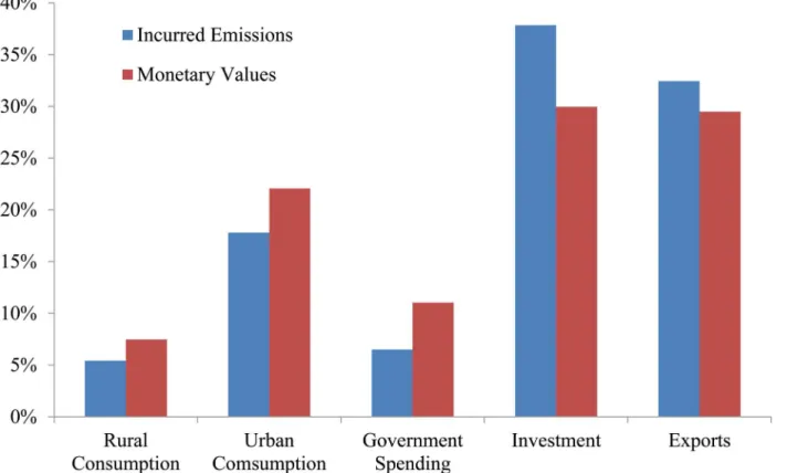
The bar chart inFig 3reveals monetary and incurred emission ratios of each domestic final use element. Similar to the monetary ratios, exports and investment dominate the total incurred emissions, but they are more emission intensive because they have higher ratios of incurred emissions than monetary values. This can be ascribed to large flows of investment in 2007 going to manufacturing sectors (32.41%), real estate (23.62%), transport, storage and post (10.31%) and public infrastructure and facilities (7.39%), which all have high DPI values [68]. Exports in 2007 mainly flow to equipment manufacturing (47%) and“textiles, light industrial products, rubber products, minerals and metallurgical products”(18%), which also have large DPI values [68]. Moreover, the low DPI values and large monetary amounts of services sectors (e.g., Admin, Land T and Public T) in government spending and household consumption can partly explain their lower emission ratios than monetary ones. Tables3–7demonstrate 25 top-ranking paths for CO2originating from the household (rural and urban) consumption,

invest-ment, government spending and exports. All of these top paths are ranked in descending order due to their contributions to incurred emissions.

Household consumption

Household emissions from direct energy use (Tables3and4) in rural and urban areas contrib-ute 126.16 Mt and 140.48 Mt CO2, respectively. The ratio of direct use emissions to total

emis-sions from household consumption activities in rural area is quite large (23.35%), but the ratio in urban areas is only 9.36%. The reason for this huge difference is the energy use structures in Fig 3. Shares of incurred emissions and monetary values from five domestic final use items.Red bar charts represent the percentages of monetary values, and blue bar charts represent ratios of incurred emissions. Investment is the sum of fix capital formation and inventory change. Direct household emissions are not included in the household emissions.

(11)

these two areas. As shown inFig 4, rural areas depend greatly on raw coal and briquettes, whereas urban areas rely heavily on gas fuels. Therefore, mitigation policy towards household direct use emissions should focus on the energy structure in rural areas and raise the share of gas fuels and renewable energy sources, such as solar and biomass.

For the top 25 routes originating from indirect energy use in both rural and urban areas (see Tables3and4), these emissions account for 25%-29% of total emissions from household con-sumption activities. Many top routes exist as onsite emissions, which have lengths of one and come from direct purchases of final demand (e.g.,“Power”,“Agri”,“Post”and“Food”). The largest onsite emissions occur in the demand for electricity and heat (“Power”), which can be ascribed to high dependence on coal for power generation in China. Other onsite emissions lie in food, transportation, agriculture, trade services and real estate sectors, in which urban areas have higher emission values by a factor of 3 to 6 compared to rural areas. Comparisons between top routes in Tables3and4indicate that chemical sector is rather specific for rural consump-tion because“Agri-Chem”and“Agri-Chem-Power”only exist inTable 3. Due to our classifica-tion, Chem includes seven subsectors (see Table B inS1 File) and Agri includes five subsectors in the original 135 IO table [58]. Focusing on the monetary flows from subsectors in Chem to Table 3. Top 25 routes of CO2emissions from Rural household Consumption.

Ranks Data (Mt CO2) Ratio (%) Routes

0 126.16 23.35% Direct energy use

1 48.27 8.93% Power

2 17.31 3.20% Power—Power

3 11.89 2.20% Agri

4 6.21 1.15% Power—Power—Power

5 5.26 0.97% Post

6 4.55 0.84% Agri—Power

7 3.80 0.70% Edu—Power

8 3.78 0.70% Food

9 3.38 0.63% Food—Power

10 3.31 0.61% Food—Agri

11 3.02 0.56% Hotel—Power

12 2.98 0.55% Trade—Power

13 2.73 0.51% Trade

14 2.23 0.41% Power—Power—Power—Power

15 2.11 0.39% Agri—Chem—Power

16 1.85 0.34% Agri—Chem

17 1.67 0.31% Agri—Agri

18 1.66 0.31% Hotel

19 1.63 0.30% Agri—Power—Power

20 1.63 0.30% Real Est

21 1.55 0.29% Land T

22 1.36 0.25% Beverage

23 1.36 0.25% Edu—Power—Power

24 1.32 0.24% Water T

25 1.28 0.24% Public T

SUM 136.14 25.18% —

SUM in the last row refers to the sum ofﬁgures ranking from 1 to 25.

(12)

Agri, we find that chemical fertilizer and chemical pesticides are the most significant. Interme-diate flows from the fertilizer sector to the agriculture sector are more than six times greater than those from the pesticide sector. Therefore, CO2emissions from fertilizer and pesticide

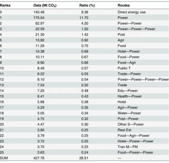
production in Chem contribute greatly to satisfying rural consumption in Agri. And future mitigation policy should be implemented to limit the unreasonable dependence of agriculture on fertilizer and pesticides and to reduce emission intensities during these chemicals produc-tion. As for urban consumption, more emphasis is placed on education, health and other ser-vices, as shown inTable 4. Moreover, because the most indirect paths end up in the Power sector, emissions intensity reduction and unreasonable downstream demand cuts in Power can be rather crucial for future mitigation policy. Overall, the results show that future policies should be implemented to change the direct energy use structures in rural areas, to reduce emission intensities and cut unreasonable demand in Power and Chem sectors, and to focus more on urban areas due to its higher magnitudes in the same routes.

Table 4. Top 25 routes of CO2emissions from Urban household Consumption.

0 140.48 9.36 Direct energy use

1 175.54 11.70 Power

2 62.97 4.20 Power—Power

3 22.59 1.50 Power—Power—Power

4 21.30 1.42 Post

5 13.82 0.92 Agri

6 11.29 0.75 Food

7 10.38 0.69 Hotel—Power

8 10.11 0.67 Food—Power

9 9.90 0.66 Food—Agri

10 8.49 0.57 Public T

11 8.22 0.55 Trade—Power

12 8.10 0.54 Power—Power—Power—Power

13 7.53 0.50 Trade

14 7.25 0.48 Edu—Power

15 6.41 0.43 Health—Power

16 5.68 0.38 Hotel

17 5.29 0.35 Agri—Power

18 5.05 0.34 Water—Power

19 4.75 0.32 Post—Power

20 4.47 0.30 Other S—Power

21 3.80 0.25 Real Est

22 3.79 0.25 Food—Agri—Power

23 3.72 0.25 Hotel—Power—Power

24 3.70 0.25 Tran M—FM

25 3.63 0.24 Food—Power—Power

SUM 427.76 28.51 —

SUM in the last row refers to the sum ofﬁgures ranking from 1 to 25.

(13)

Government Spending

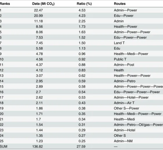
The top 25 routes inTable 5contribute 27.6% of the total incurred emissions by government spending. These incurred impacts are dominated by various transport modes (e.g., Land T and Public T) and service activities (mainly the Health, Edu and Admin sectors). Indirect routes are significant on the top list and more important than onsite routes. This is common for service sectors because these activities are often not energy intensive (as shown inFig 1), and they are supported by upstream emission intensive industries.Table 1further verifies this; the tier 1 ratio is three times the value of tier 0. For example, the Edu sector requires large amounts of power to operate schools and universities (DPI = 18.8) and hospitals in the“Health”sector need both energy and medical products to function well (DPI = 22.75). As for the Admin sector (e.g., administrative authorities at various levels), which is the largest expenditure item in gov-ernment spending, relevant environmental impacts mainly flow to transport (“Admin-Air T”), power generation (“Admin-Power”), post services (“Admin-Post”) and petroleum products manufacturing (“Admin-Petro”) sectors. To mitigate emissions originating from government spending, future policies should not only manage and supervise onsite energy use in these ser-vice sectors but also reduce emission intensities in upstream industries. As for transport sec-tors, since they are emission intensive, future policies should focus on promoting cleaner fuels (e.g., biomass and hydrogen), energy-saving techniques and publishing relevant transportation standards are also necessary, especially for Land T and Public T sectors.

Table 5. Top 25 routes of CO2emissions from Government Spending.

1 22.47 4.53 Admin—Power

2 20.99 4.23 Edu—Power

3 11.18 2.25 Admin

4 8.56 1.73 Health—Power

5 8.06 1.63 Admin—Power—Power

6 7.53 1.52 Edu—Power—Power

7 7.45 1.50 Land T

8 5.58 1.13 Edu

9 4.78 0.96 Health—Medi—Power

10 4.56 0.92 Public T

11 4.37 0.88 Admin—Post

12 4.12 0.83 Health

13 3.07 0.62 Health—Power—Power

14 2.95 0.59 Admin—Petro

15 2.89 0.58 Admin—Power—Power—Power

16 2.7 0.54 Edu—Power—Power—Power

17 2.62 0.53 Admin—Hotel—Power

18 2.11 0.43 Admin—Air T

19 1.86 0.38 Other S—Power

20 1.71 0.35 Health—Medi—Power—Power

21 1.7 0.34 Health—Medi

22 1.54 0.31 Admin—Petro—Oil/gas—Power

23 1.44 0.29 Admin—Hotel

24 1.35 0.27 Other S

25 1.23 0.25 Admin—NM

SUM 136.82 27.59 —

(14)

Investment

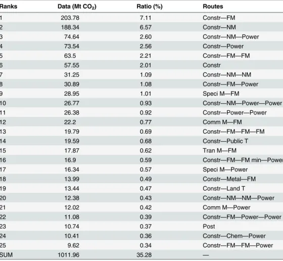
Investment includes both fixed capital investment and inventory change. Fixed capital invest-ment mainly flows to the real estate sector, the industrial sectors and infrastructure construc-tion activities. The magnitude of investment is always greater than the inventory change, and so are the emissions incurred. Top 25 routes contribute to 35.28% of total incurred emis-sions, as shown inTable 6. Apart from onsite emission routes ranking 6th(“Constr”) and 23rd (“Post”) on the list, all other routes originate from indirect purchases. Most of these indirect emissions stem from the demand for equipment manufacturing (Spec M, 7.75%, Comm M, 6.35% and Trans M, 9.1%) and construction activities (Constr, 57.4%), as shown in the aggre-gated 56-sector IO table. Often, these demand flow upstream along the production chain and end up in the ferrous metal smelting (FM) and non-metallic smelting (NM) sectors. Although the Power sector is also acting as a crucial end point in indirect routes for investment, it is not as significant as the routes for household consumption and government spending (see Tables

3–5). Combining these investments in the manufacturing and construction sectors with their large DPI values makes it clear that investment contributes a huge share (38%) of total incurred emissions (as shown inFig 1). Thus, future mitigation policies should focus on direct emission intensity reduction in the major investment sectors and establish standards to regulate their demand for emission intensive upstream materials (such as the demand for steel, glass and Table 6. Top 25 routes of CO2emissions from Investment.

1 203.78 7.11 Constr—FM

2 188.34 6.57 Constr—NM

3 74.64 2.60 Constr—NM—Power

4 73.54 2.56 Constr—Power

5 63.5 2.21 Constr—FM—FM

6 57.55 2.01 Constr

7 31.25 1.09 Constr—NM—NM

8 30.89 1.08 Constr—FM—Power

9 28.95 1.01 Speci M—FM

10 26.77 0.93 Constr—NM—Power—Power

11 26.38 0.92 Constr—Power—Power

12 22.2 0.77 Comm M—FM

13 19.79 0.69 Constr—FM—FM—FM

14 19.59 0.68 Constr—Public T

15 17.87 0.62 Tran M—FM

16 16.9 0.59 Constr—FM—FM min—Power

17 16.34 0.57 Speci M—Power

18 13.99 0.49 Constr—Metal—FM

19 13.44 0.47 Constr—Land T

20 12.38 0.43 Constr—NM—NM—Power

21 12.02 0.42 Comm M—Power

22 11.08 0.39 Constr—FM—Power—Power

23 10.74 0.37 Post

24 10.41 0.36 Constr—Chem—Power

25 9.62 0.34 Constr—FM—FM—Power

SUM 1011.96 35.28 —

(15)

concrete in Constr sector), especially for those sectors with large DPI values. This will help encourage emission reductions along the whole production chain.

Exports

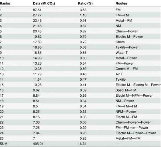
Table 7shows the top 25 routes resulting from exports, and cumulative emissions are only 16.34% of the total. Compared with other final use elements, this low share indicates that most emissions are dispersed along the production chain. As we can see fromTable 7, onsite emis-sions from the FM, NM, Textile, Water T, Air T and Chem sectors contribute a great deal. Indi-rect routes, however, mainly start from resource processing sectors (e.g., FM, NM, NFM, Chem and Metal) and equipment manufacturing sectors (e.g., Electri M, Speci M and Electro M and Comm M), and they end up in the two energy intensive sectors: ferrous metal smelting and pressing (FM) and power generation (Power). Additionally, research on embodied technology and quality of manufactured exports in China [69] indicates that low-technology products still dominated the manufactured exports (nearly 53%) in 2007, and shares of medium- (23%) and high-technology (11%) products keep growing, but are still lower than the global averages. Rel-evant quality results also indicate that most manufactured exports lie in low-quality areas (50.2%) [69].

In summary, exports in 2007 are mainly resource- or emission-intensive metal products, equipment manufacturing and chemical products, in which low technology and low quality Table 7. Top 25 routes of CO2emissions from Exports.

1 87.51 3.53 FM

2 27.27 1.10 FM—FM

3 22.46 0.91 Metal—FM

4 21.48 0.87 NM

5 20.45 0.82 Chem—Power

6 19.62 0.79 Electro M—Power

7 17.89 0.72 Chem

8 16.85 0.68 Textile—Power

9 16.85 0.68 Water T

10 14.93 0.60 Metal—Power

11 13.26 0.54 FM—Power

12 12.35 0.50 Comm M—FM

13 11.79 0.48 Air T

14 11.54 0.47 Textile

15 10.28 0.41 Electro M—Electro M—Power

16 9.62 0.39 Speci M—FM

17 8.84 0.36 Electri M—NFM—Power

18 8.51 0.34 NM—Power

19 8.5 0.34 FM—FM—FM

20 8.25 0.33 NFM—Power

21 8.16 0.33 Electri M—FM

22 7.33 0.30 Chem—Power—Power

23 7.26 0.29 FM—FM min—Power

24 7.04 0.28 Electro M—Power—Power

25 7 0.28 Metal—FM—FM

SUM 405.04 16.34 —

(16)

prevail. Therefore, future mitigation polices should pay attention to those intensive sectors, try to reduce their direct emission intensities, cut unreasonable demand, and improve the embod-ied technology and quality in manufactured goods by reshaping exports structures. In other words, future policies should combine environmental guidance with economic structural change.

Sectoral perspective

After discussing environmental impacts from different final use elements, three representative sectors with a wide variety of business types are selected to illustrate the further implications regarding interrelationships among industries: a large extractive industry (coal mining), a sig-nificant secondary industry (construction) and a tertiary industry (public administration). The emissions and ratios of the top 25 routes for specific sectors are shown in Tables8–11.

Coal Mining and Dressing Sector

Results show that 363.89 g of accumulated CO2are emitted for every 1 Yuan of final demand

in the Coal sector, and the top 25 routes account for 70% of the total incurred emissions (see

Table 8). Tracking these routes makes it possible to recognize the interrelationships between Coal and other sectors. Column 1 inTable 8shows the ranking positions of various routes, and column 2 refers to their incurred CO2emissions (in grams) by unit final demand in Coal

sec-tor. For example, route“Coal-Power”indicates that 59.4 g CO2is emitted due to fuel

combus-tion in electricity and heat generacombus-tion to serve unit final demand for the Coal sector. Column 3 represents ratios of these incurred emissions in each route to total ones. Column 4 shows route details along the production chain.

Fig 4. Shares of direct energy use in different forms for rural and urban areas in 2007.Blue and red bars represent ratios for urban and rural areas, respectively. All energy forms are measured in standard quantity (10,000 tons of coal equivalent).

(17)

A 30% share of total incurred emissions comes from onsite energy use, which is rather remarkable; it is almost twice the emissions of the second largest route. This means that the Coal sector contributes a great deal without depending on the upstream industries. Indirect routes indicate that the Coal sector depends greatly on the Power sector, as shown in the routes ranking 2, 3, 6, 9 and 23. It also relies on metal products (e.g., FM and Metal), equipment manufacturing (e.g., Speci M and Comm M) and transport (e.g., Land T and Water T), which can be ascribed to the construction of rigs/equipment and the transportation of coal products. What is more, exports contribute the most in the final demand for Coal sector, and this is quite different from other resource mining industries (FM min, NM min, NFM min, Oil/gas sectors) in which imports dominate.

Therefore, future mitigation policies should focus on energy use management in large domestic coal mining companies, for both fossil fuel combusted onsite and electricity and heat consumed along the production processes. Because raw coal is the major fuel (94.5%) used for generating electricity and heat (seeFig 1) [62], future policies also should focus on rearranging energy structures, limiting raw coal consumption and promoting other cleaner or renewable energy forms. Moreover, attention should be directed to resources and energy safety issues, especially for crude oil, gas, metal ores (e.g., FM min and NFM min) due to their huge imports in final demand. As for the huge exports in Coal sector, future policy should analyze benefits and costs considering the energy and environmental dilemmas in China.

Table 8. Top 25 routes for unit demand in Coal Mining & Dressing (“Coal”) Sector.

Ranks Data (g CO2) Ratio (%) Routes

1 107.55 29.56 Coal

2 59.40 16.32 Coal—Power

3 21.31 5.86 Coal—Power—Power

4 11.24 3.09 Coal—FM

5 10.82 2.97 Coal—Coal

6 7.64 2.10 Coal—Power—Power—Power

7 5.97 1.64 Coal—Coal—Power

8 3.50 0.96 Coal—FM—FM

9 2.74 0.75 Coal—Power—Power—Power—Power

10 2.24 0.62 Coal—Land T

11 2.14 0.59 Coal—Coal—Power—Power

12 1.70 0.47 Coal—FM—Power

13 1.55 0.43 Coal—NM

14 1.51 0.41 Coal—Metal—FM

15 1.28 0.35 Coal—Comm M—FM

16 1.18 0.32 Coal—Petro

17 1.13 0.31 Coal—Coal—FM

18 1.13 0.31 Coal—Speci M—FM

19 1.09 0.30 Coal—FM—FM—FM

20 1.09 0.30 Coal—Coal—Coal

21 1.06 0.29 Coal—Water T

22 1.00 0.28 Coal—Metal—Power

23 0.98 0.27 Coal—Power—Power—Power—Power—Power

24 0.93 0.26 Coal—FM—FM min—Power

25 0.93 0.25 Coal—Rail T

SUM 251.12 69.01 —

(18)

Construction Sector

Because investment flows into infrastructure development and real estate market have soared in recent years [68], the construction sector requires special focus. Similar to the Coal sector, the top 25 routes in the Constr (seeTable 9) sector account for half of total incurred emissions (48%), and the sectoral unit final demand can stimulate 340.9 g CO2. The results show that

onsite emissions are less significant (merely 2.88% of the total) and a majority of large emission routes originate from indirect purchases (such as“Constr-NM”and“Constr-Power”) flowing upstream to NM, FM and Power sectors. Other intensive sectors, such as chemical products (Chem), refinery products (Petro), metals (Metal) and transport services (Land T, Public T and Post) are also strongly required. Unlike the Coal sector, which belongs to upstream industry and has only a small DPI value (0.14), the downstream Constr sector has a great demand pulling effect (DPI value equals 33.2) on the total economy. Additionally, final demand for Constr mainly resides in fixed capital formation and barely shows in imports, as seen in the aggregated IO table, indicating that incurred emissions in this sector are mostly for domestic use. Therefore, future mitigation work should pay great attention to Constr and similar sectors that account for large shares of domestic emissions, especially those with large DPI values. Rel-evant sectoral policies should also focus on managing onsite energy use, promoting new build-ing technology, cuttbuild-ing unreasonable construction plans and settbuild-ing up new standards for upstream materials as declared in the“Investment”section above. Considering the booming Table 9. Top 25 routes for unit demand in Construction Sector.

1 34.76 10.20 Constr—FM

2 32.13 9.43 Constr—NM

3 12.73 3.74 Constr—NM—Power

4 12.54 3.68 Constr—Power

5 10.83 3.18 Constr—FM—FM

6 9.82 2.88 Constr

7 5.33 1.56 Constr—NM—NM

8 5.27 1.55 Constr—FM—Power

9 4.57 1.34 Constr—NM—Power—Power

10 4.5 1.32 Constr—Power—Power

11 3.38 0.99 Constr—FM—FM—FM

12 3.34 0.98 Constr—Public T

13 2.88 0.85 Constr—FM—FM min—Power

14 2.39 0.70 Constr—Metal—FM

15 2.29 0.67 Constr—Land T

16 2.11 0.62 Constr—NM—NM—Power

17 1.89 0.55 Constr—FM—Power—Power

18 1.78 0.52 Constr—Chem—Power

19 1.64 0.48 Constr—FM—FM—Power

20 1.64 0.48 Constr—NM—Power—Power—Power

21 1.61 0.47 Constr—Power—Power—Power

22 1.59 0.47 Constr—Metal—Power

23 1.57 0.46 Constr—Petro

24 1.55 0.46 Constr—Chem

25 1.38 0.41 Constr—Post

SUM 163.52 48 —

(19)

real estate markets and infrastructure development in China and their huge demand pulling effects on emission intensive upstream industries through Constr sector, future development policies in these two fields must combine economic concerns with environmental ones to achieve sustainable development.

Public Administration Sector

Unit final demand in the Admin sector can stimulate 123.4 g CO2along the production chain,

and the top 25 routes account for 37.7% of the total incurred emissions (seeTable 10). The largest incurred impacts mainly come from the indirect purchase route (“Admin—Power”), which contributes 11.68% of total emissions, whereas onsite emissions contribute 5.8%. Vari-ous tertiary sectors (e.g., Post, Transport, and Hotel) and secondary sectors (e.g., Constr, Petro and NM) are strongly required in the top 25 list. The DPI value for the public administration sector is 17, which is similar to other large service sectors, such as Edu (DPI = 16.8) and Health (DPI = 22.75). Moreover, final use in Admin sector mainly consists of government spending and is the largest cell in it, as shown in the original IO table. All of these facts remind us that future policies must not ignore service sectors due to their high pulling effects on emissions and the economy. Future policies should not only manage and supervise onsite energy use in these service sectors but also promote reduction of emission intensities upstream from a sys-tematic viewpoint.

Table 10. Top 25 routes for unit demand in Public Adminstration Sector.

1 14.41 11.68 Admin—Power

2 7.17 5.81 Admin

3 5.17 4.19 Admin—Power—Power

4 2.81 2.27 Admin—Post

5 1.89 1.53 Admin—Petro

6 1.85 1.50 Admin—Power—Power—Power

7 1.68 1.36 Admin—Hotel—Power

8 1.36 1.10 Admin—Air T

9 0.99 0.80 Admin—Petro—Oil/gas—Power

10 0.92 0.75 Admin—Hotel

11 0.79 0.64 Admin—NM

12 0.74 0.60 Admin—Petro—Oil/gas

13 0.67 0.54 Admin—Power—Power—Power—Power

14 0.63 0.51 Admin—Edu—Power

15 0.63 0.51 Admin—Post—Power

16 0.6 0.49 Admin—Hotel—Power—Power

17 0.55 0.45 Admin—Land T

18 0.51 0.41 Admin—Rail T

19 0.5 0.41 Admin—Constr—FM

20 0.49 0.40 Admin—Wood—Power

21 0.46 0.38 Admin—Constr—NM

22 0.46 0.38 Admin—Paper

23 0.45 0.37 Admin—Print—Paper

24 0.45 0.36 Admin—Tran M—FM

25 0.38 0.30 Admin—Air T—Petro

SUM 46.56 37.74 —

(20)

Additionally, we compare the above results with two other SPA studies from Peters and Hertwich [25] and Huang et al. [23] in both the final use and sectoral perspectives. In the final use viewpoint, our results resemble those tier distribution results in household consumption and government spending for Norway [25], but they are different from those results in exports. This difference can be explained by direct emissions from inter-national shipping and direct processing in the oil and gas sector, which are unique for Norway. As for incurred emission routes from each final use elements (household consumption, government spending and exports) [25], the differences are clear. China often ends up in emission intensive electricity and heat (Power) sector while Norway relies on transport sectors a lot, which can be ascribed to their very different energy structures. The Norwegian economy has low emission intensity due primarily to the use of hydropower in electricity generation, whereas the Chinese economy depends greatly on coal. Another significant difference lies in the export sector; Norway is dominated by international shipping and oil/gas production (over 40%) due to its resources, but China shows a distributing nature in many small routes for industrial products (e.g., metal, equipment manufacturing and chemicals). Additionally, routes in the final use viewpoint have much in common for the same economic reasons, such as high demand for Food and Agri products in household consumption and large requirements for Health, Edu and Admin ser-vices in government spending.

In the sectoral viewpoint, the Oil and gas extraction sector (Oil/gas) is chosen for demon-stration (seeTable 11). Unlike the environmental impacts used in this study, the impact indica-tor in Huang et al. [23] is GHG equivalents (CO2-eq), which includes CO2, CH4and other

GHGs. These incurred CO2-eq routes from unit sectoral demand in Australia and US are

com-puted using SRIO and SPA based on 2001 and 2002 IO table, respectively [23]. The results reveal that 67%, 89% and 93% of emissions come from the top 20 routes for China, Australia Table 11. Top 25 routes for unit demand in Oil/gas Extraction Sector.

1 66.59 23.84 Oil/gas—Power

2 50.11 17.94 Oil/gas

3 23.89 8.55 Oil/gas—Power—Power

4 12.33 4.42 Oil/gas—FM

5 8.57 3.07 Oil/gas—Power—Power—Power

6 3.84 1.38 Oil/gas—FM—FM

7 3.16 1.13 Oil/gas—Petro

8 3.07 1.10 Oil/gas—Power—Power—Power—Power

9 1.87 0.67 Oil/gas—FM—Power

10 1.65 0.59 Oil/gas—Petro—Oil/gas—Power

11 1.5 0.54 Oil/gas—Speci M—FM

12 1.41 0.50 Oil/gas—Chem—Power

13 1.3 0.46 Oil/gas—NM

14 1.24 0.44 Oil/gas—Petro—Oil/gas

15 1.23 0.44 Oil/gas—Chem

16 1.2 0.43 Oil/gas—FM—FM—FM

17 1.1 0.39 Oil/gas—Power—Power—Power—Power—Power

18 1.02 0.37 Oil/gas—FM—FM min—Power

19 0.95 0.34 Oil/gas—Comm M—FM

20 0.9 0.32 Oil/gas—Oil/gas—Power

SUM 186.93 66.92 —

(21)

and the US, respectively. The onsite emissions, which might occur directly at rig/drilling sites in the US and Australia, are quite high (85.2% and 80.9%), and China contributes just 18%. However, indirect emissions from the Power sector dominates the top ranks (nearly 24%) in China and is more significant than in the US (3%) and Australia (8%), which might be due to China’s high dependence on coal for electricity and heat. These huge differences might be due to different energy use patterns in the Oil/gas sector. Large demand for petroleum products, ferrous metals, equipment and machinery are all shown in top 20 routes of three target studies. In summary, our SPA results in two viewpoints show both common results to earlier studies and special characteristics due to China’s own economic and energy structures. Therefore, it can be seen that SPA is a useful tool for analyzing the sectoral interactions among industries and can reflect real circumstances. Because China has been the world’s largest emitter, it is practical to extract crucial emission routes along its production chain and to use these empiri-cal results as guides for developing reasonable mitigation polices.

Conclusions

Theoretically, this paper is different from previous studies that use SRIO and SPA in three ways. First, our model is based on the original 135-sector competitive IO table with error items, industrial energy consumption data and an energy balance sheet for 2007. Sectors are aggre-gated into 56 categories to balance economic and energy details by considering data availability and our research purpose. Second, the regional technical coefficients matrix is selected to reflect the actual technical interrelationships among sectors in China. Although the relevant competitive IO system cannot display enough imports details, it is still a reasonable substitute for the MRIO model and can meet our research demands. To derive the actual domestic final use, imports and exports in bonded warehouses and zones and three other importing sub-groups are removed, and the remaining importing elements in final use (C2, I2, G2) are

elimi-nated based on customs data. Third, this imports-adjusted IO table is used to implement empirical SPA studies in both the final use and sectoral perspectives.

The results indicate that future mitigation policies on household consumption should be implemented to change the direct energy use structures in rural areas, to reduce emission intensities and cut unreasonable demand in Power and Chem sector, and to focus more on urban areas due to its higher magnitudes than rural areas in the structural routes. Impacts orig-inating from government spending should be tackled by managing onsite energy use in 3 major services sectors (Edu, Health and Admin) and by promoting cleaner fuels (e.g., biomass and hydrogen) and energy-saving techniques in the Transport sector. As for investment, spe-cial attention should be paid to the major manufacturing and construction sector with large DPI values, and standards should be established to regulate the upstream material demand and push emissions down along the production chain. Apart from the similar methods above, miti-gating policies in exports should also consider improving embodied technology and quality in manufactured products to achieve sustainable development. Detailed sectoral analyses in Coal indicate that future mitigation policies should concentrate on onsite energy use in large domes-tic coal mining companies, rearrange energy consumption structure by substituting coal shares, and call for attention in resources (e.g., metal ores) and energy (e.g., oil, gas and coal) safety issues due to their dominating imports or exports. Additionally, results in Admin and Constr sectors show that major secondary and tertiary sectors with large DPI values should not only cut their direct emission intensities but also be planned together with upstream industries in an integrated way due to their high demand pulling effects.

(22)

by these elements along the production chain in both final use and sectoral perspectives. This work is the first detailed empirical analysis of the Chinese economy using SPA, and it shows detailed mitigation strategies and suggestions, which demonstrates that SPA is a useful tool for empirical studies. Future studies of China using SPA can extend to time series analysis by com-paring changes in different years, combine SPA with other methods such as structural decom-position for deeper analysis (e.g., SPD), or implement empirical studies based on detailed multi-regional input-output models (MRIO).

Supporting Information

S1 File. Supporting Information.Sector classification in this study(Table A). Mapping of 135 sectors in Original 2007 Input-Output table to 56 sectors in this study(Table B). Mapping of 44 sectors in the Energy balance sheet and Industrial Energy consumption sheet to the 56 sectors in this study(Table C). Two different separation methods for sectors 1–37: simple pro-portional separation method and a method based on the customs statistics(Table D). Separa-tion ratios based on results in Table D(Figure A).

(XLSX)

Acknowledgments

We thank the two anonymous experts for their helpful opinions and suggestions. The work is funded by the National Key Program for Global Change Research of China (2012CB9557), National Natural Science Foundation of China (41175125, 41330527) and the National level Major Incubation Project of Guangdong Province, China (2014GKXM058).

Author Contributions

Conceived and designed the experiments: ZY WD JC. Performed the experiments: ZY. Ana-lyzed the data: ZY JX RD. Contributed reagents/materials/analysis tools: ZY WD JC. Wrote the paper: ZY.

References

1. Joos F, Spahni R. Rates of change in natural and anthropogenic radiative forcing over the past 20,000 years. P NATL ACAD SCI USA. 2008; 105: 1425–1430. doi:10.1073/pnas.0707386105

2. Tans P [Internet]. Earth System Research Laboratory (NOAA/ESRL): Trends in atmospheric carbon dioxide, National Oceanic & Atmo-spheric Administration—[cited 14 Nov 2014]. Available:www.esrl. noaa.gov/gmd/ccgg/trends/.

3. Scripps [Internet]. Scripps Institution of Oceanography: The Keeling Curve—[cited 14 Nov 2014]. Avail-able:http://keelingcurve.ucsd.edu/.

4. Le Quéré C, Peters GP, Andres RJ, Andrew RM, Boden TA, Ciais P, et al. Global carbon budget 2013. Earth Syst. Sci. Data. 2014; 6: 235–263. doi:10.5194/essd-6-235-2014

5. Yang ZY, Dong WJ, Wei T, Fu YQ, Cui XF, Moore JC, et al. Constructing long-term (1948–2011) con-sumption-based emissions inventories. J CLEAN PROD. 2015; 103: 793–800. doi:10.1016/j.jclepro. 2014.03.053

6. GCEC. The New Climate Economy: Global Report. The Gobal Commission on the Economy and Cli-mate; 2014 Sep. pp. 42. Available:http://static.newclimateeconomy.report/wp-content/uploads/2014/ 08/NCE-Global-Report_web.pdf.

7. Peters GP, Marland G, Le Quere C, Boden T, Canadell JG, Raupach MR. CORRESPONDENCE: Rapid growth in CO2 emissions after the 2008–2009 global financial crisis. NAT CLIM CHANGE. 2012; 2: 2–4. doi:10.1038/nclimate1332

(23)

9. Bai Y. Xijinping: Actively promoting revolution in energy production and consumption (in Chinese), 7 Jun 2015. Available:http://news.xinhuanet.com/politics/2014-06/13/c_1111139161.htm.

10. Nakamura D, Mufson S. China, U.S. agree to limit greenhouse gases, 11 Nov 2014. Available:http:// www.washingtonpost.com/business/economy/china-us-agree-to-limit-greenhouse-gases/2014/11/11/ 9c768504-69e6-11e4-9fb4-a622dae742a2_story.html.

11. Kanemoto K, Lenzen M, Peters GP, Moran DD, Geschke A. Frameworks for Comparing Emissions Associated with Production, Consumption, And International Trade. ENVIRON SCI TECHNOL. 2012; 46: 172–179. doi:10.1021/es202239tPMID:22077096

12. Kanemoto K, Moran D, Lenzen M, Geschke A. International trade undermines national emission reduc-tion targets: New evidence from air pollureduc-tion. GLOBAL ENVIRON CHANG. 2014; 24: 52–59. doi:10. 1016/j.gloenvcha.2013.09.008

13. Lenzen M, Murray J, Sack F, Wiedmann T. Shared producer and consumer responsibility—Theory and practice. ECOL ECON. 2007; 61: 27–42. doi:10.1016/j.ecolecon.2006.05.018

14. Lenzen M, Murray J. Conceptualising environmental responsibility. ECOL ECON. 2010; 70: 261–270. doi:10.1016/j.ecolecon.2010.04.005

15. Gallego B, Lenzen M. A consistent input–output formulation of shared producer and consumer respon-sibility. ECON SYST RES. 2005; 17: 365–391. doi:10.1080/09535310500283492

16. Rodrigues J, Domingos T. Consumer and producer environmental responsibility: Comparing two approaches. ECOL ECON. 2008; 66: 533–546. doi:10.1016/j.ecolecon.2007.12.010

17. Rodrigues J, Domingos T, Giljum S, Schneider F. Designing an indicator of environmental responsibil-ity. ECOL ECON. 2006; 59: 256–266. doi:10.1016/j.ecolecon.2005.10.002

18. Marques A, Rodrigues J, Domingos T. International trade and the geographical separation between income and enabled carbon emissions. ECOL ECON. 2013; 89: 162–169. doi:10.1016/j.ecolecon. 2013.02.020

19. Marques A, Rodrigues J, Lenzen M, Domingos T. Income-based environmental responsibility. ECOL ECON. 2012; 84: 57–65. doi:10.1016/j.ecolecon.2012.09.010

20. Lenzen M, Moran D, Bhaduri A, Kanemoto K, Bekchanov M, Geschke A, et al. International trade of scarce water. ECOL ECON. 2013; 94: 78–85. doi:10.1016/j.ecolecon.2013.06.018

21. Lenzen M, Moran D, Kanemoto K, Foran B, Lobefaro L, Geschke A. International trade drives biodiver-sity threats in developing nations. NATURE. 2012; 486: 109–112. doi:10.1038/nature11145PMID: 22678290

22. Lenzen M. Structural path analysis of ecosystem networks. ECOL MODEL. 2007; 200: 334–342. doi: 10.1016/j.ecolmodel.2006.07.041

23. Huang YA, Lenzen M, Weber CL, Murray J, Matthews HS. THE ROLE OF INPUT-OUTPUT ANALYSIS FOR THE SCREENING OF CORPORATE CARBON FOOTPRINTS. ECON SYST RES. 2009; 21: 217–242. doi:10.1080/09535310903541348

24. Peters GP, Hertwich EG. The Importance of Imports for Household Environmental Impacts. J IND ECOL. 2006; 10: 89–109. doi:10.1162/jiec.2006.10.3.89

25. Peters GP, Hertwich EG. Structural analysis of international trade: Environmental impacts of Norway. ECON SYST RES. 2006; 18: 155–181. doi:10.1080/09535310600653008

26. Lenzen M. Environmentally important paths, linkages and key sectors in the Australian economy. Struc-tural Change and Economic Dynamics. 2003; 14: 1–34. doi:10.1016/S0954-349X(02)00025-5

27. Wood R, Lenzen M. Structural path decomposition. ENERG ECON. 2009; 31: 335–341. doi:10.1016/j. eneco.2008.11.003

28. Oshita Y. Identifying critical supply chain paths that drive changes in CO2 emissions. ENERG ECON. 2012; 34: 1041–1050. doi:10.1016/j.eneco.2011.08.013

29. Fan Y, Liu L-C, Wu G, Tsai H-T, Wei Y-M. Changes in carbon intensity in China: Empirical findings from 1980–2003. ECOL ECON. 2007; 62: 683–691. doi:10.1016/j.ecolecon.2006.08.016

30. Zhang M, Mu H, Ning Y, Song Y. Decomposition of energy-related CO2 emission over 1991–2006 in China. ECOL ECON. 2009; 68: 2122–2128. doi:10.1016/j.ecolecon.2009.02.005

31. Zhang Y. Structural decomposition analysis of sources of decarbonizing economic development in China; 1992–2006. ECOL ECON. 2009; 68: 2399–2405. doi:10.1016/j.ecolecon.2009.03.014

32. Guan D, Hubacek K, Weber CL, Peters GP, Reiner DM. The drivers of Chinese CO2 emissions from 1980 to 2030. GLOBAL ENVIRON CHANG. 2008; 18: 626–634. doi:10.1016/j.gloenvcha.2008.08.001

(24)

34. Peters GP, Weber CL, Guan D, Hubacek K. China's Growing CO2 Emissions: A Race between Increasing Consumption and Efficiency Gains. ENVIRON SCI TECHNOL. 2007; 41: 5939–5944. doi: 10.1021/es070108fPMID:17937264

35. Shui B, Harriss RC. The role of CO2 embodiment in US–China trade. ENERG POLICY. 2006; 34: 4063–4068. doi:10.1016/j.enpol.2005.09.010

36. Weber CL, Peters GP, Guan D, Hubacek K. The contribution of Chinese exports to climate change. ENERG POLICY. 2008; 36: 3572–3577. doi:10.1016/j.enpol.2008.06.009

37. Zhang Y. The responsibility for carbon emissions and carbon efficiency at the sectoral level: Evidence from China. ENERG ECON. 2013; 40: 967–975. doi:10.1016/j.eneco.2013.05.025

38. Wiedmann T. A review of recent multi-region input–output models used for consumption-based emis-sion and resource accounting. ECOL ECON. 2009; 69: 211–222. doi:10.1016/j.ecolecon.2009.08.026

39. Wiedmann T, Lenzen M, Turner K, Barrett J. Examining the global environmental impact of regional consumption activities—Part 2: Review of input–output models for the assessment of environmental impacts embodied in trade. ECOL ECON. 2007; 61: 15–26. doi:10.1016/j.ecolecon.2006.12.003

40. Atkinson G, Hamilton K, Ruta G, Van Der Mensbrugghe D. Trade in‘virtual carbon’: Empirical results and implications for policy. GLOBAL ENVIRON CHANG. 2011; 21: 563–574. doi:10.1016/j.gloenvcha. 2010.11.009

41. Zhang Y. Scale, Technique and Composition Effects in Trade-Related Carbon Emissions in China. ENVIRON RESOUR ECON. 2012; 51: 371–389. doi:10.1007/s10640-011-9503-9

42. Miller RE, Blair PD. Input-Output Analysis: Foundations and Extensions. 2nd ed. New York: Cam-bridge University Press; 2009. pp. 69–118.

43. Su B, Ang BW. Input–output analysis of CO2 emissions embodied in trade: Competitive versus non-competitive imports. ENERG POLICY. 2013; 56: 83–87. doi:10.1016/j.enpol.2013.01.041

44. Arto I, Roca J, Serrano M. Measuring emissions avoided by international trade: Accounting for price dif-ferences. ECOL ECON. 2014; 97: 93–100. doi:10.1016/j.ecolecon.2013.11.005

45. Lenzen M, Pade L-L, Munksgaard J. CO2 Multipliers in Multiregion Input-Output Models. ECON SYST RES. 2004; 16: 391–412. doi:10.1080/0953531042000304272

46. Hertwich EG, Peters GP. Multiregional Input-Output Database. OPEN-EU TECHNICAL DOCUMENT; 2010 Jun. Available:http://www.oneplaneteconomynetwork.org/eureapa.html.

47. Turner K, Lenzen M, Wiedmann T, Barrett J. Examining the global environmental impact of regional consumption activities—Part 1: A technical note on combining input–output and ecological footprint analysis. ECOL ECON. 2007; 62: 37–44. doi:10.1016/j.ecolecon.2006.12.002

48. Andrew R, Peters GP, Lennox J. APPROXIMATION AND REGIONAL AGGREGATION IN MULTI-REGIONAL INPUT–OUTPUT ANALYSIS FOR NATIONAL CARBON FOOTPRINT ACCOUNTING. ECON SYST RES. 2009; 21: 311–335. doi:10.1080/09535310903541751

49. Tukker A, de Koning A, Wood R, Moll S, Bouwmeester MC. Price corrected domestic technology assumption—a method to assess pollution embodied in trade using primary official statistics only. With a case on CO2 emissions embodied in imports to Europe. ENVIRON SCI TECHNOL. 2013; 47: 1775– 1783. doi:10.1021/es303217fPMID:23268554

50. Minx JC, Wiedmann T, Wood R, Peters GP, Lenzen M, Owen A, et al. INPUT–OUTPUT ANALYSIS AND CARBON FOOTPRINTING: AN OVERVIEW OF APPLICATIONS. ECON SYST RES. 2009; 21: 187–216. doi:10.1080/09535310903541298

51. Guan D, Su X, Zhang Q, Peters GP, Liu Z, Lei Y, et al. The socioeconomic drivers of China’s primary PM 2.5 emissions. ENVIRON RES LETT. 2014; 9: 024010.

52. Waugh FV. Inversion of the Leontief Matrix by Power Series. ECONOMETRICA. 1950; 18: 142–154. doi:10.2307/1907265

53. Defourny J, Thorbecke E. Structural Path Analysis and Multiplier Decomposition within a Social Accounting Matrix Framework. ECON J. 1984; 94: 111–136. doi:10.2307/2232220

54. Lenzen M. A guide for compiling inventories in hybrid life-cycle assessments: some Australian results. J CLEAN PROD. 2002; 10: 545–572. doi:10.1016/S0959-6526(02)00007-0

55. Sonis M, Hewings GJD, Guo J, Hulu E. Interpreting spatial economic structure: Feedback loops in the Indonesian interregional economy, 1980, 1985. REG SCI URBAN ECON. 1997; 27: 325–342. doi:10. 1016/S0166-0462(96)02165-5

(25)

57. Treloar GJ, Love PED, Holt GD. Using national input/output data for embodied energy analysis of indi-vidual residential buildings. Construction Management and Economics. 2001; 19: 49–61. doi:10.1080/ 014461901452076

58. NBSC [Internet]. The National Bureau of Statistics of China: INPUT-OUTPUT TABLES OF CHINA (2007)—[cited 7 Jun 2015]. Available:http://tongji.cnki.net/kns55/Navi/HomePage.aspx?id= N2010030086&name=YNBFG&floor=1.

59. GACPRC [Internet]. General Administration of Customs of the People's Republic of China: China Cus-toms Statistical Yearbook 2007 - [cited 4 Nov 2014]. Available:http://tongji.cnki.net/kns55/Navi/ YearBook.aspx?id=N2013040096&floor=1.

60. Sheng B. The political economic analysis of China's foreign trade policy. Shanghai: Shanghai Joint Publishing; 2002. pp. 480–496.

61. UNSD [Internet]. United Nations Statistics Division: HS2007-BEC4 Correlation and conversion Table— [cited 14 Nov 2014]. Available:http://unstats.un.org/unsd/trade/conversions/HS%20Correlation% 20and%20Conversion%20tables.htm.

62. NBSC [Internet]. The National Bureau of Statistics of China: Energy Statistics Yearbook of China (2008)—[cited 7 Jun 2015]. Available:http://tongji.cnki.net/kns55/Navi/YearBook.aspx?id= N2009060138&floor=1.

63. Song R, Yang S, Sun M. GHG Protocol Tool for Energy Consumption in China V2.1 (Chinese), 7 Jun 2015. Available:http://www.ghgprotocol.org/calculation-tools/all-tools.

64. Peters G, Weber C, Liu J. Construction of Chinese Energy and Emissions Inventory. Industrial Ecology Programme (IndEcol); 2006 Apr. 1501–6153, 2006: 3. Available:http://urn.kb.se/resolve?urn = urn: nbn:no:ntnu:diva-1153.

65. Rypdal K, Paciornik N, Eggleston S, Goodwin J, Irving W, Penman J, et al. Chapter 1 Introduction to the 2006 Guidelines. In: Eggleston S, Buendia L, Miwa K, editors. 2006 IPCC Guidelines for National Greenhouse Gas Inventories. Hayama (JAPAN): Institute for Global Environmental Strategies; 2006. Available:http://www.ipcc-nggip.iges.or.jp/public/2006gl/vol1.html.

66. Boden TA, Marland G, Andres RJ. Global, Regional, and National Fossil-Fuel CO2 Emissions. Carbon Dioxide Information Analysis Center, Oak Ridge National Laboratory, US Department of Energy, Oak Ridge, Tenn., USA. 2013. doi:10.3334/CDIAC/00001_V2013

67. EIA [Internet]. US Energy Information Administration: International Energy Statistics—[cited 3 May 2014]. Available:http://www.eia.gov/cfapps/ipdbproject/IEDIndex3.cfm.

68. NBSC [Internet]. The National Bureau of Statistics of China: 2014 CHINA STATISTICAL YEARBOOK —[cited 7 Jun 2015]. Available:http://www.stats.gov.cn/tjsj/ndsj/2014/zk/html/Z1006e.htm;http://www. stats.gov.cn/tjsj/ndsj/2014/zk/html/Z1103e.htm.