HESSD
7, 4567–4589, 2010Uncertainty assessment in
modelling evapotranspiration
G. Buttafuoco et al.
Title Page
Abstract Introduction
Conclusions References
Tables Figures
◭ ◮
◭ ◮
Back Close
Full Screen / Esc
Printer-friendly Version Interactive Discussion
Discussion
P
a
per
|
Dis
cussion
P
a
per
|
Discussion
P
a
per
|
Discussio
n
P
a
per
Hydrol. Earth Syst. Sci. Discuss., 7, 4567–4589, 2010 www.hydrol-earth-syst-sci-discuss.net/7/4567/2010/ doi:10.5194/hessd-7-4567-2010
© Author(s) 2010. CC Attribution 3.0 License.
Hydrology and Earth System Sciences Discussions
This discussion paper is/has been under review for the journal Hydrology and Earth System Sciences (HESS). Please refer to the corresponding final paper in HESS if available.
Spatial uncertainty assessment in
modelling reference evapotranspiration
at regional scale
G. Buttafuoco1, T. Caloiero2, and R. Coscarelli2
1
Institute for Agricultural and Forest Systems in the Mediterranean, National Research Council, Rende (CS), Italy
2
Research Institute for Geo-Hydrological Protection, National Research Council, Rende (CS), Italy
Received: 1 July 2010 – Accepted: 2 July 2010 – Published: 14 July 2010 Correspondence to: G. Buttafuoco ([email protected])
HESSD
7, 4567–4589, 2010Uncertainty assessment in
modelling evapotranspiration
G. Buttafuoco et al.
Title Page
Abstract Introduction
Conclusions References
Tables Figures
◭ ◮
◭ ◮
Back Close
Full Screen / Esc
Printer-friendly Version Interactive Discussion
Discussion
P
a
per
|
Dis
cussion
P
a
per
|
Discussion
P
a
per
|
Discussio
n
P
a
per
|
Abstract
Evapotranspiration is one of the major components of the water balance and has been identified as a key factor in hydrological modelling. For this reason, several methods have been developed to calculate the reference evapotranspiration (ET0). In modelling reference evapotranspiration it is inevitable that both model and data input will present 5
some uncertainty. Whatever model is used, the errors in the input will propagate to the output of the calculated ET0. Neglecting information about estimation uncertainty, however, may lead to improper decision-making and water resources management. One geostatistical approach to spatial analysis is stochastic simulation, which draws alternative and equally probable, realizations of a regionalized variable. Differences 10
between the realizations provide a measure of spatial uncertainty and allow to carry out an error propagation analysis. Among the evapotranspiration models, the Hargreaves-Samani model was used.
The aim of this paper was to assess spatial uncertainty of a monthly reference evap-otranspiration model resulting from the uncertainties in the input attributes (mainly tem-15
perature) at regional scale. A case study was presented for Calabria region (southern Italy). Temperature data were jointly simulated by conditional turning bands simulation with elevation as external drift and 500 realizations were generated.
The ET0was then estimated for each set of the 500 realizations of the input variables, and the ensemble of the model outputs was used to infer the reference evapotranspi-20
HESSD
7, 4567–4589, 2010Uncertainty assessment in
modelling evapotranspiration
G. Buttafuoco et al.
Title Page
Abstract Introduction
Conclusions References
Tables Figures
◭ ◮
◭ ◮
Back Close
Full Screen / Esc
Printer-friendly Version Interactive Discussion
Discussion
P
a
per
|
Dis
cussion
P
a
per
|
Discussion
P
a
per
|
Discussio
n
P
a
per
1 Introduction
Reference evapotranspiration (ET0), defined as the potential evapotranspiration of a hypothetical surface of green grass of uniform height, actively growing and adequately watered, is one of the most important hydrological variables for scheduling irrigation systems, preparing input data for hydrological water-balance models, and calculating 5
actual evapotranspiration for a region and/or a basin (Blaney and Criddle, 1950; Dyck, 1983; Hobbins et al., 2001a, b; Xu and Li, 2003; Xu and Singh, 2005; Gong et al., 2006).
The concept of reference evapotranspiration was introduced to study the evaporative demand of the atmosphere independently of crop type, crop development and man-10
agement practices. As water is abundantly available at the reference evapotranspiring surface, soil factors do not affect ET0. The only factors affecting ET0 are climatic at-tributes. Consequently, ET0is a climatic attribute and can be computed from weather data. ET0 expresses the evaporating power of the atmosphere at a specific location and time of the year and does not consider the crop characteristics and soil factors 15
(Allen et al., 1998).
A multitude of methods exists to estimate reference evapotranspiration, ET0, (e.g., Xu and Singh, 2002). The techniques for estimating ET0are based on one, or more, atmospheric variables, such as air temperature, solar or net total radiation and humidity, or some measurement related to these variables, like pan evaporation (ETpan). Some 20
of these methods are accurate and reliable; others provide only a rough approximation. Most of the methods were developed in specific studies and work better when applied to the climate for which they were developed (Penman, 1948; Jensen, 1973).
The Penman-Monteith equation is widely recommended because of its detailed the-oretical base and its accommodation of small time periods. However, the detailed 25
HESSD
7, 4567–4589, 2010Uncertainty assessment in
modelling evapotranspiration
G. Buttafuoco et al.
Title Page
Abstract Introduction
Conclusions References
Tables Figures
◭ ◮
◭ ◮
Back Close
Full Screen / Esc
Printer-friendly Version Interactive Discussion
Discussion
P
a
per
|
Dis
cussion
P
a
per
|
Discussion
P
a
per
|
Discussio
n
P
a
per
|
temperature, usually available at most weather stations world-wide, and extraterres-trial radiation (Droogers and Allen, 2002). This method behaves best for weekly or longer predictions, although some accurate ET0 daily estimations have been reported in literature (Hargreaves and Allen, 2003).
To improve the prediction capacity of ET0models for large areas, spatial data should 5
be used as inputs because their continuous variation may reflect more appropriately the nature of the ET0in comparison to the measurements made only at a few weather station locations. When the input data are sparse or poorly correlated in space, their di-rect measurements could be supplemented by secondary information originating from other related attributes (Goovaerts, 1997). The estimation generally improves when 10
additional and denser information is taken into consideration.
Evapotranspiration depends mainly on temperature, which in turn is strongly con-trolled by topographic attributes, longitude, latitude and distance from the coast. Tem-perature varies both in space and time, and it is generally well correlated with elevation. Elevation can be regarded as completely known from accurate digital elevation mod-15
els and can help to map temperature above the ground. A good example in which elevation was used as external drift to model temperature is reported in Hudson and Wackernagel (1994). Moreover, at regional scale, stationarity of temperature data can-not be assumed, so a non-stationary approach as kriging with external drift must be used.
20
In most quantitative ET0modelling with GIS, the calculation is very often assumed to produce an exact result, because most current GIS are intrinsically deterministic and cannot examine the impact of errors in input and output data. Knowing the quality of the model results is fundamental especially when they are used in spatial decision-making and water management. The quality of model predictions essentially depends on three 25
HESSD
7, 4567–4589, 2010Uncertainty assessment in
modelling evapotranspiration
G. Buttafuoco et al.
Title Page
Abstract Introduction
Conclusions References
Tables Figures
◭ ◮
◭ ◮
Back Close
Full Screen / Esc
Printer-friendly Version Interactive Discussion
Discussion
P
a
per
|
Dis
cussion
P
a
per
|
Discussion
P
a
per
|
Discussio
n
P
a
per
system imposed by the simplifying assumptions and/or 2) parameter errors in regres-sion models. Model uncertainty is generally difficult to quantify and a way of estimating the errors is to use retrospective validation with independent data. Data uncertainty is instead caused by measurement errors in the data, incomplete knowledge of spatial and temporal variations and heterogeneities at a spatial scale smaller than the sam-5
pling scale. To assess the model output error resulting from the uncertainties in the input attributes, a Monte Carlo analysis (Heuvelink, 1998) can be used, an analysis which consists in the generation of an adequate random input data set realizations and considers the joint distribution of all input variables. The model is then run for each single set of realizations of the input variables and the ensemble of model outputs is 10
used to infer the output probability function. A single Monte Carlo simulation consists in model running at all locations of a fine grid covering the interest region. The simplest way to store error surfaces of interpolated input data in a GIS is to assume that all data are normally distributed and, then, that the error is correctly expressed by the standard deviation. This method entails associating two numbers to each cell: the mean value 15
and its standard deviation. However, a criticism to this approach is that spatial corre-lation is neglected and the spatially uncorrelated error is used for each realization. An alternative method consists in applying joint multivariate stochastic simulation (Gomez-Hernandez and Journel, 1992; Goovaerts, 1997), which is aimed at making predictions of cross-correlated variables. Such prediction is accomplished using a variogram ma-20
trix, which includes not only spatial autocorrelation, but also spatial cross-correlation between variables. The latter information is expected to improve the spatial predic-tion of ET0 by reducing its uncertainty, when compared with traditional Monte Carlo simulations. Stochastic simulation actually allows to estimate cell-specific probability distribution functions which reflect the location of known data points and the spatial 25
HESSD
7, 4567–4589, 2010Uncertainty assessment in
modelling evapotranspiration
G. Buttafuoco et al.
Title Page
Abstract Introduction
Conclusions References
Tables Figures
◭ ◮
◭ ◮
Back Close
Full Screen / Esc
Printer-friendly Version Interactive Discussion
Discussion
P
a
per
|
Dis
cussion
P
a
per
|
Discussion
P
a
per
|
Discussio
n
P
a
per
|
The objective of this paper was to assess spatial uncertainty of a monthly reference evapotranspiration model resulting from the uncertainties in the input attributes (mainly temperature data) at regional scale (Calabria region, southern Italy). In this study, it was focused on June mean reference evapotranspiration, and a subset of elevation as external drift variable at points on a 250-m square grid was used for simulation. 5
2 Materials and methods
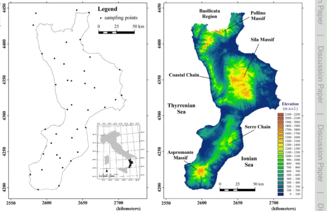
The study case was the Calabria region located in the southern part of the Italian peninsula (Fig. 1) with an area of 15 080 km2and a coastline of 738 km on the Ionian and Tyrrhenian seas. In the North, it borders Basilicata region for 80 km. Calabria has an oblong shape with a length of 248 km, and a width ranging between 31 and 111 km. 10
Although Calabria does not have many high summits, it is one of the most mountainous regions in Italy (Fig. 1): 42% of the land is mountainous, 49% hilly, and only 9% is flat. The maximum elevation is 2267 m a.s.l., while the average elevation is 597 m a.s.l.
Temperatures have been measured daily at 134 weather stations of the Italian Hy-drographic Service (at present “Centro Funzionale Multirischi della Calabria” of the 15
“Agenzia Regionale per la Protezione dell’Ambiente della Calabria” – Arpacal) dur-ing the period 1924–2009 (Fig. 1). Since it was focused on the month of June, only temperature data of this month were taken into account. Temperature time series hav-ing less than 30 years of observation were discarded and only temperature data from 42 weather stations were used. Some external stations were used to take into account 20
the border effect. To map June temperatures, a subset of elevation at points on a 250-m square grid fro250-m accurate digital elevation 250-model was used in si250-mulation as external drift variable.
The reference evapotranspiration was computed using the Hargreaves equation (Hargreaves and Samani, 1985), which can be expressed as:
25
ET0=0.0023Ra(T+17.8) q
HESSD
7, 4567–4589, 2010Uncertainty assessment in
modelling evapotranspiration
G. Buttafuoco et al.
Title Page
Abstract Introduction
Conclusions References
Tables Figures
◭ ◮
◭ ◮
Back Close
Full Screen / Esc
Printer-friendly Version Interactive Discussion
Discussion
P
a
per
|
Dis
cussion
P
a
per
|
Discussion
P
a
per
|
Discussio
n
P
a
per
where ET0 is the computed reference evapotranspiration (mm d− 1
); Ra is the water equivalent of the extraterrestrial radiation (mm d−1) computed according to Allen et al. (1998);Tmax,TminandT are the daily maximum, minimum and mean air temperature (◦C), withT calculated as the average ofT
maxandTmin. 0.0023 is the original empirical coefficient proposed by Hargreaves and Samani (1985). The monthly mean reference 5
evapotranspiration was obtained multiplying the result by 30 days.
Stochastic simulation of the input attributes
In this paragraph only a very brief introduction to the algorithm used in the case study will be given; for a detailed presentation, interested readers should refer to Goovaerts (1997), Chil `es and Delfiner (1999), among others. Most geostatistics is 10
based on the concept of a random functionZ(x), whereby the set of unknown values is regarded as a set of spatially dependent random variablesZ(xα). Each measure-ment of air temperature, z(xα), at different locationxα (x is the location coordinates vector andα the sampling points=1, ...,n) is interpreted as a particular realization of a random variableZ(xα).
15
Geostatistical simulation, compared with an optimal procedure of estimation such as kriging, provides a more realistic means of evaluating the spatial variability of a variable (Castrignan `o and Buttafuoco, 2004). Stochastic simulation results in a large number of equiprobable images, also called realizations, which honour the sample data and reproduce statistical characteristics and spatial features. Two types of simulations are 20
available using geostatistics: unconditional and conditional. Unconditional simulations simply reproduce certain statistical measures (mean, variance, covariance function) of a variable without considering the observed data. Conditional simulations generate realizations that incorporate the correlation structure of the data, honour the data and reproduce some random component of variation, which is smoothed out by kriging. 25
HESSD
7, 4567–4589, 2010Uncertainty assessment in
modelling evapotranspiration
G. Buttafuoco et al.
Title Page
Abstract Introduction
Conclusions References
Tables Figures
◭ ◮
◭ ◮
Back Close
Full Screen / Esc
Printer-friendly Version Interactive Discussion
Discussion
P
a
per
|
Dis
cussion
P
a
per
|
Discussion
P
a
per
|
Discussio
n
P
a
per
|
quality and computing time. This method was chosen because the weather stations having temperature data with more than 30 years of observations were sparse and few (only 42). Elevation is additional and denser information easily available, which can improve the estimation. In the scope of simulation with external drift, the variable of interestZ(x) comprises deterministic and stochastic components, then it can represent 5
the combination by the model:
Z(xα)=m(x)+ε(x) and E[Z(x)]=m(x). (2)
whereε(x) is the stochastic component with zero mean and variogramγε(h) andm(x) is the drift which is usually modelled as a linear function of a smoothly varying sec-ondary (external) variabley(x):
10
m(x)=a0(x)+a1(x)y(x). (3)
The principle is to simulate a target variable using an auxiliary linear correlated vari-able known at the grid nodes of the result grid file. The auxiliary correlated varivari-able in this case study was elevation because there is a good linear correlation between both June mean minimum (−0.90) and June mean maximum (−0.87) temperature data. The
15
value of the secondary variable (elevation) must be known at all primary data locations xα(α=1,...,n) and at all locationsx0being estimated. Moreover, the secondary vari-able should vary smoothly in space to avoid instability of the kriging with external drift system (Goovaerts, 1997). The simulation algorithm generates a 2-D simulation from the 1-D simulations along the lines. The turning bands method is a powerful and useful 20
mathematical operator (Christakos, 1987, 1992), however some authors (Deutsch and Journel, 1998) have criticised it because of the generation of artefacts in the simulated images. These artefacts are for the 3-D cases due to the limitation of a maximum of 15 lines which provide a regular partition of the 3-D space but there is no such limitation in 2-D. The turning band method consists in adding up a large number of independent 25
HESSD
7, 4567–4589, 2010Uncertainty assessment in
modelling evapotranspiration
G. Buttafuoco et al.
Title Page
Abstract Introduction
Conclusions References
Tables Figures
◭ ◮
◭ ◮
Back Close
Full Screen / Esc
Printer-friendly Version Interactive Discussion
Discussion
P
a
per
|
Dis
cussion
P
a
per
|
Discussion
P
a
per
|
Discussio
n
P
a
per
by a deconvolution process. The simulations along each line are discretized so that the same simulated value at a point is assigned to the “band” perpendicular to the line and containing the point. Hence, the name turning “bands” given to the method. The only parameter of this method is the count of bands that has been fixed to 400 in this work. This was a good compromise to save computer time and obtain good results. 5
Moreover, the number of realizations was fixed to 500 because high accuracies are reached only when the number of runs is sufficiently large.
The previous steps generate non-conditional realizations, which reproduce the given covariance function but do not honour the data. Conditioning is implemented in the software ISATIS®release 10.03 (www.geovariances.com) by kriging (Journel and Hui-10
jbregts, 1978; Chiles and Delfiner, 1999). The conditional simulation at locationx0is given by:
Zcs(x0)=Zs(x0)+ n X
L=1
λ0i[Z(xi)−Zs(xi)]. (4)
whereZcs(x0) is the conditional simulation at x0; Zs(x0) the non-conditional simula-tion at x0; z(xi) the experimental value at experimental location xi; Zs(xc) the non-15
conditional simulation at experimental locations xi; λ0i the kriging weight assigned at experimental locationxi when estimating at location x0; and n the number of exper-imental locations for kriging. As the turning bands method is a Gaussian simulation technique, it requires a multi-Gaussian framework. Therefore, each variable has ini-tially been transformed into a normal distribution with zero mean and unit variance, and 20
the simulation results have subsequently been back-transformed to the raw distribu-tion. Such procedure is known as Gaussian anamorphosis (Chil `es and Delfiner, 1999; Wackernagel, 2003), and it is a mathematical function which transforms a variable with a Gaussian distribution into a new variable with any distribution. The Gaussian anamorphosis can be achieved using an expansion into Hermite polynomials Hi(Y) 25
HESSD
7, 4567–4589, 2010Uncertainty assessment in
modelling evapotranspiration
G. Buttafuoco et al.
Title Page
Abstract Introduction
Conclusions References
Tables Figures
◭ ◮
◭ ◮
Back Close
Full Screen / Esc
Printer-friendly Version Interactive Discussion
Discussion
P
a
per
|
Dis
cussion
P
a
per
|
Discussion
P
a
per
|
Discussio
n
P
a
per
|
The joint turning bands simulation requires modelling and fitting a linear model of coregionalization (Goovaerts, 1997). The Linear Model of Coregionalization (LMC) is a quantitative measure of spatial correlation of the regionalized variablez(xi). It provides a method for modelling the direct and cross-variogram(s) of two or more variables so that the variance of any possible linear combination of these variables is positive. Any 5
experimental variogram is modelled as a combination of the same basic structures. The aim was to build a model which described the major spatial features of the attributes under study. The models used can represent bounded or unbounded varia-tion. In the former models, the variance (known as the sill variance) has a maximum at a finite lag distance (range) over which pairs of values are spatially correlated. In 10
this case, to model the coregionalization of the two attributes (Tmax and Tmin), three (N(N+1)/2) direct and cross variograms must be calculated and modelled jointly for the anamorphosed temperature data.
The best fitting function can be chosen by cross-validation, which checks the com-patibility between the data and the model. It takes each data point in turn, removing 15
it temporarily from the data set and using its neighbouring information to predict the value of the variable at its location. The estimate is compared with the measured value by calculating the experimental error, i.e. the difference between estimate and mea-surement, which can also be standardized by estimating the standard deviation. The goodness of fit was evaluated by the mean error (ME) and mean squared deviation 20
(MSDR). The mean error, which proves the unbiasedness of estimate if its value is close to 0, is given by:
ME=1
N N X
i=1 [z∗(x
i)−z(xi)]. (5)
whereN is the number of observation points, z∗
(xi) is the predicted value at location i, and z(xi) is the observed value at location i. The mean squared deviation ratio 25
HESSD
7, 4567–4589, 2010Uncertainty assessment in
modelling evapotranspiration
G. Buttafuoco et al.
Title Page
Abstract Introduction
Conclusions References
Tables Figures
◭ ◮
◭ ◮
Back Close
Full Screen / Esc
Printer-friendly Version Interactive Discussion
Discussion
P
a
per
|
Dis
cussion
P
a
per
|
Discussion
P
a
per
|
Discussio
n
P
a
per
is expressed as:
MSDR=1
N N X
i=1 [z∗(x
i)−z(xi)] 2
σ2(x i)
. (6)
If the model for the variogram is accurate, the mean squared error should equal the kriging variance and the MSDR value should be 1.
Then each geostatistical multivariate simulation has been used as input to the ET0 5
model. Probabilistic information has been extracted from the set of simulated images. By averaging the simulated values at each cell, two different maps have been pro-duced: the map of the expected value at any given location (E-type or Expected-value estimate; Journel, 1983) and the one of its standard deviation. The uncertainty in model predictions has been quantitatively evaluated from the replicate stochastic im-10
ages.
In sum, the proposed approach consisted in the following steps:
1. generating a set of input attributes (Tminand Tmax) realizationsai (i=1, . . . , 500) at nodes of a 250-m square grid using the joint stochastic simulation with elevation as external drift;
15
2. for this set of inputs realizations ai, computing the reference evapotranspiration using Eq. (1);
3. for each input and output attributes, computing average and standard deviation of the simulated values at each cell to produce the maps of the expected values at any given location and the ones of their standard deviation.
HESSD
7, 4567–4589, 2010Uncertainty assessment in
modelling evapotranspiration
G. Buttafuoco et al.
Title Page
Abstract Introduction
Conclusions References
Tables Figures
◭ ◮
◭ ◮
Back Close
Full Screen / Esc
Printer-friendly Version Interactive Discussion
Discussion
P
a
per
|
Dis
cussion
P
a
per
|
Discussion
P
a
per
|
Discussio
n
P
a
per
|
3 Results and discussion
The summary statistics of mean maximum (Tmax) and mean minimum temperature (Tmin) data (Celsius degrees) for June and elevation data (m a.s.l.). are reported in Ta-ble 1. The assumption of normal distribution was not accepted for both mean maximum (Tmax) and mean minimum temperature (Tmin) data at a probability levelp >0.10, and 5
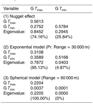
the data distributions showed long negative tails. Therefore, before conducting joint Gaussian simulation, we applied a Gaussian transformation toTmaxand Tmindata. No anisotropy was evident in the maps of the 2-D variograms (not shown) to a maximum lag distance of 100 km. A nested isotropic LMC (Table 2) was fitted to all the experi-mental direct and cross-variograms of the Gaussian transformed variables. The LMC 10
(Table 2) includes three different structures: a nugget effect, an exponential structure with a practical range of 30 000 m, and a spherical structure with a range of 60 000 m. The goodness of fit was evaluated by a cross-validation test and the results in terms of mean error (ME) and mean squared deviation (MSDR). ME ranged between−0.02
and−0.07, while MSDR between 0.92 and 0.93. The optimal values for the two
statis-15
tics are 0 for ME and 1 for MSDR, then the multivariate model of spatial correlation was unbiased and reproduced the experimental variance adequately. The sum of the eigenvalues at each spatial scale provides an estimate of the variance at that scale (Table 2). The nugget was about 50% of total variance (2.18), while the contribution of the shorter range component (30 000 m) of variation to the total variance was about 20
40% and the contribution of the longer range component (60 000 m) was 10%. The nugget effect component represents the unstructured spatial variation. It is mainly due to measurement errors and to the spatial variation at a scale lesser than the minimum distance of sampling. Moreover, in this study, the nugget ratio is due to the sparse and limited number of sampling locations. The variation at shorter scale (40%) is probably 25
HESSD
7, 4567–4589, 2010Uncertainty assessment in
modelling evapotranspiration
G. Buttafuoco et al.
Title Page
Abstract Introduction
Conclusions References
Tables Figures
◭ ◮
◭ ◮
Back Close
Full Screen / Esc
Printer-friendly Version Interactive Discussion
Discussion
P
a
per
|
Dis
cussion
P
a
per
|
Discussion
P
a
per
|
Discussio
n
P
a
per
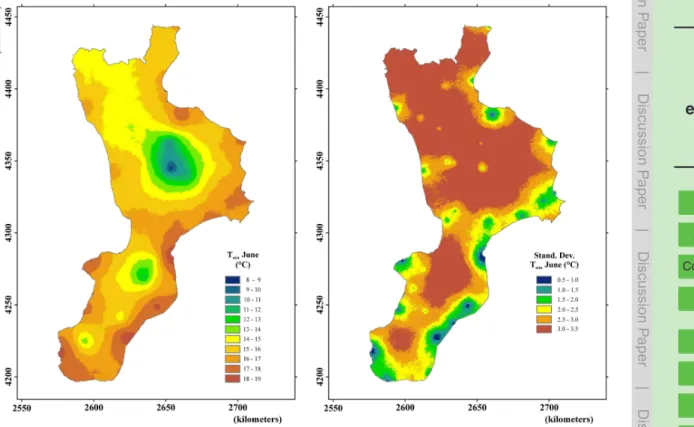
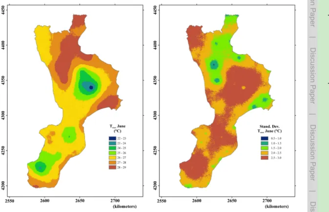
The above LMC was used to generate the 500 simulations ofTmin andTmaxat nodes of a 250-m square grid. Afterwards, the expected values of Tmin and Tmax and their standard deviation were computed and mapped: Fig. 2 and Fig. 3 present a way to treat the jointly simulated images of the two variables, by calculating the mean and the standard deviation respectively of the 500 simulations at each grid node, and then map-5
ping the results for each variable. The mean maps (Figs. 2 and 3) show the complexity in spatial distribution of temperatures. The maps of the standard deviation (Figs. 2 and 3), obtained by post-processing the simulations, have allowed to assess the uncertain-ties of non-Gaussian variables and to overcome the drawback of kriging variance of its independence from actual sample values. From a visual inspection, it shows clearly 10
how the uncertainty distributions of temperature are mostly related to the density of the sample data (Fig. 1). Figures 2 and 3 also show, as expected, that lower values of mean temperatures are estimated in correspondence to the mountainous areas (Sila Massif, Serre Chain and Aspromonte Massif) (Fig. 1), which have also the higher uncer-tainties (higher values of standard deviation). Figure 2 also shows a large area of the 15
region (the northern part) characterized by high values of standard deviation. These high values occurred in an area with high variability in elevation and consequently in temperature data at short distance.
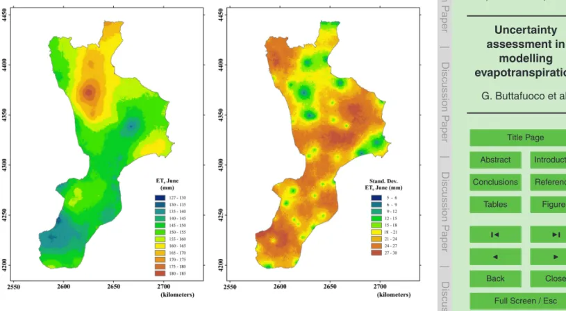
The 500 realizations of temperature data were used as input for ET0model and then the maps of the mean and standard deviation of ET0(Fig. 4) were obtained in a similar 20
way to the maps of Fig. 2 and Fig. 3. A visual inspection shows clearly where the uncertainty in ET0 is high. The simulation has shown how the previous uncertainties in input variables can affect the predictions of ET0model. In particular, one can note that there are extended areas characterised by high uncertainties localised on the Sila Massif, the Aspromonte Massif, the Serre Chain and the north-western portion of the 25
region. The areas characterised by medium-high values of ET0 present not very high values of standard deviation, and therefore less uncertainty.
HESSD
7, 4567–4589, 2010Uncertainty assessment in
modelling evapotranspiration
G. Buttafuoco et al.
Title Page
Abstract Introduction
Conclusions References
Tables Figures
◭ ◮
◭ ◮
Back Close
Full Screen / Esc
Printer-friendly Version Interactive Discussion
Discussion
P
a
per
|
Dis
cussion
P
a
per
|
Discussion
P
a
per
|
Discussio
n
P
a
per
|
is important to evaluate how well the model approximates reality, i.e. model uncertainty. If the model has high uncertainty, a difference in model output may not indicate a real change and could thus be meaningless.
4 Conclusions
The results of a spatial uncertainty analysis have shown that the prediction quality de-5
pends on the uncertainties of the data used in the analysis; therefore map makers should convey the accuracy of the maps they produce (Heuvelink, 1998). A complete characterisation of the accuracy of spatial data should also include the spatial correla-tion of the attributes used for estimacorrela-tion and stored in a GIS. In the past, a single root mean squared error was sufficient to assess spatial accuracy, but now it is no longer 10
sufficient, and much more information should be provided to characterise the quality of a map.
The objective of this study, however, was not to validate the model or assess the errors associated with the model type and coefficients, but rather to evaluate how the variability of inputs affects uncertainty of model prediction. By definition, a model is an 15
approximation of reality and some models describe reality better than others. There-fore, the choice of model plays an important role in error prediction. In this paper, however, it was assumed that an appropriate model was selected and that the model errors were associated only with the spatial variation of the input attributes.
In order to obtain realistic values of the model output uncertainty, when the model 20
outputs are supposed to be spatially correlated, it is critically important to model and assess spatial correlations of input variables (Heuvelink and Pebesma 1999). Ignoring spatial correlation between input variables, as in the traditional Monte Carlo approach, implies modelling input variables as white noise. In this case, all uncertainty in ET0 predictions might vanish after mapping with a dense point grid. The required density 25
HESSD
7, 4567–4589, 2010Uncertainty assessment in
modelling evapotranspiration
G. Buttafuoco et al.
Title Page
Abstract Introduction
Conclusions References
Tables Figures
◭ ◮
◭ ◮
Back Close
Full Screen / Esc
Printer-friendly Version Interactive Discussion
Discussion
P
a
per
|
Dis
cussion
P
a
per
|
Discussion
P
a
per
|
Discussio
n
P
a
per
are quite different. Spatial variation refers to the deterministic variation of ET0 or a single realization of the input attributes, whereas uncertainty refers to ET0distribution for a single point obtained from the ensemble of Monte Carlo simulations. The ap-proach would put more emphasis on the quality of the input data and on how the input uncertainties may have a considerable impact on prediction uncertainty. Looking at 5
the standard deviation map of ET0 (Fig. 4), only a weak spatial pattern can be distin-guished; the errors do not appear correlated with the estimates of ET0, but with the density of weather stations.
Finally, it is worth pointing out the consequences of estimation uncertainty in the context of decision-making and water resources management. There is currently some 10
reluctance to perform error recognition, possibly because of the greater analysis re-quired. However, studying uncertainty leads to increased understanding of the roles played by the different input attributes, which also allows to evaluate the relative costs and benefits of using different scenarios.
References
15
Allen, R. G., Pereira, L. S., Raes, D., and Smith, M.: Crop evapotranspiration – guidelines for computing crop water requirements, FAO Irrigation and Drainage, Paper no. 56, Rome, Italy, 1998.
Blaney, H. F. and Criddle, W. D.: Determining water requirements in irrigated area from clima-tological irrigation data. US Department of Agriculture, Soil Conservation Service, Techical
20
Paper no. 96, Washington, DC, USA, 1950.
Burrough, P. A.: GIS and geostatistics: Essential partners for spatial analysis, Environ. Ecol. Stat., 8, 361–377, 2001.
Castrignan `o, A. and Buttafuoco, G.: Geostatistical Stochastic Simulation of Soil Water Content in a Forested Area of South Italy, Biosyst. Eng., 87, 257–266, 2004.
25
Chil `es, J. P. and Delfiner, P.: Geostatistics: Modelling spatial uncertainty, Wiley, New York, USA, 1999.
HESSD
7, 4567–4589, 2010Uncertainty assessment in
modelling evapotranspiration
G. Buttafuoco et al.
Title Page
Abstract Introduction
Conclusions References
Tables Figures
◭ ◮
◭ ◮
Back Close
Full Screen / Esc
Printer-friendly Version Interactive Discussion
Discussion
P
a
per
|
Dis
cussion
P
a
per
|
Discussion
P
a
per
|
Discussio
n
P
a
per
|
Christakos, G.: Random field models in earth sciences, Academic Press, San Diego, CA, USA, 1992.
Deutsch, C. V. and Journel, A. G.: GSLIB: Geostatistical software library and user’s guide, Oxford University Press, New York, USA, 1998.
Droogers, P. and Allen, R. G.: Estimating reference evapotranspiration under inaccurate data
5
conditions, Irr. Drain. Syst., 16, 33–45, 2002.
Dyck, S.: Overview on the present status of the concepts of water balance models, in: Proceed-ing of the Hamburg Workshop New Approaches in Water Balance Computations, Hamburg, 15–29 August 1983, IAHS Publication no. 148, 3–19, 1983.
Gomez-Hernandez, J. J. and Journel, A. G.: Joint sequential simulation of multigaussian fields,
10
in Geostat Troia 1992, Kluwer Publ. Dordrecht, Holland, 1992.
Gong, L., Xu, C. Y., Chen, D., Halldin, S., and Chen, Y. D.: Sensitivity of the Penman–Monteith reference evapotranspiration to key climatic variables in the Changjiang (Yangtze River) basin, J. Hydrol., 329, 620–629, 2006.
Goovaerts, P.: Geostatistics for Natural Resources Evaluation, Oxford University Press, New
15
York, USA, 1997.
Hargreaves, G. H. and Samani, Z. A: Reference crop evapotranspiration from temperature, Appl. Eng. Agric., 1, 96–99, 1985.
Hargreaves, G. H. and Allen, R. G.: History and evaluation of Hargreaves evapotranspiration equation, J. Irrig. Drain. E-ASCE, 129, 53–63, 2003.
20
Hargreaves, G. L., Hargreaves, G. H., and Riley, J. P.: Agricultural benefits for Senegal River basin, J. Irrig. Drain. E-ASCE, 111, 113–124, 1985.
Heuvelink, G. B. M.: Error propagation in environmental modeling with GIS, Taylor, Francis, London, UK, 1998.
Heuvelink, G. B. M. and Pebesma, E. J.: Spatial aggregation and soil process modelling,
Geo-25
derma, 89, 47–65, 1999.
Hobbins, M. T., Ramirez, J. A., and Brown, T. C.: The complementary relationship in estimation of regional evapotranspiration: an enhanced advection-aridity model, Water Resour. Res., 37, 1389–1403, 2001a.
Hobbins, M. T., Ramirez, J. A., Brown, T. C., and Claessens, L. H. J. M.: The
complemen-30
HESSD
7, 4567–4589, 2010Uncertainty assessment in
modelling evapotranspiration
G. Buttafuoco et al.
Title Page
Abstract Introduction
Conclusions References
Tables Figures
◭ ◮
◭ ◮
Back Close
Full Screen / Esc
Printer-friendly Version Interactive Discussion
Discussion
P
a
per
|
Dis
cussion
P
a
per
|
Discussion
P
a
per
|
Discussio
n
P
a
per
Hudson, G. and Wackernagel, H.: Mapping temperature using kriging with external drift: theory and an example from Scotland, Int. J. Climatol., 14, 77–91, 1994.
Jensen, M. E.: Consumptive use of water and irrigation water requirements, American Society of Civil Engineers, New York, USA, 1973.
Journel, A. G. and Huijbregts, C. J.: Mining Geostatistics, Academic Press, New York, USA,
5
1978.
Journel, A. G.: Non-parametric estimation of spatial distributions, Math. Geol., 15, 445–468, 1983.
Penman, H. L.: Natural evaporation from open water, bare soil and grass, P. Roy. Soc. Lond. A. Mat., 193, 120–145, 1948.
10
Wackernagel, H.: Multivariate Geostatistics: an introduction with applications, Springer-Verlag, Berlin, Germany, 2003.
Xu, Z. X. and Li, J. Y.: A distributed approach for estimating catchment evapotranspiration: comparison of the combination equation and the complementary relationship approaches, Hydrol. Process., 17, 1509–1523, 2003.
15
Xu, C. Y. and Singh, V. P.: Cross-comparison of empirical equations for calculating potential evapotranspiration with data from Switzerland, Water Resour. Manag., 16, 197–219, 2002. Xu, C. Y. and Singh, V. P.: Evaluation of three complementary relationship evapotranspiration
models by water balance approach to estimate actual regional evapotranspiration in different climatic regions, J. Hydrol., 308, 105–121, 2005.
HESSD
7, 4567–4589, 2010Uncertainty assessment in
modelling evapotranspiration
G. Buttafuoco et al.
Title Page
Abstract Introduction
Conclusions References
Tables Figures
◭ ◮
◭ ◮
Back Close
Full Screen / Esc
Printer-friendly Version Interactive Discussion
Discussion
P
a
per
|
Dis
cussion
P
a
per
|
Discussion
P
a
per
|
Discussio
n
P
a
per
|
Table 1. Basic statistics of mean maximum (Tmax) and mean minimum temperature (Tmin) data
(Celsius degrees) for June and elevation data (m a.s.l.).
HESSD
7, 4567–4589, 2010Uncertainty assessment in
modelling evapotranspiration
G. Buttafuoco et al.
Title Page
Abstract Introduction
Conclusions References
Tables Figures
◭ ◮
◭ ◮
Back Close
Full Screen / Esc
Printer-friendly Version Interactive Discussion
Discussion
P
a
per
|
Dis
cussion
P
a
per
|
Discussion
P
a
per
|
Discussio
n
P
a
per
Table 2. Fitted linear model of coregionalization of anamorphosedTmax (GTmax) and Tmin (G
Tmin). The coregionalization matrices, the eigenvalues, and the corresponding percentage of variance explained by each eigenvector for the three basic structures are reported.
Variable GTmax GTmin
(1) Nugget effect GTmax 0.5613
GTmin 0.2752 0.5784 Eigenvalue: 0.8452 0.2945
(74.16%) (25.84%)
(2) Exponential model (Pr. Range=30 000 m) GTmax 0.3108
GTmin 0.3589 0.5168
Eigenvalue: 0.7872 0.0403 (95.13%) (4.87%) (3) Spherical model (Range=60 000 m) GTmax 0.2204
GTmin 0.0037 0.0001 Eigenvalue: 0.2205 0.0000
HESSD
7, 4567–4589, 2010Uncertainty assessment in
modelling evapotranspiration
G. Buttafuoco et al.
Title Page
Abstract Introduction
Conclusions References
Tables Figures
◭ ◮
◭ ◮
Back Close
Full Screen / Esc
Printer-friendly Version Interactive Discussion
Discussion
P
a
per
|
Dis
cussion
P
a
per
|
Discussion
P
a
per
|
Discussio
n
P
a
per
|
HESSD
7, 4567–4589, 2010Uncertainty assessment in
modelling evapotranspiration
G. Buttafuoco et al.
Title Page
Abstract Introduction
Conclusions References
Tables Figures
◭ ◮
◭ ◮
Back Close
Full Screen / Esc
Printer-friendly Version Interactive Discussion
Discussion
P
a
per
|
Dis
cussion
P
a
per
|
Discussion
P
a
per
|
Discussio
n
P
a
per
|
HESSD
7, 4567–4589, 2010Uncertainty assessment in
modelling evapotranspiration
G. Buttafuoco et al.
Title Page
Abstract Introduction
Conclusions References
Tables Figures
◭ ◮
◭ ◮
Back Close
Full Screen / Esc
Printer-friendly Version Interactive Discussion
Discussion
P
a
per
|
Dis
cussion
P
a
per
|
Discussion
P
a
per
|
Discussio
n
P
a
per