http://dx.doi.org/10.1590/S1982-21702014000200020
ON ACCURATE GEOID MODELING: DERIVATION OF
DIRICHLET PROBLEMS THAT GOVERN GEOIDAL
UNDULATIONS AND GEOID MODELING BY MEANS OF
THE FINITE DIFFERENCE METHOD AND A HYBRID
METHOD
Sobre modelagem acurada do geóide: Derivação de Problemas de Dirichlet que governam ondulações geoidais e modelagem do geóide pelo Método das Diferenças
Finitas e um Método Híbrido
EDUARDO DEL RIO
Kyoto University, Graduate School of Science, Department of Geophysics, Geodesy Laboratory, Kyoto, Japan
Instituto Militar de Engenharia, Programa de Pós-graduação em Engenharia de Defesa, Laboratório de Posicionamento, Rio de Janeiro, Brazil
ABSTRACT
optimal combination of techniques by means of a Hybrid method and shown that it alleviates the uncertainty in Finite Difference Method. Moreover, a rigorous error analysis indicates that the Hybrid method proposed here may well outperform Stokes's Integral.
Keywords: Geoid Modeling; Ellipsoidal Dirichlet Problem; Finite Difference Method; Stokes's Integral.
RESUMO
O geóide é a superfície de referência utilizada para se medire altitudes (ortométrica). Estas são utilizadas para estudar qualquer variação de massa no sistema terrestre. Como a Terra é representada por um esferóide oblatado (elipsóide), o geóide é determinado por meio de ondulações geoidais (N) que são a separação entre essas superfícies. N é determinado a partir de dados gravitacionais pela integral de Stokes. Todavia, esta abordagem considera uma Terra esférica ao invés de elipsóidica. Neste artigo é deduzida uma equação diferencial parcial (sigla em inglês PDE) que governa N ao redor da Terra por vias de um Problema de Dirichlet. Também mostra-se aqui um método para resolver esta PDE que dispensa a necessidade de uma Terra esférica. Além do mais, a Integral de Stokes resolve um problema de valor de contorno definido por toda a Terra. Descobriu-se que o Problema de Dirichlet aqui proposto está definido apenas ao longo da região de cálculo o que é vantajoso para modelamento local do geóide. Além do mais, o método elimina diversas das fontes de incertezas presentes na Integral de Stokes. Todavia, estimativas indicam que o erro devido à discretização é muito grande neste novo método o que pede por modificações. Sendo assim, aqui também propõe-se uma combinação ótima de técnicas por meio de um método Híbrido. Mostra-se que que este método híbrido atenua as incertezas do método das Diferenças Finitas. Além do mais, uma rigorosa análise de erros indica que o método Híbrido aqui proposto pode bem desempenhar melhor do que a Integral de Stokes.
Palavras-chave: Modelagem do Geóide; Problema de Dirichlet no Elipsóide; Método das Diferenças Finitas; Integral de Stokes.
1. INTRODUCTION
quality as for geodesists (SANSO and SIDERIS, 2013; TAPLEY et al., 2004) which is hardly attainable without methods of improved accuracy. However, the ellipsoidal corrections do not eliminate the error from the spherical approximation but attenuate it. Moreover, they still have the following errors: limiting the area of integration to a small spherical cap (truncation error), approximating the normal derivative by a radial or other derivative, Earth's topography that cause to exist masses outside the geoid, discretization of the input gravity and propagation of the uncertainties of the input gravity.
The Boundary Value Problem (BVP) from which Stokes’s Integral is derived is defined over the whole space on and outside the geoid and over the whole geoid. Consequently, its solution requires gravity data over the whole Earth to provide N at a single point. The Dirichlet problem derived here is defined only over the region of computation. Thus, besides computing N directly on the ellipsoid, its solution requires gravity data only over the region of interest. In solving a Dirichlet problem in the Ellipsoid these 3 major sources of error will be eliminated: the spherical approximation, the truncation of the integral and the Earth's topography.
A Dirichlet problem whose PDE governs N over the geoid is derived here and it is shown how to numerically solve it by using the Finite Difference Method (FDM). However this method can handle considerably large matrices which increases its computational cost. Therefore, it is also proposed a modification on FDM (FDM with subgrids, FDM2) that allows the computation of geoid models of large regions by keeping the matrices involved at a small and constant size. It will be shown here that FDM has large errors due to discretization so it is also proposed a Hybrid method to alleviate those uncertainties. To derive it it will be needed a Spherical Dirichlet Problem which will also be derived here. The Hybrid method as opposed to FDM yields subcentimetric differences from Stokes's Integral. Moreover, an error analysis will be developed which indicates that the Hybrid method may well outperform Stokes's Integral.
2. DERIVATIONS OF STOKES’S INTEGRAL AND DIRICHLET PROBLEM
Stokes’s Integral is derived from the fundamental Equation of Physical Geodesy (HOFMANN-WELLENHOF et al., 2006):
Stokes’s Integral makes a spherical approximation on Eq. (1) to then compute an integral solution for the BVP considering the whole space outside the geoid. To derive the Dirichlet problem for FDM it is considered the generalized Poisson’s Equation in ellipsoidal-harmonic coordinates (u, υ, λ) for the gravitational and the normal potentials to derive the Laplacian of T, which inside the Earth is as follows (SANSO and SIDERIS, 2013) (υ is the complement of the reduced latitude β, i.e. β
= π/2 − υ , and λ is the geocentric longitude):
where u is lesser than or equals b, E=(a2−b2)1/2 is the linear eccentricity, with a being the semi-major axis and b the semi-minor axis of the Ellipsoid of revolution, G is the gravitational constant and ρ is the Earth’s density.
2.1 The Dirichlet Problem PDE
The PDE that describes T over the Earth, and thus, solely as a function of T and its partial derivatives in υ and λ can be derived from Eqs. (1) and (3) after expressing Eq. (1) in ellipsoidal-harmonic coordinates u, υ and λ, for details refer to Appendix A. This PDE is as follows:
where BN(υ), CN(υ), FN(υ), GN(υ, λ) are as follows:
This PDE together with its boundary condition, which is to know T or N (geoidal undulation) at the boundary of the surface where it’s been applied, defines an Elliptic BVP with a Dirichlet boundary condition. This, in turn, defines a Dirichlet problem, which can be solved numerically by e.g. FDM.
3. NUMERICAL SOLUTION OF THE DIRICHLET PROBLEM BY FDM AND FDM2
To obtain T by FDM the partial derivatives of T must be expressed by their equivalent form in finite differences (DIEGUEZ, 2005). In other words, to make the following substitutions—considering data on a grid (j, i), 1<j<J−1 and 1< i< I−1:
where ∆λ and ∆υ are the grid spacing.
Substituting Eqs. (9), (10) and (11) in Eq. (4) yields the final expression for FDM:
where BN, CN, FN and GN are given by Eqs. (5), (6), (7) and (8).
linear system on more than 57 thousand variables which in double precision requires more than 24.3 Gigabytes of Random Acess Memory (RAM). This can be big for a personal computer to handle. Therefore it is proposed a Finite Difference Method with subgrids (FDM2) to compute geoid models of regions as big as desired while keeping the linear system as small as desired. FDM2 is best suited for high resolution geoid modeling. For further details on FDM2 refer to Fig. 1.
3.1 Short Remark on Remove-Compute-Restore Technique and FDM
In FDM, terrain reductions are not mandatory because the Dirichlet problem is derived from Poisson's equation as opposed to Stokes's Integral. Moreover for FDM and FDM2 the long wavelengths need not be removed because the Dirichlet problem is defined only over the region of computation as opposed to the BVP from which Stokes's Integral is derived which is defined over the whole Earth. Therefore, FDM does not require implementation of a remove-compute-restore technique.
Figure 1 – How FDM2 works. The grid (big square) is divided in subgrids (small squares, as many as desired, here 16 for the sake of simplicity). FDM is applied individually to each subgrid instead of a single run on the grid. In addition, T or N
Figure 2 - Region used for assessment of geoid modeling methods. The region where the geoid models were computed is represented by the solid black square.
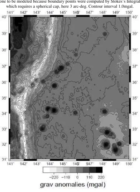
Figure 3 - Input gravity anomalies used.The input data spans a larger area than the one to be modeled because boundary points were computed by Stokes’s Integral
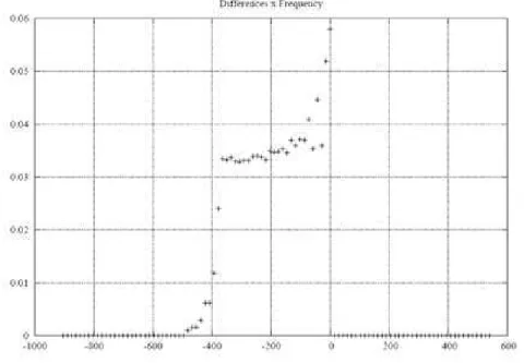
Figure 6 - Histogram of differences between FDM and Stokes’s Integral (cm). The frequency is represented by means of probability, i.e. their sum equals 1.
Table 1 - Differences between FDM and Stokes's Integral. Max, min, mean and sd are the maximum, the minimum, the mean and the standard deviation of the
differences between the techniques. Values are in cm.
Resolution Max Min Mean sd
1 arc-deg 0.0 -96.7 -69.0 132.2
1 arc-min 0.0 -492.0 -189.7 121.6
The differences between FDM and Stokes's Integral are displayed in Table 1 for the 1deg and the 1min grids. It can be observed that an increase in resolution improves the quality of the grid as given by the standard deviation (sd). In both grids, the differences were very large, much greater than the decimeter. However, it is known that the sd of Stokes's Integral over Japanese lands is subdecimetric as measured by Kuroishi (2009) and Odera et al. (2012). Thus, this large deviation is mainly due to the errors of discretization of input and propagation of input uncertainties in FDM, see Eq. (A.5), Appendix B.
Importantly, for the 1min grid the computation of such grid for N was not possible by FDM due to the large number of variables but only by FDM2 (FDM2 was designed for the case when FDM cannot be applied). FDM2 was applied with squared subgrids sizing 1deg. In total, 9 subgrids were required. The 1deg grid has too few points to yield a reasonable implementation of FDM2. Therefore, the 1deg grid was computed only by FDM and the 1min grid was computed only by FDM2.
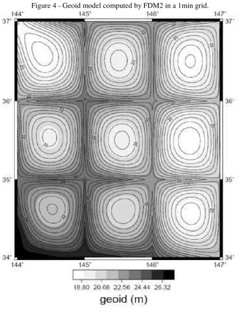
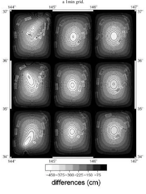
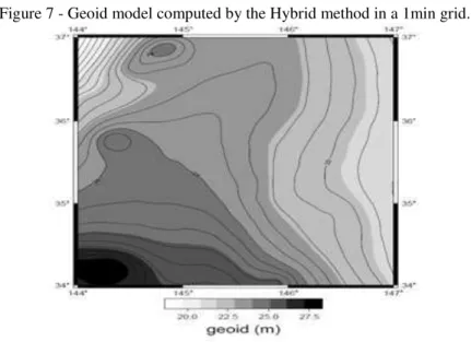
The map of the grid concerning the input gravity anomalies is displayed on Fig. 3. The geoid model computed in a 1min grid using FDM2 is displayed on Fig. 4. The map of the differences between FDM2 and Stokes’s Integral in the 1min grid corresponds to Fig. 5. In the difference map it can be observed significant deviations between the methods. The deviation is null at the boundary of each subgrid and generally increases towards their center. Moreover, a plot of the histogram of the differences is displayed on Fig. 6. As given by a -1.2 kurtosis, it indicates that the differences conform to a uniform distribution.
To alleviate the large uncertainties in FDM it will be proposed here a Hybrid Method. Prior to its formulation it is necessary to derive a Spherical Dirichlet problem.
5. DERIVATION OF A SPHERICAL DIRICHLET PROBLEM
Considering Poisson's equation in spherical coordinates and the fundamental equation of physical geodesy in spherical approximation it can be derived a Spherical Dirichlet problem that will be used to alleviate the uncertainties in the Ellipsoidal Dirichlet problem. The equations read as follows:
where BN(υ), CN(υ), FN(υ), GN(υ , λ) are as follows:
for the Earth 4πGρ is very small and can be neglected.
Its finite difference expression is similar to that of the Ellipsoidal Dirichlet problem and reads:
where BN(υ), CN(υ), FN(υ), GN(υ, λ) are given by Eqs. (16), (17), (18) and (19).
6. THE UNCERTAINTIES INVOLVED IN EACH TECHNIQUE FOR GEOID MODELING
Here it will be derived expressions that give the true N at a point as N computed by a technique plus uncertainties due to each error source. In symbols, denoting the N computed from an Ellipsoidal Dirichlet problem by NFDME, from a Spherical Dirichlet problem by NFDMS and from the remove-compute-restore (RCR) technique by NRCR it follows:
error due to the topographical masses outside the geoid and εT is the error due to truncation of Stokes’s Integral. εTopo and εT are alleviated because of the implementation of RCR technique. εE and ε1 are considered equal or very similar for both NRCR and NFDMS because the same approximation is done in both cases.
7. ALLEVIATION OF THE UNCERTAINTIES IN FDM BY AN OPTIMAL COMBINATION OF TECHNIQUES
The uncertainty due to discretization of input and propagation of input uncertainties can be alleviated if N is computed by the following formula:
Note that Eq. (22) gives N as a combination from N computed by several techniques. This optimal combination shifts the error due to discretization to that of Stokes’s Integral, which is much smaller. Moreover, εT , εTopo and ε′1 are small, with
εT and εTopo being alleviated by RCR’s implementation and the same being possible for ε′1 in future. So, the error of this new method is mainly due to discretization of input and propagation of the uncertainties of the input in Stokes’s Integral, which are much smaller compared to FDM. Hereafter, I will refer to the N given by this method as NHybrid, i.e.
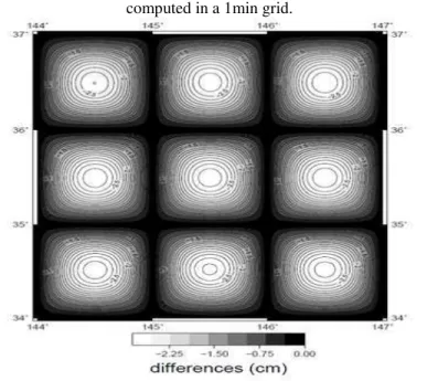
Figure 8 - Map of the differences between the Hybrid method and Stokes’s Integral computed in a 1min grid.
Table 2 - Differences between the Hybrid Method and Stokes's Integral. Max, min, mean and sd are the maximum, the minimum, the mean and the standard deviation
of the differences between the techniques. Values are in cm.
Resolution Max Min Mean sd
1 arc-min 0.0 -2.86 -1.30 0.83
8. COMPARISON OF THE HYBRID METHOD WITH STOKES’S INTEGRAL
It was computed N in a 1min grid over 34o − 37oN and 144o − 147oE using the same input grid of gravity anomalies. In this region NHybrid and the difference NHybrid − NRCR were computed. The differences are dislayed on Table 2. Kurtosis is -1.20 which indicates that the differences again conform to a uniform distribution. Moreover, the difference may be expressed as follows:
so that the difference is a measure of the uncertainty due to the Earth’s ellipticity that is usually not accounted for in RCR. From Eqs. (9) and (10) NHybrid’s uncertainty is expected to be inferior to that of NRCR as ε1 and ε′1 may be considered as approximately equal. NHybrid has the advantage over Stokes’s Integral of eliminating εE and possibly eliminating ε′1 in future. The maximum observed difference is very small in magnitude and σ is below centimeter which is remarkable. Moreover, the differences were again null at the boundary of each subgrid and tended to increase towards their center. The same trend was observed here for the Hybrid method. The geoid computed by the Hybrid method is displayed on Fig. 7 and represents the geoid over the region much more accurately than the sole FDM. The difference map is displayed on Fig. 8. The histogram of the differences is displayed on Fig. 9.
9. CONCLUSIONS AND FUTURE WORK
In this article the formulations of a Dirichlet problem to compute geoidal undulations and its numerical solution by FDM were proposed. The main advantages are the elimination of the errors due to the neglection of Earth's flattening, truncation of Stokes's Integral and the Earth's topography. The major drawback of this approach is the error due to the limited density of the input gravity. Moreover, an optimal combination of techniques was proposed here and named Hybrid method.
However, FDM and FDM2 are not as yet alternatives for highly accurate geoid determinations in this time when a 1cm geoid is desired. This is mainly due to the error due to discretization of input and the propagation of uncertainties in the input which were shown to be much larger in FDM and FDM2 than in Stokes's Integral. Therefore, future work should concern with the treatment of such uncertainties in order to make FDM and FDM2 comparable or even better than Stokes's Integral just in the way that was done here by means of the Hybrid method. Afer all, an increase in resolution decreased the uncertainty of FDM, so it is expected that in future, with more gravity data of higher quality and denser coverage available, the overall uncertainty of FDM will decrease. Moreover, FDM and FDM2 eliminate 3 major sources of uncertainty in Stokes's Integral.
The error analysis was derived here and it was found that the uncertainty in the Hybrid method is mainly due to the discretization of input and propagation of input uncertainties in Stokes's Integral because other uncertainties cancel each other or are comparably small. This led to very small uncertainties and a remarkable agreement with Stokes's Integral as opposed to FDM.
The differences between the Hybrid method and Stokes's Integral are due to the Earth's ellipticity so that it is expected that the use of ellipsoidal corrections in future work may further improve NRCR and consequentely NHybrid as well. Moreover, these differences show that for a centimetric geoid a Spherical Earth should not be used.
Further suggestions for future work: if the required data is available, it would be good to compute a geoid model in land in order to compare results with geoidal undulations determined by spirit levelling. Also good would be to compare FDM/FDM2 with Stokes's Integral on ellipsoidal correction in order to improve accuracy of boundary points and slightly improve overall accuracy of geoid model. To derive a PDE for the Dirichlet problem based on a more accurate approximation of the vertical gradient of T, e.g. using the normal to the Ellipsoid, is the final suggestion for future work.
Furthermore, once the error due to the Earth's ellipticity is similar for NRCR and NFDMS techniques, from the error analysis developed here it is expected that the Hybrid method will outperform Stokes's Integral which would be a step towards a centimetric geoid.
ACKNOWLEDGEMENTS:
I would like to thank Prof. Yoichi Fukuda for careful review of the paper and perceptive points.
REFERENCES
ANDERSEN O.B. The DTU10 Gravity field and Mean sea surface. Second international symposium of the gravity field of the Earth (IGFS2), Fairbanks, Alaska, 2010.
ARDESTANI V.; MARTINEC Z. Geoid Determination Through Ellipsoidal Stokes Boundary-value Problem by Splitting its Solution to the Low-degree and the High-degree Parts. Studia geoph. et geod. v. 41, p. 73-82, 2003.
DEL RIO E. fdiff1 - FORTRAN90 software to compute geoid models by FDM and Stokes’s Integral. 2013. Available at mendeley.com/profiles/eduardo-del-rio DEL RIO E. fdiff2 - FORTRAN90 software to compute geoid models by FDM2 and
Stokes’s Integral. 2013. Available at mendeley.com/profiles/eduardo-del-rio DIEGUEZ J.P.P. Métodos de Cálculo Numérico. Fundação Ricardo Franco, 2005.
In Portuguese language.
HIPKIN H.G. Ellipsoidal geoid computation. J. Geod. v. 78, p. 167-179, 2004. HOFMANN-WELLEHOF B.; MORITZ H. Physical Geodesy. Springer Wien
NewYork, Germany, Second edition, 2006.
KUROISHI Y. Improved geoid model determination for Japan from GRACE and a regional gravity field model. Earth Planets Space v. 61, p. 807-813, 2009. MARTINEC Z.; GRAFAREND E.W. Solution to the Stokes Boundary-value
problem on an Ellipsoid of Revolution. Studia geoph. et geod. v. 41, p. 103-129, 1997.
NAJAFI-ALAMDARI M.; EMADI S.R.; MOGHTASED-AZAR K. The ellipsoidal correction to the Stokes kernel for precise geoid determination. J. Geod. v. 80, p. 675-689, 2006.
ODERA P.A.; FUKUDA Y.; KUROISHI Y. A high-resolution gravimetric geoid model for Japan from EGM2008 and local gravity data. Earth Planets Space v. 64, p. 361-368, 2012.
PAIL R.; BRUINSMA S; et al. First GOCE gravity field models derived by three different approaches. J. Geod. v. 85, p. 819-843, 2011.
PAIL R.; GOIGINGER W.; et al. Combined satellite gravity field model GOCO01S derived from GOCE and GRACE. Geophys. Res. Lett. v. 37, L20314, 2010. PAVLIS N.K.; HOLMES S.; KENYON S.C.; FACTOR J.K. The development and
evaluation of the Earth Gravitational Model 2008 (EGM2008). J. Geophys. Res. v. 117, B04406, 2012.
SANSO F.; SIDERIS M. Geoid Determination Theory and Methods. Springer, Germany, 2013.
TAPLEY B.; BETTADPUR S.; et al. GRACE measurements of mass variability in the Earth system. Science v. 305, p. 503-50, 2004.
APPENDIX A – DETAILS ON THE DERIVATION OF DIRICHLET PROBLEM PDE
To express Eq. (1) in ellipsoidal-harmonic coordinates, the vertical gradient of T will be approximated by its derivative with respect to u as follows
where ∂T/∂n denotes the normal derivative measured along the outward unit normal to the ellipsoid.
Hence,
where F(υ) is given by:
where M = a2/ [b(1+e′2cos2υ)3/2] and N = a2/ [b(1+e′2cos2υ)1/2]. In M and N (these are the radius of curvature in the direction of the meridian and the normal radius of curvature in the direction of the prime vertical), υ is the ellipsoidal latitude and e′ is the second eccentricity, where e′ = (a2−b2)1/2/b.
Consequently, by derivating Eq. (A.1) with respect to u yields:
where ∂∆g/∂u is approximated by the vertical gradient of the gravity anomaly
∂∆g/∂h or its radial derivative with respect to the Earth’s center of mass. The PDE for the Dirichlet problem is obtained by substituting the first and second derivatives of T with respect to u from Eqs. (A.1) and (A.3) in Eq. (3).
APPENDIX B – THE ERROR INTRINSIC TO STOKES’S INTEGRAL A major source of error that is present in geoid modeling is the discretization of the input and the propagation of the input errors. It is considered that the error due to discretization/propagation is approximately equal for all techniques. Thus, letting N be the true geoidal undulation and N′ be the computed geoidal undulation yields:
where ε0 is the error due to approximation of the normal derivative of T by ∂T/∂u,
Letting ∆N = NFDM−NStokes with NStokes=NFDM implies:
Thus, by comparison with FDM/FDM2 the uncertainty in due to discretization/propagation can be estimated fairly according to Eq. (A.5) because ε′0 − ε0 is small compared to the other terms.