A REVIEW OF INTELLIGENT CONTROL SYSTEMS APPLIED TO THE INVERTED-PENDULUM PROBLEM

(1)

American Journal of Engineering and Applied Sciences 7 (2): 194-240, 2014 ISSN: 1941-7020

doi:10.3844/ajeassp.2014.194.240 Published Online 7 (2) 2014 (http://www.thescipub.com/ajeas.toc)

Corresponding Author: Pedro Ponce, Department of Engineering, Tecnologico de Monterrey, Mexico City, Mexico

A REVIEW OF INTELLIGENT CONTROL SYSTEMS

APPLIED TO THE INVERTED-PENDULUM PROBLEM

Pedro Ponce, Arturo Molina and Eugenio Alvarez

Department of Engineering, Tecnologico de Monterrey, Mexico City, Mexico

Received 2014-03-08; Revised 2014-03-14; Accepted 2014-04-07

ABSTRACT

This study shows the latest advances in the application of intelligent control to the inverted-pendulum problem. A complete review regarding intelligent control design is presented in this study in order to show the most important artificial intelligence methods used for controlling an Inverted-Pendulum. Also this study proposed the use of a neural-fuzzy-with-genetic-algorithms controller for the inverted pendulum problem which gives good results. Conventional controllers are presented in order to observe implementation problems. The study goes deeply in the details that have to take into account in order to understand design problems and limitations.

Keywords: Inverted Pendulum, Intelligent Control, Fuzzy Logic, Neural Networks, Genetic Algorithms, ANFIS, Unstable Nonlinear Systems

1. INTRODUCTION

The inverted pendulum is a classical example of an instable, nonlinear system that has been solved in many ways but remain a prototypical case study for optimization and the testing of new control techniques. The inverted pendulum system is made of a rigid rod and a car to which the rod is joined by a bolt providing it with rotational freedom. The bar involves a frictionless union with one degree of freedom. The car can move rightwards or leftwards over tracks according to the force exerted upon it. The control objective is to keep the bar on balance, beginning from nonzero initial conditions, in such a way that the bar remains oriented upwards despite possible perturbations and the system’s intrinsic unstability (Jang, 1992; Lundeberg, 1994; Williams and Matsuoka, 1991; Jacobs and Jordan, 1993; Kitamulra and Saitoh, 1990; Kouda et al., 2002; Sazonov et al., 2003; Mohanlal and Kaimal, 2002; Inoue et al., 2002; Harrison, 2003; Chen and Chen, 2003; Pal and Pal, 2003; Lam et al., 2003; Cho and Jung, 2003; Gao and Er, 2003; Olguín, 2000; Jang, 1992; Ji et al., 1997; DECE, 2003; Omatu and Ide, 1994; Ravn and Poulsen, 2001; Jang-Sun-Mizutani, 1997; Riedmiller, 1993; Omatu et al., 2000; Jang, 1993;

Nørgaard, 2000a; 2000b; Omatu et al., 1995; Storn and Price, 1997; Mirza and Hussain, 2000; Messner and Tilbury, 1999; Bishop and Dorf, 1999; Takagi and Sugeno, 1985; Olguín, 2003; Yang et al., 2000; Jung and Yim, 2000). This dynamical system can be characterized by four state variables, namely Equation 1:

(

)

T

s

x = θ θ x x (1)

Where:

θ = The angle that the bar makes with the vertical (or horizontal) axis

θ = The angular speed of the bar

x = The position of the car relative to the tracks and x = The linear speed of the car

As mentioned before, the control objective is to set the car in its central position (x = 0) in such a way that the pendulum remains in its vertical position, with its bob pointing upwards.

For our purposes, this means Equation 2:

x x 0

(2)

Fig. 1. Schematics of the inverted pendulum system Table 1. Parameters for the simulated inverted pendulum

M Mass of the car 0.455 kg

m Mass of the pendulum 0.21 kg

l Distance from the 0.305 m

pendulum’s center of mass

I Moment of inertia of the pendulum 0.006 kg*m2

Fig. 1 shows the system that is assumed for this project. The parameters used in the simulation are used in Table 1.

The inverted pendulum has a great importance for its application in practical systems. In the military arena, it provides a framework for understanding the remote control of rockets, as they undergo sizable perturbations at launching due to fuel explosion that make it necessary to guarantee the desired orientation. There has been considerable work in other aero-spatial applications as well. The inverted pendulum is also a relevant model for understanding the way in which structures with two feet (such as human being and some robots) may walk while keeping balance (Lundeberg, 1994). Several solutions to the inverted-pendulum problem are known, so that research has increasingly emphasized the more complex cases of pendulum with two, three or more bars, as well as deformable pendulum (non-rigid bars) and multidimensional pendulum. These systems have more inputs and outputs in need of control, which makes them rather more unstable and nonlinear.

The control law based on a conventional PID control is quite complex for one-input, two-output (SIMO) systems, such as the inverted pendulum case. Because of that, modern control theories are generally used in the

control design of these systems. These techniques include state feedback, adaptive-control strategies, neural-network modeling to simulate possible combinations of input/output control, adaptive or intelligent neural-network controllers and, more recently, the integrated application of neural networks and fuzzy-logic. This is so because fuzzy control requires an expert control law for the inverted pendulum formulated in terms of if-then rules. A recently designed controller, described in an IEEE publication, uses genetic algorithms, neural networks and fuzzy logic to tune a PID controller. Many neural-network architectures have proposed to control an inverted pendulum (Williams and Matsuoka, 1991). For example, Jacobs and Jordan (1993) considered a forward-modelling control where the system learns about a model relating the current state of the plant and the current controlling signal by a prediction of a future failure. The control learning of an inverted pendulum by means of a neuro-controller was proposed by Kitamulra and Saitoh (1990), who provided their system with a desired-output generator and an evaluator in addition to the neural controller. In the desired-output generator, the angle and angular speed of the car are generated from two equations that provide previous knowledge about the pendulum’s behavior, given the position and speed of the car. The evaluator is used to decide if the controller’s output is right or wrong and, depending on the current situation, generate a master signal to train the neuro-controller. This signal is based on the difference between the desired value and the control’s output. As remarked above, there is an increasing number of control methods, most of which are tested with the inverted-pendulum problem, which has become more complex as free flexible bars over multiple axes are incorporated. Intelligent control has been given a new twist by applying fuzzy-logic, neural-network and optimization-algorithm techniques. New methods arise from improving the individual techniques and from their integration into schemes that make the best possible use of their advantages and capabilities. In the last few years, the state of the art has been defined by some of the following research areas:

• Control for swing-up of an inverted pendulum using artificial neural network (Kouda et al., 2002) • Hybrid LQG-neural controller for inverted

(3)

Pedro Ponce et al. / American Journal of Engineering and Applied Sciences 7 (2): 194-240, 2014

• Exact fuzzy modeling and optimal control of the inverted pendulum on cart (Mohanlal and Kaimal, 2002)

• A fuzzy classifier system using hyper-cone membership functions and its application to inverted pendulum control (Inoue et al., 2002) • Asymptotically optimal stabilizing quadratic

control of an inverted pendulum (Harrison, 2003) • Output regulation of nonlinear uncertain system

with non-minimum phase via enhanced RBFN controller (Chen and Chen, 2003)

• SOGARG: A self-organized genetic algorithm-based rule generation scheme for fuzzy controllers (Pal and Pal, 2003)

• Design and stability analysis of fuzzy model-based nonlinear controller for nonlinear systems using genetic algorithm (Lam et al., 2003)

• Balancing and position tracking control of an inverted pendulum on an x-y plane using decentralized neural networks (Cho and Jung, 2003) • Online adaptive fuzzy neural identification and

control of a class of MIMO nonlinear systems (Gao and Er, 2003)

• techniques such as fuzzy logic, genetic algorithms, neural networks and ANFIS controllers

• To apply a state-of-the-art ANFIS-genetic control to the inverted pendulum problem

2. SYSTEM MODEL

The description will begin by modelling the system with the free-body diagrams shown in Fig. 2.

From the Euler-Lagrange method Equation 3:

d L L

dt q q

_∂  _∂

− = τ

 

∂ ∂

  (3)

where, the Lagrangian:

TOTAL TOTAL

L=k −U

It is the difference between the kinetic and potential energies Equation 4:

1 1

2 2 1 1 1 1

2 2

2 2 2 2 2

T Tot

U m gl

1 1

k m v m x

2 2

U m g(l lsin )

1 1

k m v I

2 2

1

k q H(q)q

2

=

= =

= + θ

= + ω

=

(4)

Where:

T

H(q)=H(q) 0〉 It is getting Equation 5:

2 2 2 2 1 2

I m l m lsin H(q)

m lsin m m

 + − θ

= 

− θ +

  (5)

Thus, the Euler-Lagrange equation may be written as (Olguín, 2000) Equation 6:

k U

H(q)q H(q)q

q q

 ∂  ∂

+ −_∂ + _∂ = τ

  (6)

The general procedure is presented. Assuming that there is no friction and considering only the pendulum model without the engine control implications concerning the balancing forces, it can be defined the system with the following second-order differential equations Equation 7 and 8:

2

u ml sin g sin cos

M m

4 m cos l

3 M m

_{− − θ} _θ

θ + θ 

+

 

θ =

 _θ −

 ₊ 

 

(7)

(

2

)

u ml sin cos

x

M m

+ θ θ − θ θ

=

+ (8)

This system has been validated in several papers (Jang, 1992; Ji et al., 1997). From the above equations, a Simulink/Matlab model was constructed as shown in Fig. 5. It was found that the system has a unit-step response as shown in Fig. 3.

In the following sections, several control strategies for the nonlinear model are presented. After designing the inverted-pendulum simulator, its graphical stage was implemented (Fig. 4). Using the model proposed by (Olguín, 2003), the graphical part was specifically adapted to this model.

2.1. PID Controller

(4)

Fig. 2. Free-body diagrams of the inverted-pendulum system

(5)

Fig. 4. MATLAB graphic simulator of the inverted pendulum

Fig. 5. Simulink/Matlab model of the inverted pendulum

The simplest form to achieve this objective is to use two PID controllers, one for angle and the other for position and to add the corresponding control signals. The gain in the error signal was used to prioritize the control signals.

Figure 6 and 7 show a pretty good response to impulse-type perturbations (the disturbance is

(6)

Fig. 6. Block diagram of the PID controller

(7)

3. ROBUST CONTROLLER (LQR)

Another way to use a non-intelligent controller, as suggested by an application in Matlab’s “Robust Control Toolbox”, involves in using a PID for position control and an Linear Quadratic Regression (LQR) discrete state estimator to stabilize the pendulum, as shown in Fig. 8.

Once again, it is very hard to tune the PID and LQR gains. For this system, it was necessary to linearize the model to find the gains.

To calculate the values of K, it was assumed all-state feedback (four states) (DECE, 2003) and look for the K vector determining the control law u = Kx. This has been done by means of the lqr function, which returns the optimal controller and allows us to choose two parameters, R and Q, which prioritize inputs and the state-cost function to optimize.

In this case, the choice was made of using R = 1 and Q in the form:

            = 0 0 0 0 0 100 0 0 0 0 0 0 0 0 0 5000 Q

A vector of the form K = [0-18-166.5-15.2]T was obtained. It was simulated with the previously-shown block diagram using 0.1 rad and 0.1 m as initial conditions. The response thus obtained is shown in Fig. 9.

Later on it will be used this method in neural-network training.

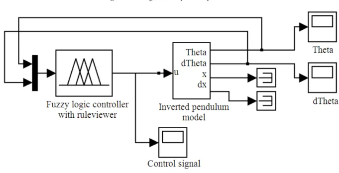
4. FUZZY LOGIC CONTROLLER

The Mamdani inference system was used as its graphical user-friendliness makes it easier to understand the controller’s logic. The previous knowledge that is required to control the system is formed by the following rules (Williams and Matsuoka, 1991):

• When the pendulum is falling away from the vertical and the angular speed is changing in the direction opposite to the fall, the pendulum will be forced to move in the same direction suggested by the angular speed

• When the car is moving at a certain distance from the center of the tracks and the pendulum is vertically oriented, the pendulum will tend to fall towards the center of the tracks

For simplicity, it will be considered here the stabilization of the pendulum, regardless of the position of the car. There were defined the following membership functions:

It were also determined seven rules as follows (Omatu and Ide, 1994):

• Rule 1: If θ = PM and θ = ZO, then u = PM • Rule 2: If θ = PS and θ = PS, then u = PS • Rule 3: If θ = PS and θ = NS, then u = ZO • Rule 4: If θ = NM and θ = ZO, then u = NM • Rule 5: If θ = NS and θ = NS, then u = NS • Rule 6: If θ = NS and θ = PS, then u = ZO • Rule 7: If θ_{= ZO and} θ_{= ZO, then u = ZO}

These rules can be summarized in the following table, called the fuzzy association matrix or knowledge matrix. The mambership functions are shown in Fig. 10.

The Fuzzy Inference System (FIS) was created as shown in Fig. 11.

The fuzzy control surface, presented in Fig. 12, was determined as follows:

To make use of the fuzzy controller, the block diagram in Fig. 13 was constructed with initial contions of 0.1 rad and 0.1 rad/s. The response is shown in Fig. 14.

It was obtained a good response as the pendulum is well-stabilized, slowly but without overshoot. Thus it is proved that the fuzzy controller has a correct behavior.

5. NEURAL NETWORK AS SYSTEM

IDENTIFIER

To show one of the applications of Neural Networks (NN) in the inverted pendulum problem. Now it was applied to the system under consideration. In first place, one must make some experiments and acquire representative points from the system. To obtain data from the stabilization area (vertical position), the robust open-loop controller described in the previous section. The system was excited in the desired region using perturbations to extend the data range, as shown in the block diagram in Fig. 15.

The training data consist of the state variables and the control signal, as shown in Fig. 16.

(8)

Fig. 8. Block diagram of the robust control with LQR

(9)

Fig. 10. Membership functions of the fuzzy controller

(10)

Fig. 12. Surface generated by the fuzzy controller

(11)

Fig. 14. Response of the fuzzy controller

(12)

Fig. 16. Training data

(13)

Fig. 18. Neural-network learning

(14)

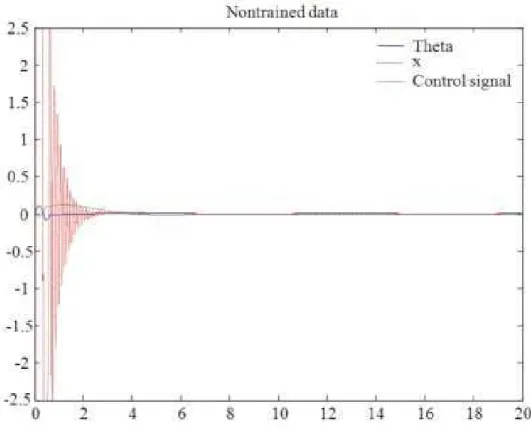
Fig. 20. Untrained data Thus it was chosen to use a Multilayer Perceptron (MLP)

with 20 hidden nodes with hyperbolic tangent functions and two linear nodes as output (Fig. 17).

Our MLP will estimate the following angle and position from the previous state and the control signal according to the function (Ravn and Poulsen, 2001) Equation 9:

y (t 1) g[y(t), y(t 1), y (t 2), u(t),..., u(t 1)]

+ = −

− − (9)

Where:

( )

(t) y t x(t) θ   =   

Levenberg-Marquardt training quickly (Hagan and Menhaj, 1994) reaches the error goal of 10-8, as shown in Fig. 18. Training data are well estimated (Fig. 19).

Neural networks are good learners of the training data, sometimes even too good as they only learn those data. To be certain that the NN really understood the system and not just the training data, additional data (called validation data) were generated as shown in Fig.

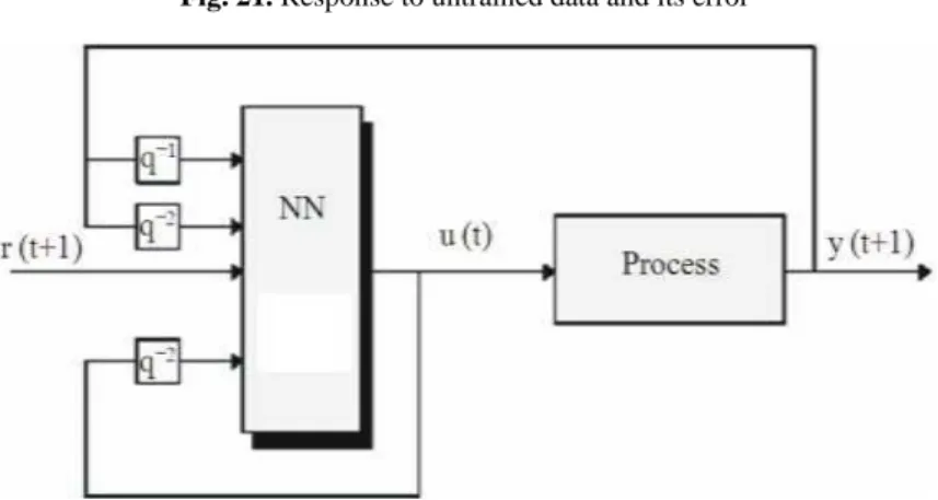
20 and the NN estimation achieved an error of less than 10-4, as shown in Fig. 21.

This is an excellent estimation, showing that neural networks are very good plant identifiers. Figure 22 shows a schematics of the Neural Network controller.

6. ANFIS CONTROLLER

(15)

Fig. 21. Response to untrained data and its error

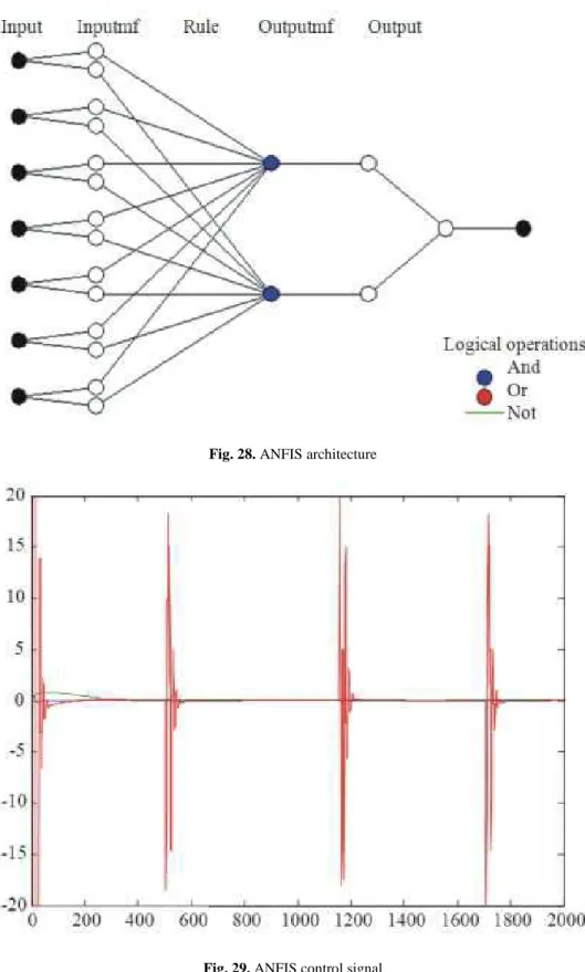
Fig. 22. Schematics of the controller with neural net-work The organization used is described as follows:

• Control with angle and position training in a time sequence with 8 inputs

The controller learns and operates in response to the previous system outputs and the previous signal from the controller itself. In this case, it will have seven inputs encompassing angles, positions and earlier control signals. The signal r(t+1) will consist exclusively of zeros, as the system’s reference signal.

Three different cases were considered: Random training, sub-clustering and grid partition. Each of them will now be described:

6.1. Random Training

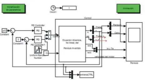
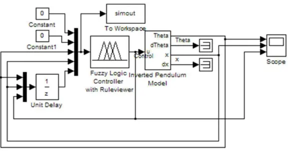
Training data were created by exciting the inverted pendulum system with random values, with no tuning of PID controllers, with the only purpose of finding the system response for different input types. A Simulink inverted-pendulum model with graphical interface presented by (Olguín, 2003) and represented in Fig. 23.

The Editor for the anfis system is presented in Fig. 24 which shows the training process when a cluster partition is used.

(16)

• C = length(entrenaCTRL)

• entrenaU = [entrenaCTRL(3:C,1:2),

entrenaCTRL(2:(C-1),1:2), entrenaCTRL(1:(C-2),1:3), entrenaCTRL(2:(C-1),3)]

• TrainU = [entrenaU(2:(C-2)/2,:)] • TestU = [entrenaU((C-2)/2:3*(C-2)/4,:)] • CheckU = [entrenaU(3*(C-2)/4:(C-2),:)] • anfisedit

• plot(entrenaU)

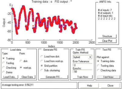
A grid-partition ANFIS controller was trained with 2 Gaussian-type membership functions per input, with a total of 7 inputs, a constant output and 50 training operations.

The error obtained, 0.56205, is acceptable because the control signal reaches ±200, an error of about 0.28%. Such error is compared with the reference value as shown in Fig. 25.

Fig. 23. Simulator of the inverted pendulum to obtain random data

(17)

Fig. 25. ANFIS editor showing trained data

Fig. 26. Block diagram of the ANFIS-controlled simu-lator There are gaps in the training data, so it does not

cover all possible values. Nevertheless, the network learns reasonably well from the system. To simulate the ANFIS controller, a block diagram was designed to feed the time-sequenced signals Fig. 26.

Results were rather unsatisfactory. Figure 27 shows that the system keeps within the desired zone for tenths of second, but remains unstable.

The topology of the ANFIS system is presented in Fig. 28-33 shows the control signal. One can infer that the ANFIS controller is capable of controlling the system, but more training in the stabilization zone is required. As the random signals do not cover specifically well this area, a controller that keeps them in the desired zone is required.

6.2. Sub-Clustering

This approach to creating a fuzzy network consists of dividing training data among different zones and creates membership rules between them. With the standard parameters:

• Influence range: 0.5 • Compression factor: 1.5 • Acceptance rate: 0.5 • Rejection rate: 1.5

(18)

for angle and position, respectively. In addition, impulse perturbations were introduced that provide the change of reference for the car’s position. The control signal was saturated at ±20 and the following result was obtained:

The signal was prepared using the EntrenaU program, using the following expresión Equation 11:

1 y(t 1), y(t),..., y

ˆu(t) g

(t n 1), u(t 1),..., u(t m)

−  + 

=  _{− +} ₋ ₋ 

  (11)

And the following code:

• entrenaCTRL = Ucontrollim • C = length(entrenaCTRL)

• entrenaU = [entrenaCTRL(3:C,1:2),

entrenaCTRL(2:(C-1),1:2), entrenaCTRL(1:(C-2),1:3), entrenaCTRL(2:(C-1),3)]

• TrainU = [entrenaU(2:(C-2)/2,:)] • TestU = [entrenaU((C-2)/2:3*(C-2)/4,:)] • CheckU = [entrenaU(3*(C-2)/4:(C-2),:)]

Training was made with half of the available data, with testing and cheking made with the remaining half. Sub-clustering training was made with the ANFISEDIT routine using the following parameters:

A 7-input network was generated with two membership functions per input and a linear output of the form:

Training was performed in 50 iterations with a hybrid optimization approach.

Once the ANFIS was trained, it was simulated with the following block diagram:

The system was capable of controlling initial conditions of 0.1 rad and 0.1 m, even for initial conditions of 0.3 rad and 0.1 m. However, it never reaches total stabilization as it oscillates, although it manages to keep the pendulum in the desired, vertical region. It was also tested changing the output condition to constant, but that means only two rules and becomes nonfunctional.

6.3. Grid Partition

Training data were determined by the robust controller previously obtained. Care was taken to ensure that the control would not only find the stabilization data, but also that it would become momentarily unstable to

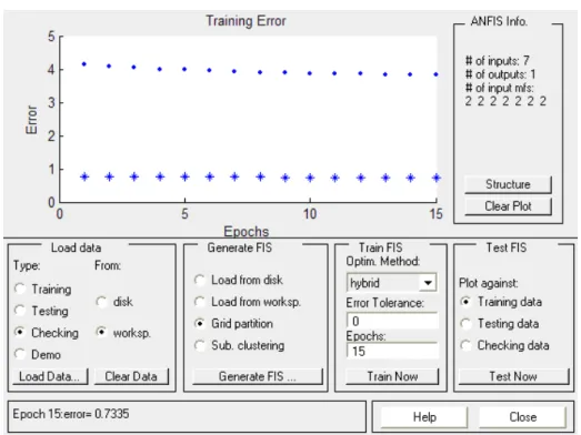
determine a larger response range. Then a system with two Gaussian-type membership functions was created for the 7 inputs and a constant output. The network creates many rules by itself, as shown in Fig. 34.

It was trained with an error of 0.7335, as shown in Fig. 35. Nevertheless, the simulation response is unstable, as shown in Fig. 36. The output is made of 128 parameters (128 constant-type rules).

Trying to improve this type of controllers, a new test was performed for a more complex system. The same parameters of the previous case were used with a linear output. The resulting training had an error of 0.59917, but the result is still unsatisfactory, as shown in Fig. 37 and the control topology is presented in Fig. 38.

6.4. Control with 8-Input Time-Sequence State

Training

This control is trained with the desired signal and the previous system output; the desired signal when using the controller is the zero matrix. Learning is simplified but there are fewer conditions showing the state of the system. The training data were obtained with the same robust controller. These data were reordered in such a way that the current (theta, dtheta, x, dx) and future states were considered in the training of the controller. The following code was used:

• %8 ENTRADAS, ESTADO +1 (THETA,

DTHETA, X, DX) Y ESTADO ACTUAL • entrenaXref = UcontrollimX

• D = length(entrenaXref)

• entrenaUXref =

[entrenaX(3:D,1),entrenaX(3:D,2),entrenaX(3:D,3),

entrenaX(3:D,4),entrenaX(2:(D- 1),1),entrenaX(2:(D-1),2),entrenaX(2:(D-1),3),entrenaX(1:(D-2),4),entrenaX(2:(D-1),5)] • TrainUXref = [entrenaUXref(2:(D-2)/2,:)] • TestUXref = [entrenaUXref((D-2)/2:3*(D-2)/4,:)] • CheckUXref = [entrenaUXref(3*(D-2)/4:(D-2),:)]

Training data are shown in Fig. 39. A grid-partition ANFIS was also built of the form shown in Fig. 40.

(19)

other examples Fig 42-44. As expected, it did not work (but it was worthwhile to try it!).

6.4. Control with 4-Input State Training

This control is the simplest of its type. It is trained and executed with only the state of the system. It can be used because the reference does not change in time. It is the simplest method, so its implementation may help in the next stage using genetic algorithms.

Table 2. Represents the fuzzy association matrix in which the negative values of the consequences are concentrated in the upper zone of the table (NS and

NM), positive values are in the lower zone of the table (PS and PM) and Zero in the diagonal line (ZO). Those consequences are the representative values for the inputs signals (Θ and ∆Θ).

Table 2. Fuzzy association matrix of the fuzzy controller

θ\ θ NS ZO PS

NM NM

NS NS ZO

ZO ZO

PS ZO PS

PM PM

(20)

Fig. 28. ANFIS architecture

(21)

Fig. 30. ANFIS network architecture

(22)

Fig. 32. Block diagram of the system with ANFIS controller with time-dependent state

(23)

Fig. 34. ANFIS architecture with grid partition

(24)

Fig. 36. ANFIS results for grid partition

(25)

Fig. 37. Grid-partition ANFIS simulation results

(26)

Fig. 29. Training data for the controller

(27)

Fig. 41. Grid-partition ANFIS editor

(28)

Fig. 43. Schematics of the ANFIS controller

(29)

Fig. 46. Sub-clustering ANFIS editor

(30)

Three different forms were implemented: Differential control as a function of k, continuous control with a small number of training data and continuous control with a larger number of training data. Only the best example of each form will be analyzed here.

Differential control as a function of k Given that this control works with the state data in time K, the discretization of the training data was considered in such a way that the derivative would be the diference between k and k+1. This was done with the following code:

• entrenaX = Ucontrollim • D = length(entrenaX)

• entrenaUX = [entrenaX(2:(D-1),1),-entrenaX(2:(D- 1),1)+entrenaX(1:(D-2),1),entrenaX(2:(D-1),2),-

entrenaX(2:(D-1),2)+entrenaX(1:(D-2),2),entrenaX(2:(D-1),3)]

• TrainUX = [entrenaUX(2:(D-2)/2,:)] • TestUX = [entrenaUX((D-2)/2:3*(D-2)/4,:)] • CheckUX = [entrenaUX(3*(D-2)/4:(D-2),:)]

The training data were generated. Training was performed in several forms and was simulated with the block diagram shown in Fig. 45, with is simplified as the

derivative must be equal to the change between the previous and current states and the current value is the desired (zero) value. Thus, the derivative is simply the negative value of the previous output.

Now it will be analyzed several tests from the configuration and training of the ANFIS.

6.5. Sub-Clustering

The following parameters were used:

Training error has the value 2.0805. The result becomes unstable after a few seconds.

The training of the ANFIS was done by sub-clustering , the editor is presented in Fig. 46 and the results of the ANFIS controller’s simulation are shown in Fig. 47.

6.6. Continuous With Few Training Data

(31)

state. Once again, the robust controller data were obtained and are shown in Fig. 48.

The training data were generated according to:

• % 4 ENTRADAS, ESTADO THETA, DTHETA, X,

DX

• entrenaX = UcontrollimX • D = length(entrenaX)

• entrenaUX = [entrenaX(2:(D-1),1),entrenaX(2:(D-

1),2),entrenaX(2:(D-1),3),entrenaX(1:(D-2),4),entrenaX(2:(D-1),5)]

• TrainUX = [entrenaUX(2:(D-2)/2,:)] • TestUX = [entrenaUX((D-2)/2:3*(D-2)/4,:)] • CheckUX = [entrenaUX(3*(D-2)/4:(D-2),:)]

The ANFIS controller with grid partition was trained with 2 membership functions for each of the four inputs, with 1 linear output. Fig. 49. Presets the ANFIS editor for grid partition

The rules are shown as follows (Fig. 50):

Direct simulation was performed, with the current state provided as feedback. Notice that the controller does not depend on the system error, but on its current conditions and from that information it chooses the new signal to stabilize the plant; Fig. 51. shows the ANFIS simulator’s block diagram. Fig. 52 exemplifies the ANFIS simulation results in which smooth merging responses are reached.

A test was made for 0.1 rad and 0.1 m initial conditions. The result is shown as follows. It totally stabilizes in 6 sec.

On the other hand, with different initial conditions, like 0.3 rad and 0.1 m, the system becomes unstable, as shown in Fig. 53.

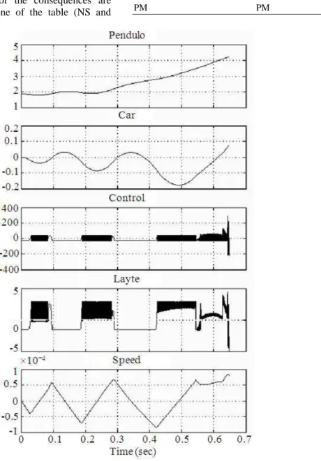
The Fig 53 and 54 gives the results when the initial conditions are postive and negative and how those conditions affects the whole system Fig. 55-72.

Finally, direct state feedback of the system was again tested, but now with more training data. The same data of the robust controller were used, divided in two groups. The first half was used for training and the second half was further divided in two, with one quarter of the total data to test and the last quarter to check. The same logic was used as with the earlier controllers, but now data were created for both initial and positive initial conditions. Training was performed first with the response to positive initial conditions and then to negative initial conditions. The same was done for the test and evaluation of the controller.

The data provided are:

With sub-clustering, 30 iterations and the following parameters:

• Influence range: 0.2 • Acceptance rate: 0.2 • Rejection rate: 0.1

• A network with the following structure was obtained It was simulated for initial conditions of 0.3 rad and 0.3 m, obtaining the following result.

6.7. Then, with -0.3 rad and -0.3 m

Upon detailed analysis, the stable-state error for theta is 0 and for x is 5e-3.

This last controller is the one which worked best in accordance to the established requirements and was prepared for optimization with genetic algorithms.

For each control type, different parameters were tested about the network build-up, with different training data. This means that the search for an efficient controller may be very complex, aside from the fact that no established story was made up except for the observation of the results while varying the results.

7. ANFIS CONTROLLER OPTIMIZED BY

GENETIC ALGORITHMS

Genetic algorithms are used to optimize a system without the use of derivatives, by a defined criterion, with parameters such as the mutation and crossing rate and choices such as the coding, selection and evaluation methods for each member of the population (Omatu et al., 1995). For a more detailed description of genetic algorithms, the reader is direct to (Hassanzadeh et al., 2008)

It with the ANFIS controller previously defined. Only the parameters of the two linear output functions (5 parameters for each output). The controller is described in the following block diagram.

The inverted pendulum model provides the initial conditions.

(32)

Fig. 49. ANFIS editor for grid partition

(33)

Fig. 51. ANFIS simulator’s block diagram

(34)

Fig. 53. Results of the ANFIS simulation with other inicial conditions

(a)

(b)

(35)

Fig. 55. ANFIS editor for sub-clustering

(36)

Fig. 57. Response of the system to positive initial con-ditions

(37)

Fig. 59. Block diagramo of the system optimized with a genetic algorithm

Fig. 60. Optimization with genetic algorithm in 100 iterations (Error vs generations)

(38)

Fig. 62. System response to positive initial conditions

(39)

Fig. 64. System response to negative initial conditions

(40)

(a)

(b)

Fig. 66. System response to two different initial conditions (a) After GA with positive initial conditions and (b) After GA with Negative initial conditions Time in [ms]

(41)

Fig. 68. System response to positive initial conditions

(42)

Fig. 70. System error from the new weighted quadratic criterion

(43)

(a)

(b)

Fig. 72. System response for two different initial conditions (a) positive and (b) negative The base code of the genetic algorithm used in this

paper is presented in (Storn and Price, 1997). The genetic algorithm was worked in all the simulations with the following parameters:

• VTR-Value To Reach, it is a condition for stopping which, in our case, the error criterion establishes to be of 1×10-3, under the assumption that such value would never be reached

• Maximum number of iterations-Number of generations, this was the main stopping condition of the algorithm

• D-Number of parameters to modify by the system; in our case there were 10 such parameters

• XVmin-Inferior-limit vector for the initial population; it was-10% the value of each output parameter for the initial ANFIS

• XVmax-Superior limit vector for the initial population; it was +10% the value of each output parameter for the initial ANFIS

• NP-Number of members of the population. There were used 15*D, i.e., 150 members for each population • F-Step value between iterations; a value between 0

and 2 is suggested-it was chosen 1

• CR-probability of crossing, should be between 0 and 1, for which it was chosen 0.4

Strategy-The algorithm allows one to choose among many strategies, but the one that served us best was an exponential (non-binary) value coding with a rand-to-best logic, which reinforces from the random values those that gave a better response.

Refresh-It measures the number of generations that are counted before presenting results. This was an unimportant parameter from the optimization point of view, but it helped us to observe the process. It was used it to generate optimization graphs.

Several genetic-algorithm programs were created with different systems and different iteration numbers, namely:

• System with initial conditions -0.3 rad and -0.3 m, up to 100 iterations

• System with initial conditions 0.3 rad and 0.3 m, up to 2000 iterations

• System with initial conditions both positive and negative (±0.3 rad and ±0.3 m), up to 200 iterations • System with initial conditions both positive and

(44)

• System with initial conditions both positive and negative (±0.5 rad and ±0.5 m), up to 1000 iterations with a weighted stopping criterion

6.8. Now, it will be Analyzed

System with initial conditions -0.3 rad and -0.3 m, up to 100 iterations.

With the system having initial conditions of -0.3 rad and -0.3 m, the following function is to be optimized Equation 12:

2 2

error=20 *

∑

theta +10 *

∑

x (12)

where, theta and x are the output values in each simulation time. A weight of twice the error is given for the angle considered with respect to position to enhance the controller’s operation over this variable. The simulation was executed with Simulink and the values of theta and x were exported in matrix form. The optimization was made for 100 iterations:

The optimized parameters, which are the constants in the linear output equations of the Sugeno controller, are given by:

• best(1) = 34.995418 • best(2) = 3.882741 • best(3) = 3.441896 • best(4) = 4.816650 • best(5) = 0.074609 • best(6) = 18.771968 • best(7) = 5.367916 • best(8) = 21.764996 • best(9) = 10.569450 • best(10) = -0.256071

After running the simulation with initial conditions of -0.3 rad and -0.3 m, it was obtained:

With positive initial conditions of 0.3 rad and 0.3 m, we obtained:

System with initial conditions 0.3 rad and 0.3 m, up to 2000 iterations

It is handled in the same way as the previous iteration, but now with positive initial conditions (0.3 rad and 0.3 m), up to 2000 iterations (generations), as follows:

It took the algorithm 19 h to finish, executing some 300,000 evaluations in the simulator (block diagram). The parameters thus obtained were:

• best(1) = 46.415248 • best(2) = 0.443056

• best(3) = 24.635170 • best(4) = -1.163018 • best(5) = -7.951112 • best(6) = 7975.784165 • best(7) = 297.404686 • best(8) = 3420.556959 • best(9) = 364.341177 • best(10) = -1.014442

6.9. It is Obtained

System with initial conditions both positive and negative (±0.3 rad and ±0.3 m), up to 200 iterations.

It was handled in a similar way as the previous one, but taking care that the optimization has at the same time an evaluation with positive and negative initial conditions. This was achieved by running two 5-sec simulations for positive and negative initial conditions. Both were executed every time that the optimization criterion was evaluated and both arrays were exported to satisfy the criterion Equation 13:

2 pos neg 2

pos neg

error 20 * (theta theta )

10 * (x x )

= + +

+

∑

(13)

This case was executed with 200 iterations (generations).

The optimized parameters are:

• best(1) = 38.348628 • best(2) = 4.352005 • best(3) = 6.595191 • best(4) = 6.084092 • best(5) = 0.315752 • best(6) = 21.473104 • best(7) = 6.225609 • best(8) = 20.732177 • best(9) = 10.852273 • best(10) = -0.450915

6.10. It is Obtained

System with initial conditions both positive and negative (±0.5 rad and ±0.5 m), up to 2000 iterations.

With more critical positive and negative initial conditions (±0.5 rad and ±0.5 m), it was trained for 2000 iterations.

The system was evaluated 600,000 times; the following values were obtained:

(45)

• best(3) = 31.878815 • best(4) = 69.917063 • best(5) = 0.114835 • best(6) = 402.254374 • best(7) = 5.614562 • best(8) = 190.474634 • best(9) = 33.375531 • best(10) = 30.360559

6.11. Upon Execution, it Turns out to be

Unsatisfactory

System with initial conditions both positive and negative (±0.5 rad and ±0.5 m), up to 1000 iterations with a weighted stopping criterion.

The optimization technique that worked best was the fifth one, which was optimized with both positive and negative initial conditions (±0.5 rad and ±0.5 m), with 1000 iterations. A weighted stopping criterion was especially used.

Trying to get out from the transient as soon as possible and eliminate any steady-state error, the evaluation criterion was changed for another that weighted error with respect to time, that is, weighting incremented linearly with time at a rate of 0.1 per millisecond, beginning with a y-intercept of 1 so as not to neglect initial conditions:

This is achieved with the command:

• ponderacion=1:.1:length(simout)/10

• where simout are the output values of the simulation For example, for the ANFIS controller without optimization with GA’s, the error in theta will be:

• errorcuadradoponderado=power(simout(:,1).*ponder ac’,2)

• plot(ponderac,errorcuadradoponderado)

Summarizing, the minimization criterion that is satisfied is Equation 14:

2 pos neg

error 20 * pond * ( ) 10 * pond * (x x )

= θ + θ

+ +

∑

(14)

With the given initial conditions (±0.5 rad and ±0.5 m) and 1000 iterations (generations), one gets:

This optimization results gave:

• best(1) = 41.116217 • best(2) = 6.484782 • best(3) = 11.042188

• best(4) = 8.654519 • best(5) = -0.795826 • best(6) = 340.727888 • best(7) = 79.851994 • best(8) = 53.532277 • best(9) = 31.549543 • best(10) = 1.838144

This is an excellent optimization of critical initial conditions.

7. CONTRIBUTIONS TO THE STATE OF

THE ART

An adequate integration of the intelligent control methods allows to design simpler and optimal control for complex systems. A correct integration of the ANFIS method with genetic algorithms is presented.

This study proposes the application to the inverted-pendulum problem of an existing control method (called the “genetic-ANFIS controller” or “neural-fuzzy-with-genetic-algorithms controller), which relies in some of the latest advances of intelligent control. Also this study shows the complete methodology for finding the correct design of the controller.

8. CONCLUSION

Intelligent control provides a new area for solving control problems. Its advantages are due to the integration of computers to generate intelligent and adaptive algorithms, or by a more human-like logic than that attained with traditional control. Its efficacy has been proved by simulation, implementing in an inverted pendulum its main components, such as fuzzy controllers, neural networks and genetic algorithms, as well as the interaction between all of them with the genetic-ANFIS controller.

This study reached many of its objectives, providing a good training ground for intelligent control, but it also presented a remarkable challenge given the evolution of tools and methodologies.

(46)

methodology will be found that may be used in any plant regardless of its characteristics. It will be possible to learn from the plant as time goes on, eliminating the need for mathematical models.

9. REFERENCES

Chen, S.C. and W.L. Chen, 2003. Output regulation of nonlinear uncertain system with nonminimum phase via enhanced RBFN controller. IEEE Trans. Syst.

Man Cybernet., 33: 265-270. DOI:

10.1109/TSMCA.2003.810907

Cho, H.T. and S. Jung, 2003. Balancing and position tracking control of an inverted pendulum on a x-y plane using decentralized neural networks. Proceedings of the IEEE/ASME International Conference on Advanced Intelligent Mechatronics, Jul. 20-24, IEEE Xplore Press, pp: 181-186. DOI: 10.1109/AIM.2003.1225092

DECE, 2003. Control Tutorials for MATLAB and Simulink. Department of Electrical and Computer Engineering, Utah State University.

Bishop, R.H.C. and R.C. Dorf, 1999. Teaching modern control system design. Proceedings of the 38th IEEE Conference on Decision and Control, Dec. 7-10, IEEE Xplore Press, Phoenix, AZ., pp: 364-369. DOI: 10.1109/CDC.1999.832803

Gao, Y. and M.J. Er, 2003. Online adaptive fuzzy neural identification and control of a class of MIMO nonlinear systems. Fuzzy Syst. IEEE Trans., 11: 462-477. DOI: 10.1109/TFUZZ.2003.814830033 Hassanzadeh, I., S. Mobayen and A. Harifi, 2008.

Input-Output Feedback Linearization Cascade Controller Using Genetic Algorithm for Rotary Inverted Pendulum System. Am. J. Applied Sci., 5: 1322-1328. DOI: 10.3844/ajassp.2008.1322.1328

Hagan, M.T. and M.B. Menhaj, 1994. Training feedforward networks with the marquardt algorithm. IEEE Trans. Neural Netw., 5: 989-993. DOI: 10.1109/72.329697

Harrison, R.F., 2003. Asymptotically optimal stabilising quadratic control of an inverted pendulum. IEE Proc. Control Theory Applic., 150: 7-16. DOI: 10.1049/ip-cta:20030014

Inoue, H., K. Matsuo, K. Hatase, K. Kamei and M. Tsukamoto et al., 2002. A fuzzy classifier system using hyper-cone membership functions and its application to inverted pendulum control. Proceedings of the IEEE International Conference on Systems, Man and Cybernetics, Oct. 6-9, IEEE Xplore Press. DOI: 10.1109/ICSMC.2002.1175598

Jang, J.S.R., 1992. Self-learning fuzzy controllers based on temporal backpropagation. IEEE Trans.

Neural Netw., 3: 714-723. DOI:

10.1109/72.159060

Jang, J., 1993. ANFIS: Adaptive-network-based fuzzy inference system. IEEE Trans. Man Cybernet. Syst., 23: 665-685. DOI: 10.1109/21.256541 Jang-Sun-Mizutani, 1997. Neuro-Fuzzy and Soft

Computing. 1st Edn., Prentice-Hall, Upper Saddle River, ISBN-10: 0132610663, pp: 614.

Ji, C.W., F. Lei and L.K. Kin, 1997. Fuzzy logic controller for an inverted pendulum system. IEEE proceedings of the International Conference on Intelligent Processing Systems, Oct. 28-31, IEEE Xplore Press, Beijing, pp: 28-31. DOI: 10.1109/ICIPS.1997.672762

Jacobs, R.A. and M.I. Jordan, 1993. Learning piecewise control strategies in a modular neural network architecture. IEEE Trans. Syst. Man Cybernet., 23: 337-345. DOI: 10.1109/21.229447 Jung, S. and S.B. Yim, 2000. Reference compensation

technique using neural network for controlling large x-y table robot. Proceedings of the International Symposium Robotics and Automation., (SRA’ 00), pp: 461-466.

Kitamulra, S. and M. Saitoh, 1990. Stability of inverted pendulum by neuro-PID control with genetic algorithm. Proceedings of the IEEE International Joint Conference on Neural Networks, May 4-9, IEEE Xplore Press,

Anchorage, AK., pp: 61-61. DOI:

10.1109/IJCNN.1998.687191

Kouda, N., N. Matsui and H. Nishimura, 2002. Control for swing-up of an inverted pendulum using qubit neural network. Proceedings of the 41th SICE Annual Conference, Aug. 5-7, IEEE

Xplore Press, pp: 765-770. DOI:

10.1109/SICE.2002.1195253

Lam, H.K., F.H. Leung and P.K.S. Tam, 2003. Design and stability analysis of fuzzy model-based nonlinear controller for nonlinear systems using genetic algorithm. IEEE Trans. Syst. Man

Cybernet., 33: 250-257. DOI:

10.1109/TSMCB.2003.810440

Lundeberg, K., 1994. The inverted pendulum system. 1994-2002.

Messner, B. and D. Tilbury, 1999. Control Tutorials for Matlab and Simulink. 1st Edn., Addison-Wesley, ISBN-10: 0201477009, pp: 32.

(47)

Mohanlal, P.P. and M.R. Kaimal, 2002. Exact fuzzy modeling and optimal control of the inverted pendulum on cart. Proceedings of the 41th IEEE Conference on Decision and Control, Dec. 10-13, IEEE Xplore Press, pp: 3255-3260. DOI: 10.1109/CDC.2002.1184373

Nørgaard, M., 2000a. Neural network based control system design toolkit. ver. 2” Tech. Report. 00-E-892, Department of Automation, Technical University of Denmark.

Nørgaard, M., 2000b. Neural network based system identification toolbox. Tech. Report. 00-E-891, Department of Automation, Technical University of Denmark.

Olguín, E., 2003. Simulación en MATLAB de péndulo invertido, con etapa gráfica. Abril.

Olguín, E., 2000. Modelado matemático del péndulo invertido.

Omatu, S. and T. Ide, 1994. Stabilization of inverted pendulum by neuro-control. Proceedings of the IEEE International Conference on Neural Networks, IEEE World Congress on Computational Intelligence, Jun. 27- Jul. 2, IEEE Xpore Press,

Orlando, FL., pp: 2367-3272. DOI:

10.1109/ICNN.1994.374589

Omatu, S., S. Deris and K. Kitagawa,1995. Stabilization of inverted pendulum by the genetic algorithm. Proceedings of the IEEE International Conference on Intelligent Systems for the 21st Century Systems, Man and Cybernetics, Oct. 22-25, IEEE Xplore Press, Vancouver, BC., pp: 4372-4377. DOI: 10.1109/ICSMC.1995.538481 Omatu, S., T. Fujinaka and M. Yoshioka, 2000.

Neuro-PID control for inverted single and double pendulums. Proceedings of the IEEE International Conference on Systems, Man and Cybernetics, Oct. 8-11, IEEE Xplore Press, Nashville, TN., pp: 3685-2690. DOI: 10.1109/ICSMC.2000.884401

Pal, T. and N.R. Pal, 2003. SOGARG: A self-organized genetic algorithm-based rule generation scheme for fuzzy controllers. IEEE Trans. Evolut. Comput., 7: 397-415. DOI: 10.1109/TEVC.2003.815377

Storn, R. and K. Price, 1997. Differential evolution-a simple and efficient heuristic for global optimization over continuous spaces. J. Global Optimiz., 11: 341-359. 10.1023/A:1008202821328

Ravn, N. and H. Poulsen, 2001. Neural Networks for Modelling and Control of Dynamic Systems. 1st Edn., Springer.

Riedmiller, M., 1993. Controlling an inverted pendulum by neural plant identification. Proceeding of the International Conference on Systems, Man and Cybernetics, Systems Engineering in the Service of Humans, Conference, Oct. 17-20, IEEE Xplore Press, Le Touquet, pp: 473-478. DOI: 10.1109/ICSMC.1993.390758

Saifizul, A.A., Z. Zainon, N.A.A. Osman, C.A. Azlan and U.F.S.U. Ibrahim, 2006. Intelligent Control for Self-erecting Inverted Pendulum Via Adaptive Neuro-fuzzy Inference System. Am. J. Applied Sci., 3:1795-1802. DOI: 10.3844/ajassp.2006.1795.1802 Sazonov, E.S., P. Klinkhachorn and R.L. Klein, 2003.

Hybrid LQG-neural controller for inverted pendulum system. Proceedings of the 35th Southeastern Symposium on, Mar. 16-18, IEEE Xplore Press, pp: 206-210. DOI: 10.1109/SSST.2003.1194559

Takagi, T. and M. Sugeno, 1985. Fuzzy identification of systems and its applications to modeling and control. IEEE Trans. Syst. Man Cybernet., 15: 116-132. DOI: 10.1109/TSMC.1985.6313399

Williams, V. and K. Matsuoka, 1991a. Learning to balance the inverted pendulum using neural networks. IEEE Int. Joint Conf., 1: 214 -219. Yang, R., Y.Y. Kuen and Z. Li, 2000. Stabilization of a