Neural feedback linearization adaptive control for affine nonlinear systems based on neural network estimator

Vol. 8, No. 3, November 2011, 307-323

Neural Feedback Linearization Adaptive

Control for Affine Nonlinear Systems

Based on Neural Network Estimator

Mohamed Bahita

, Khaled Belarbi

Abstract: In this work, we introduce an adaptive neural network controller for a class of nonlinear systems. The approach uses two Radial Basis Functions, RBF networks. The first RBF network is used to approximate the ideal control law which cannot be implemented since the dynamics of the system are unknown. The second RBF network is used for on-line estimating the control gain which is a nonlinear and unknown function of the states. The updating laws for the combined estimator and controller are derived through Lyapunov analysis. Asymptotic stability is established with the tracking errors converging to a neighborhood of the origin. Finally, the proposed method is applied to control and stabilize the inverted pendulum system.

Keywords: Adaptive control, Control gain estimation, Feedback linearization, Radial basis function network.

1 Introduction

Adaptive control seems today a natural strategy to tackle the stabilization and tracking of highly uncertain nonlinear dynamical systems. Although linear systems are very well understood and controlled, linear control is not enough to guarantee stability and performance of nonlinear systems.

A milestone in the extension of linear control techniques to nonlinear systems has been the development of nonlinear geometric control. Recent research involving differential geometric methods [12, 13, 17] has rendered the design of controllers for a class of nonlinear systems somewhat systematic. This nonlinear control theory, called feedback linearization, is based on coordinate transformations by which a class of nonlinear systems can be transformed into linear systems through feedback. With the advent of feedback linearization, adaptive control found its way into nonlinear control. The combination of adaptive control and feedback linearization applied to flight control can be found in [16]. In most of the classical adaptive control literature it is common to

1_{Faculty of Hydrocarbons and Chemistry (FHC), University of Boumerdes, Boumerdes 35000, Algeria;}

E-mail mbahita@yahoo.fr 2

assume the unknown dynamics to have a known structure with unknown parameters entering linearly in the dynamics. The linear parameterization of unknown dynamics poses serious obstacles in adopting adaptive control algorithms in practical applications, because it is difficult to fix the structure of the unknown nonlinearities. This fact has been the motivating factor behind the interest in on-line function approximators to estimate the unknown function. The most common function approximators used in adaptive control are artificial neural network and fuzzy logic systems.

The ability of neural networks to approximate uniformly continuous functions has been proven in several articles [6, 7, 10, 11]. Neural networks (NNs) for identification and control were first proposed by Narendra and Parthasarathy [14]. Results in this initial research were limited to simulation and no proofs of stability in the closed loop were provided. Tzirkel and Fallside proposed the use of neural network control providing proof of stability [19].

In the majority of proposed adaptive controller a complementary term, called supervisory term, is added to the output of the fuzzy inference system or of the neural network system controller in order to guarantee global stability using Lyapunov theory [20]. When the system is operating within a prescribed range, the supervisory controller is turned off. The difference between the various methods lies in the structure of the model and in the form of the supervisory term, the approximated control law is based on the certainty equivalence approach while the supervisory term can take different forms, but most often, it is based on the sliding mode technique. Sanner and Slotine first proposed Radial Basis Function (RBF) NNs for control of affine systems and provided rigorous analysis of stability. They introduced a sliding mode component in the control law for keeping the evolving dynamics within the predetermined compact set of interest [15].

In this work, we introduce an alternative adaptive controller for affine nonlinear systems without the use of the supervisory control term. The architecture employs two RBF networks: the first RBF network is used to approximate the ideal control law which cannot be computed, because the system dynamics are unknown, and the second network is used to estimate the virtual control gain which is an unknown nonlinear function of the states.

concerned only with the connections weights and the centres of the basis functions are fixed offline. In this work, we propose to online adjust both the centres of the basis functions and the connections weights.

The centres of the RBF networks are adapted on line using the k-means algorithm [5, 21]. The global stability of the resulting closed loop system is established and the updating laws for the parameters are derived using Lyapunov stability theory.

This paper is organised as follows: in Section 2, the problem formulation is introduced, in Section 3, the stability analysis is developed and the adaptive laws are derived, in Section 4, the indirect adaptive RBF-RBF controller is used in simulation for controlling the inverted pendulum system. Section 5 concludes the paper.

2 Problem

Formulation

Consider the following nonlinear system

( )n _{( , ,...,} (n 1)_{) ( ) ,}

x = f x x x − +b x u y=x, (1)

where u ∈R and y∈R are the input and output of the system respectively, ( )

f x and b x( ) are unknown nonlinear functions. We assume that the state

vector ( 1)

1 2

( , ,..., )T ( , ,... n )T n n

x= x x x = x x x − ∈R is available for measurement. The control objective is to force ( )y t to follow a given bounded reference signaly t_m( ), under the constraints that all involved signals must be bounded. Define the error vector as

( 1)

( , ,..., n )T n

e= e e e − ∈R . (2)

In order to design the controller we consider the following two steps: Step 1: We choose u to cancel the nonlinearities in the nonlinear system so that the closed-loop dynamics is in a linear form, and guarantees tracking convergence, as we have mentioned previously, this is called feedback linearization [12, 13, 17]. If the functions f x( ) and b x( ) are known and assuming ( )b x to be non zero (this is an usual assumption) then from (1), the optimal control law is:

1

( ( ))

( )

u v f x

b x

•_{= −}

. (3)

Substituting (3) into (1), we can cancel the nonlinearities and obtain the simple input-state relation:

( )n

Step 2: We choose the artificial input v (an equivalent input) as a simple linear pole-placement controller = ( )n − T

m

v y K e that guarantees the stability of the overall system, with

0 1 1

( , ,..., )T n n

K= k k k ₋ ∈R (5)

chosen so that the polynomial:

1

1 0 0

n n

n

s +k ₋s − + +k = (6)

has all its roots strictly in the left-half complex plane. Then the control law is:

( )

1

( ( ))

( )

n T m

u y K e f x

b x

• _{= − − . (7)}

Since e= −y y_m, then:

( )n ( )n ( )n m

e =y −y . (8)

Substituting (7) into (1), using (8) we have:

( ) ( 1)

1 0 0

n n

n

e +k ₋e − + +k e= , (9)

which implies that lim ( )e t →0 as t→ ∞, i.e., exponentially stable dynamics [18], which is the main objective of control. However, since f x( ) and b x( ) are

unknown, the ideal control u• of (7) cannot be implemented. Our purpose is to design an RBF network u x( , )θ to approximate this ideal control law u• and based on this approximation we design a second RBF network to approximate the unknown function b x( ) (the virtual control gain). The following sections describe and analyze the proposed controller.

3

The Neural Adaptive Controller

As mentioned above, the proposed adaptive controller is composed of two RBF networks. The RBF network can be considered as a two-layer network with one hidden layer. The output depends linearly on the weights, the training is thus a linear optimization problem [8]. More explicitly, the RBF network performs the transformation:

: n

r

f R →R,

with:

(

)

2 2

1

( , ) ( ),

nr

T

b i bi b i i

i

b x x x c

=

θ =

∑

layer, c_i are centres of the basis functions, nris the number of basis functions. The most common basis function is the Gaussian function:

2 2

( ) exp 2

r

r ⎛− ⎞

ψ = _{⎜ ⎟}

σ

⎝ ⎠, (11)

with r= −x c_{i 2}, σ is an associated constant to the function ψ( )r and represents the width of the Gaussian function. Although the RBF network is usually considered linear parameterized, by adjusting the centres and the widths this type of neural network structure becomes nonlinearly parameterized. In this work, we propose to online adjust both the centres of the basis functions and the connection weights. The connection weights of the two RBF networks: the controller and the estimator are to be adapted and will be represented respectively by the vectors θ and θ_b. The k-means algorithm is used for the centres adjustment. The k-means algorithm [5, 21] is an unsupervised training method for data clustering. It consists in dividing the input space into nr classes as follows:

1. Choose a number of classes (n_r basis functions in our case). 2. Initialise the centres of the basis functions.

3. Compute the Euclidean distances between the centres of each basis function and the input vector x, i.e.

2

( )= − _i , =1, 2,…, _r

dist i x c i n , (12)

then adjust the vector of centres c_i which corresponds to the minimum distance

2

( ) min _i

dist j = x−c using the following adaptation law [5]:

(

)

( ) ( 1) ( ) ( ) ( 1)

j j j

c t =c t− + δ t x t −c t− (13)

where j is the index of the basis function which corresponds to the minimum Euclidean distance dist j( ) and ( )δt is a gain belonging to the interval [0 1], and which tends to zero as t→ ∞. One adaptation law for this parameter as given in [2] is the following:

( 1) ( )

1 int( )

δ −

δ =

+ _r

t k

t n , (14)

3. 1 The RBF adaptive controller

Now, supposing that the control u in (1) is the output of the first RBF controller ( , )u x θ , i.e., u=u x( , )θ , then (1) becomes:

( )n _{( ) ( ) ( , )}

x = f x +b x u xθ , (15)

now adding and subtracting _{b x u( )} * _{to (15) we will have:}

( )n _{( ) ( ) ( , ) ( ) ( )}

x = f x +b x u x θ +b x u•−b x u•. (16)

Substituting (7) into (16), we obtain:

( ) ( )

( ) ( ) ( , ) ( ) ( )

n n T

m

x = f x +b x u x θ −b x u•+y −K e− f x , (17)

thus:

( )n ( )n T _{( )( ( , ) )} m

x −y +K e=b x u x θ −u• . (18)

Based on y=x in (1), using (2) and (8), equation (18) leads to the error system:

( ( , ) )

c c

e=A e+b u x θ −u• , (19)

with:

0 1 2 2 1

0 1 0 0 0

0 0 1 0 0

0 0 0 0 1

c

n n

A

k k k k ₋ k ₋

⎡ ⎤ ⎢ ⎥ ⎢ ⎥ ⎢ ⎥ = ⎢ ⎥ ⎢ ⎥ ⎢_{− − − − −} ⎥ ⎣ ⎦ , 0 0 0 ( ) c b b x ⎡ ⎤ ⎢ ⎥ ⎢ ⎥ ⎢ ⎥ = ⎢ ⎥ ⎢ ⎥ ⎢ ⎥ ⎣ ⎦ . (20)

We now study the stability of the system in order to develop an adaptive law to adjust the parameter vector θ of the first RBF controller. Define the

parameter vector θ• as the optimal parameter vector which corresponds to the

ideal approximator control signal ( ,u x θ•) of the ideal control signal u∗ of (7). It has been proven that (10), the output of a RBF network , can approximate over a compact set Ω_Z, any smooth function up to a given degree of accuracy [4, 15]. It can thus be used to approximate the ideal control law u* as given in (7). It follows that: u*≈u x( ,θ•). Thus, the error equation (19) can be rewritten as

( ( , ) ( , ))

c c

e=A e b u x+ θ −u x θ• . (21)

Based on (10) we have:

1

( , ) T ( )

* 1

( , ) T ( )

u x θ = θ ξ• x (23)

let φ = θ − θ* and using (22) and (23), (21) becomes:

1( )

T c c

e=A e+ φ ξb x . (24)

Define the Lyapunov function candidate:

1 1

2 2

T T

V = e Pe+ φ φ

γ , (25)

where γ is a positive constant and P is a solution of the Lyapunov equation:

+ = −

T

c c

A P PA Q with Q>0. (26)

Differentiate V with respect to time:

1 1 1 1

2 2 2 2

T T T T

V = e Pe+ e Pe+ φ φ + φ φ

γ γ , (27)

using (24) and (26), we have:

1

1 1

( ) 2

T T T T

c

V = − e Qe+e Pbφ ξ x + φ φ

γ . (28)

Let P_n be the last column of P, and using (20) we obtain:

( )

T T

c n

e Pb =e P b x (29)

Substituting (29) into (28), we have:

1

1 1

( ( ) ( ) )

2

T T T

n

V = − e Qe+ φ b x e Pγ ξ x + φ

γ , (30)

in order to make V ≤0 (according to Lyapunov stability theory to guarantee the stability convergence), we set the second term of V in (30) equal to zero, i.e.,

1

1

( ( ) T ( ) ) 0

T

n

b x e P x

φ γ ξ + φ =

γ , (31)

recalling that φ = θ − θ = θ* , because the optimal parameter vector θ•is constant

0 θ =*

, thus φ = θ and from (31) we obtain the adaptation law:

1

( ) T _n ( )

b x e P x

θ = −γ ξ . (32)

From (30), it follows that:

1

0 2

T

Now, from (32), we see that θ = −γb x e P( ) T _nξ₁( )x is a function of the unknown function b x( ), then it remains to develop an estimation of b x( )using a second RBF network in order to be able to adapt the parameters vector θ of the first RBF neural controller. Based on a first initialized value (different from zero) of ( )b x , we can use the adaptive law (32) to adjust the parameters vector θ of the controller in the first iteration, then the control input u is given a first value using the first RBF neural system with output u x( , )θ = θ ξT ₁( )x , i.e., the first value of ( , )u x θ exists. This is used to compute a first value of ( ,b x θ_b), and in general to adjust the parameter vector θ_b of the second RBF network with output ( ,b xθ = θ ξ_b) T_{b 2}( )x using an adaptive law as we will see below.

3.2 The second RBF neural adaptive estimator From (15) we have:

( )n _{( ) ( ) ( , )}

x = f x +b x u xθ . (34)

Supposing that ( )f x is known and as the first value of ( , )u xθ exists (as mentioned previously), then from (34):

1

( ) [ ( )]

( , ) b

b x v f x

u x

• _{= −}

θ , (35)

with ( , )u x θ ≠0. The case when ( , )u x θ =0will be discussed later in Remark 1. We chose an artificial input v_b as in Step 2 of Section 2, i.e.,

( )n T b m b

v =y −K e, (36)

with the vector K_b chosen so that the polynomial sn+k_{b n−1}sn−1+ +k_b0=0 has all its roots strictly in the left-half complex plane. Then equation (35) can be written as

( )

1

( ) [ ( )]

( , )

n T m b

b x y K e f x

u x

• _{= − −}

θ . (37)

Substituting (37) into (34), and using (8), we will have:

( )

0

n T b

e +K e= . (38)

Or equivalently

( ) ( 1)

1 0 0

n n

bn b

e +k ₋e − + +k e= , (39)

neural approximation of the ideal control, but f x( ) is not known, then b x•( ) in (37) cannot be implemented. Our second purpose is to construct a second RBF system to approximate the optimal expression b x•( ) of ( )b x . In the equation

(34), we can then replace ( )b x by its estimation ˆ( )b x which will be computed, thus (34) becomes:

( )n _{( ) ˆ( ) ( , )}

x = f x +b x u xθ . (40)

Now adding and subtracting b x u x•( ) ( , )θ to (40) we obtain:

( ) _ˆ

( ) ( ) ( , ) ( ) ( , ) ( ) ( , )

n

x = f x +b x u xθ +b x u x• θ −b x u x• θ , (41)

or equivalently:

( ) _ˆ

( ) ( ( ) ( )) ( , ) ( ) ( , )

n

x = f x + b x −b x u x• θ +b x u x• θ , (42)

substituting (37) into (42), we can obtain:

(

)

( )

( )

ˆ

( ) ( ) ( ) ( , )

1

( ) ( , ), ( , )

n

n T m b

x f x b x b x u x

y K e f x u x u x

•

= + − θ +

⎡ ⎤

+ _⎣ − − _⎦ θ

θ

(43)

or

(

)

( ) ( ) _{ˆ( )}

( ) ( , )

n n T m b

x =y −K e+ b x −b x u x• θ . (44)

Now define the parameter vector θ_b• as the optimal parameter vector which guarantees the optimal estimation of b x•( ), We recall that it has been proven that an artificial neural network can approximate any nonlinear function to any desired degree [4, 15], the output of the RBF system can thus be used to approximate the optimal term b x•( ) of (37), then we can write:

ˆ ( ) ( , _b)

b x• ≈b x θ• . (45)

Based on (10), we have:

2

ˆ( , )_{b b}T ( )

b x θ = θ ξ x and b xˆ( , )θ = θ ξ_b• _b•T ₂( )x , (46) if we define:

b b

•

ϕ = θ − θ . (47)

Based on y=x in (1), and using (8), (45), (46) and (47), equation (44) leads to the error system:

( )

2( ) ( , )

n T T b

or equivalently:

2( )

T

b b

e=A e+ ϕ ξ x u , (49)

where:

0 1 2 2 1

0 1 0 ... 0 0

0 0 1 ... 0 0

0 0 0 ... 0 1

... _{− −} ⎡ ⎤ ⎢ ⎥ ⎢ ⎥ ⎢ ⎥ = ⎢ ⎥ ⎢ ⎥ ⎢_{− − − − −} ⎥ ⎣ ⎦ b

b b b bn b n

A

k k k k k

and 0 0 0 ( , ) ⎡ ⎤ ⎢ ⎥ ⎢ ⎥ ⎢ ⎥ = ⎢ ⎥ ⎢ ⎥

⎢ _θ ⎥

⎣ ⎦

b

u

u x

. (50)

Let’s now develop an adaptive law to adjust the parameter θ_b of the second RBF network, b xˆ( , )θ = θ ξ_{b b}T ₂( )x . We choose a candidate Lyapunov function:

1 1

2 2

T T

b b

V = e P e+ ϕ ϕ

α , (51)

where α is a positive constant and P_b is a solution of the Lyapunov equation:

T

b b b b b

A P +P A = −Q with Q_b>0. (52)

Differentiate V_b with respect to time, gives:

1 1 1 1

2 2 2 2

T T T T

b b b

V = e P e+ e P e+ ϕ ϕ + ϕ ϕ

α α . (53)

Using (49) and (52), then (53) becomes:

(

)

1 1

( ) 2

T T T

b

b b b

V = − e Q e+ ϕ αe P u ξ x + ϕ

α . (54)

Let P_bn be the last column ofP_b, using part 2 of (50) we have:

( , )

T T

b b bn

e P u =e P u x θ , (55)

substituting (55) into (54), we obtain:

2

1 1

( ( , ) ( ) )

2

T T T

b b bn

V = − e Q e+ ϕ αe P u xθ ξ x + ϕ

α . (56)

In order to make V_b≤0, we set the second term of V_b equal to zero, i.e.:

2

1

( T ( , ) ( ) ) 0

T

bn

e P u x x

ϕ α θ ξ + ϕ =

α . (57)

Using (47), we obtain:

2

( , ) ( )

T

b e P u xbn x

Remark 1: As we can see from (58) the adaptation of θ_b is a function of ( , )

u x θ , then when u x( , )θ =0, the parameters vector θ_b will not be adapted using equation (58) and will only keep its previous value before the term

( , )

u x θ has become zero. Besides, the case ( , )u xθ =0 in (35 or 37) will not

cause any problem, because the optimal value b• is computed with the output of the second RBF b x( ,θ = θ ξ_b) T_{b 2}( )x .

4 Simulation

Results

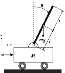
In this section, we test the performance of the proposed adaptive controller on the inverted pendulum system depicted in Fig 1. The dynamic equations of the inverted pendulum system are:

1 2 2 1 , ( ) ( ) ( ), , x x

x f x b x u t

y x = = + = (59) where 2

2 1 1

1

2 1

cos( )sin( ) sin( )

( )

cos ( ) 4

3

mlx x x

g x M m f x m x l M m − + = ⎛ ⎞ − ⎜ ₊ ⎟ ⎝ ⎠ , 1 2 1 cos( ) ( )

cos ( ) 4 3 x M m b x m x l M m + = ⎛ ⎞ − ⎜ ₊ ⎟ ⎝ ⎠ , (60) 1

x = θ is the angular position of the pendulum (see Fig. 1), x₂= θ is the angular velocity of the pendulum. We use_g=_{9.8 m/s}2_{, 1 kgM} = _{is the mass of}

the cart, m=0.1kg is the mass of the pole and l=0.5m is the half length of the pole. The control objective is to make the pole of the pendulum track a sine wave trajectory θ =_m y_m =AMsin( )t with amplitudes AM = π/ 30 during the time interval t∈[0 12.5] s, / 15AM = π during the time interval

[12.5 25] s

t∈ , and finally with amplitude AM =0 as in [1, 3] during the remaining time interval Clearly, the derivatives of the reference y_m exist and are bounded.

The two RBF networks (the first RBF controller and the second RBF estimator) have five radial basis functions. The parameters θ are initialised to 0, and θb are all initialised to 0.5. Other choices have been tried, these last values

[ 2 3− 2 3]. K is chosen as _K=[_{k0 k1}]T =[0.9 5]T_{, and Q in (26) is}

chosen as Q=diag(127,127)>0. Then by solving (26) we can obtain:

376.9078 70.5556

70.5556 26.8111

P= ⎢⎡ ⎤_⎥

⎣ ⎦. (61)

For the first RBF controller, we used γ =10, the input vector x is

composed of two inputs x=[x x_{1 2}] [= θ (K eT − θ_m(2))], the radial basis functions are chosen as Gaussian functions as given by (11), where the corresponding widths for every function is σ=1.32.

For the second RBF estimator, we used α =0.005, the input vector x_b is composed of two inputs the error e and the variation of error de, i.e.,

[ ]

b m m

x = θ − θ θ − θ , the radial basis functions are chosen as Gaussian functions as given by (11), where the corresponding widths for every function is

0.54

b

σ = .

The initial conditions are ( (0),x₁ x₂(0))T = −( 0.2 rad, 0 rad/sec) and the step size is set to dt=0.01. The results of the simulation are shown in Figs. 2 to 6. The system output ( )y t (pole angle) is in continuous while the reference signal y t_m( ) is in dotted.

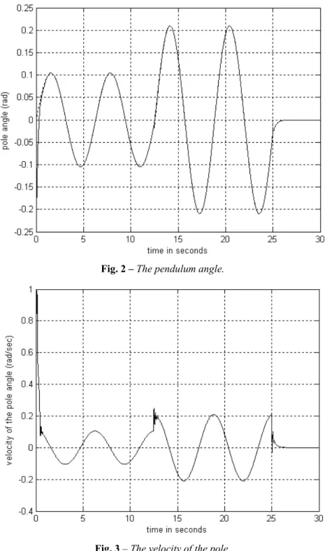
Fig. 2 –The pendulum angle.

Fig. 4 – The tracking error e= θ − θm.

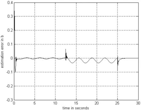
Fig. 6 – The estimation error when estimating ( )b x by the second RBF system.

Fig. 2 shows the response of the pole angle from the initial position ( 0.2,0)− . We can see that the system state x t1( )= θ tracks the desired

trajectory y_m = θ_m very well. Fig. 3 shows the velocity of the pole. Fig. 4. shows that the tracking error is converging very rapidly to a value close to zero. Fig. 5 represents the corresponding control input which peaks at t=12.5 s (because of the first amplitude variation from AM = π/ 30 to AM = π/ 15), and at t=25 s (because of the second amplitude variation from AM = π/ 15 to

0

5 Conclusion

In this paper, we introduced an adaptive controller for a class of unknown nonlinear systems. It is based on two RBF networks: the first network approximates the ideal control law which cannot be implemented because the system dynamics are unknown, the second network estimates the unknown virtual control gain. The centres of the basis functions and the connection weights in the two RBF networks were adjusted on line. The k-means algorithm was used for the centres adjustment. The connection weights of the two RBF networks are adapted according to a law derived using Lyapunov stability theory. The proposed method guarantees the stability of the resulting closed-loop system in the sense that all signals involved are bounded. Finally, we used the proposed approach to control the inverted pendulum system in both tracking and regulation cases. Simulation results showed the good performances of the algorithm.

6 References

[1] X. Ban, X.Z. Gao, X. Huang, A.V. Vasilakos: Stability Analysis of the Simplest Takagi-Sugeno Fuzzy Control System using Circle Criterion, Information Sciences, Vol. 177, No. 20, Oct. 2007, pp. 4387 – 4409.

[2] S. Chen, S.A. Billings, P.M. Grant: Recursive Hybrid Algorithm for Nonlinear Systems Identification using Radial Basis Function Networks, International Journal of Control, Vol. 55, No. 5, May 1992, pp. 1051 – 1070.

[3] P.C. Chen, C.W. Chen, W.L. Chiang: GA-based Modified Adaptive Fuzzy Sliding Mode Controller for Nonlinear Systems, Expert Systems with Applications, Vol. 36, No. 3, April 2009, pp. 5872 – 5879.

[4] T.P. Chen, H. Chen: Approximation Capability to Functions of Several Variables, Nonlinear Functionals and Operators by Radial Basis Function Neural Networks, IEEE Transactions on Neural Networks, Vol. 6, No. 4, July 1995, pp. 904 – 910.

[5] C. Darken, J. Moody: Fast Adaptive k-means Clustering: Some Empirical Results, International Joint Conference on Neural Networks, San Diego, CA , USA, Vol. 2, June 1990, pp. 233 – 238.

[6] K. Funahashi: On the Approximate Realization of Continuous Mappings by Neural Networks, Neural Networks Vol. 2, No. 3, 1989, pp. 183 – 192.

[7] K. Funahashi, Y. Nakamura: Approximation of Dynamical Systems by Continuous Time Recurrent Neural Networks, Neural Networks, Vol. 6, No. 6, 1993, pp. 801 – 806.

[8] S. Haykin: Neural Networks, A Comprehensive Foundation, Prentice Hall, Delhi, India, 1998.

[9] M. Hojati, S. Gazor: Hybrid Adaptive Fuzzy Identification and Control of Nonlinear Systems, IEEE Transactions on Fuzzy Systems, Vol. 10, No. 2, April 2002, pp. 198 – 210.

[11] D.R. Hush, B. Horne: Efficient Algorithms for Function Approximation with Piecewise Linear Sigmoidal Networks, IEEE Transactions on Neural Networks, Vol. 9, No. 6, Nov. 1998, pp. 1129 – 1141.

[12] A. Isidori: Nonlinear Control Systems, Springer, Berlin, Germany, 1995.

[13] R. Marino, P. Tomei: Nonlinear Control Design: Geometric, Adaptive and Robust, Prentice Hall, NJ, USA, 1995.

[14] K.S. Narendra, K. Parthasarathy: Identification and Control of Dynamical Systems using Neural Networks, IEEE Transactions on Neural Networks, Vol. 1, No. 1, March 1990, pp. 4 – 27. [15] R.M. Sanner, J.E. Slotine: Gaussian Networks for Direct Adaptive Control, IEEE

Transactions on Neural Networks, Vol. 3, No. 6, June 1992, pp. 837 – 863.

[16] S.N. Singh, M. Steinberg: Adaptive Control of Feedback Linearizable Nonlinear Systems with Application to Flight Control, Journal of Guidance, Control, and Dynamics, Vol. 19, No. 4, July-Aug. 1996, pp. 871 – 877.

[17] J.E. Slotine, L. Weiping: Applied Nonlinear Control, Prentice Hall, NJ, USA, 1991. [18] S.B. Stojanovic, D.Lj. Debeljkovic, I. Mladenovic: Simple Exponential Stability Criteria of

Linear Discrete Time-Delay Systems, Serbian Journal of Electrical Engineering,Vol. 5, No. 2, Nov. 2008, pp. 191 – 198.

[19] E. Tzirkel-Hancock, F. Fallside: Stable Control of Nonlinear Systems using Neural Networks, International Journal of Robust and Nonlinear Control, Vol. 2, No. 1, May 1992, pp. 63 – 86.

[20] C.H. Wang, H. Liu, T. Lin: Direct Adaptive Fuzzy-neural Control with State Observer and Supervisory Controller for Unknown Nonlinear Dynamical Systems, IEEE Transactions on Fuzzy Systems, Vol. 10, No. 1, Feb. 2002, pp. 39 – 49.