Motherhood and women in the labor market : different behaviors between women with and without children - an evidence for Brazil

(1)

Motherhood and women in the labor market: different behaviors between women with and without children - an evidence for Brazil

Elaine Toldo Pazello∗ Reynaldo Fernandes∗∗

1. Introduction

The growing participation of women in the labor market has been one of the most widely empirically investigated issues. In Brazil, for instance, women’s labor force participation rate showed a 35% increase between 1982 and 1997, and this rate is even higher for younger and better educated women. Since then, several studies have sought to identify the determining factors for women’s new behavior. Higher professional qualification, among other factors, has been pointed out as a key element that has certainly contributed to the greater participation of women in the labor market.1

In a traditional model of individual labor supply, individuals maximize a utility function subject to a budget constraint (the amount spent on goods and services must equal their earnings in the labor market, given the wage-hour) so that they can decide how to allocate their time between work and leisure.2 However, factors that influence this decision may be very different for men and women. Having young children, for example, may be a major limiting factor for the presence of women in the labor market than for the presence of men.

The aim of the present study is to measure the impact motherhood has on women’s participation in the labor market. Understanding this relationship is important for various reasons. Firstly, the relationship between children and engagement may help explain the greater participation of women in the labor market from the 1950s onwards: having fewer children3 would be related to greater labor market participation. Secondly, the role of motherhood in women’s engagement in the labor market might be one of the factors underlying the differences in wage and occupations between men and women, an issue that has not been well documented in the literature yet. Also, the interest in the

∗

University of São Paulo - Brazil. ∗∗

University of São Paulo - Brazil.

1

For a survey of empirical studies on women’s labor supply, see Killingsworth and Heckman (1986). In Brazil, see Scorzafave and Menezes-Filho (2001), Soares and Izaki (2002), among others.

2

Leisure includes all activities outside the labor market, such as home-based work.

3

(2)

relationship between having children and engagement has been growing due to the increasing number of models that relate family to labor market, in which the link between mother’s participation and the number of children is noticeable.4

According to the economic theory, the impact of motherhood on women’s labor supply could be defined as the net result of income and substitution effects that follow childbirth. The per capita household income decreases when a child is born. Thus, the income effect would be positive on the women’s participation in the labor market. The

substitution effect, though, is directly related to the mother’s opportunity cost.

Depending on the wages women get in the labor market, they may prefer to exchange work outside the home for household activities, including taking care of the children. In this case, the substitution effect would be negative.5 Conversely, using Becker’s model (1965), the higher the income, the higher the relative cost of time and of time-intensive goods. Considering that taking care of the children is time-intensive, women would supposedly want to have fewer children.6 In general, it is believed that the substitution effect stands out, which means that motherhood has a negative effect on women’s labor supply.

However, measuring the impact of motherhood on women’s engagement is not an easy task. The endogeneity in the children/engagement relationship does not allow comparing the behavior of women with children to that of women without children. In addition to the simultaneity of both events (having children and working), different women may have different preferences regarding children and work. Therefore, some women would rather have children than work while others would rather work than have children. The comparison between these groups would imply a negative relationship between fertility and labor supply, even without any causal effect of children on engagement. In the first studies about the relationship between fertility and women’s labor supply, according to the economical approach, the number of children was an explanatory factor for women’s labor supply. On the other hand, in demographical study, wage or any other measure of women’s labor supply would play a determining

4

Children’s age composition in the family, for instance, may influence the additional worker’s estimates (added work effect).

5

Mincer (1963) was the first author to derive the negative relationship between the mother’s opportunity cost (measured by the wage rate) and fertility.

6

(3)

role in fertility. This is clear evidence that any causal analysis between fertility and engagement should be undertaken with caution.

Instrumental variable analysis7 is a widely used method for addressing the endogeneity of fertility in the equations for women’s participation in the labor market. Nevertheless, finding “instruments” for the study of fertility that are exogenous and have a high explanatory power is not an easy task. Some instruments, such as religion, ethnic group, mother’s number of siblings, mother’s opinion about the ideal family size and duration of marriage, are correlated with fertility, but it is difficult to prove they would not have any effect on the behavior of women in the labor market other than through fertility.

There are several seminal works dealing with this issue, among which are the studies conducted by Rozenzweig and Wolpin (1980), Bronars and Grogger (1994) and Gangadharan and Rosenbloom (1996), in which twin births are regarded as an exogenous variation in fertility; or the works by Angrist and Evans (1988) and Iacovou (2001), who use parents’ preferences for balanced families in terms of the sex of their children (“one boy and one girl”) as an instrument for the number of children.

The aim of this paper is to assess the impact motherhood has on women’s labor market variables, by specifically comparing women with and without children. As in the works cited previously, we make use of an instrument to deal with the endogeneity of the children-engagement relationship. We use the occurrence of stillbirths. The idea is to compare women with at least one child with others who do not have any, but who have experienced a stillbirth (i.e., tried to have a child but were not able to). The hypothesis is that both women have ex-ante similar preferences, since both got pregnant, which means that both wanted to have children. Iacovou (2001) highlights the potentiality of this type of instruments, that is, instruments related to fertility problems, which are not commonly used, due to the rarity of these events.

One may argue that the occurrence of stillbirths is correlated with income and, in this case, that the instrument used would not actually be exogenous. Nevertheless, as will be discussed further ahead, the observable characteristics that determine income will be controlled. On top of that, it should be underscored that the results obtained will be “mean results”. The fact that the information regarding the date of stillbirth is not known does not allow distinguishing short-term impacts – which in this case would be

7

(4)

the results of the comparison of labor force participation between women who have had a baby recently and those who have lost their baby recently – from long-term ones. This study contributes to the relevant literature in two different ways: first, by proposing a new instrument for the assessment of fertility variables, since occurrence of stillbirth, to the best of our knowledge, has not been described in the literature yet; secondly, by evaluating the effect of motherhood on women’s participation in the labor market, comparing women with and without children, something that has not yet been investigated. In most articles, comparisons are made among women with children.8

After this introduction, the paper is organized into four more sections. Section 2 describes the data used in the empirical exercise. Section 3 discusses the methodology used. Section 4 describes the obtained results, and section 5 concludes.

2. Data

PNAD (National Household Sample Survey) data provided by IBGE (Brazilian Institute of Geography and Statistics) for years 1992 to 1999 were used. In the PNAD, there is a specific chapter about fertility, whose questions are answered by all resident women aged 15 or older. The occurrence of stillbirth is one of the topics investigated in this chapter. The interviewees should answer the following question: “Until 09/25/XX (third week of September of the reference year), did you give birth to a stillborn baby at the seventh month of pregnancy or later? All women who answered ‘yes’ and who had not had a live birth were included in the treatmentgroup, whereas all the women who answered ‘no’ and who had already had at least one live birth were included in the control group.

The fact that pregnancy reached seven months or more differentiates stillbirth from induced abortion, corroborating the hypothesis proposed herein that the women

8

(5)

wanted to have their child (at least after getting pregnant). It is implicitly assumed that unwanted pregnancy is randomly distributed across groups.

At first, all Brazilian women living in urban areas who met any of the two criteria described above were included in the study. In the case of women in the control group, in order to make sure that the family member identified as being the child was actually the child of the couple, or of the household head when the spouse was absent, we excluded cases in which the age difference between the mother and the oldest child was less than 14 or greater than 45 years. All women aged between 15 and 52 were included. The selection of 52 years as the upper age limit is due to the aim of this study to evaluate the impact of motherhood on women’s participation in the labor market.

Women who had given birth to a stillborn child, but who had children, were excluded from the analysis, since the objective is to associate stillbirth with problems related to women’s fertility. On the other hand, young women who had given birth to a stillborn child, but are possibly able to have children, were erroneously included in the treatment group. For that reason, in order to provide robustness to the analysis, part of the empirical exercises will be carried out initially with all women aged between 15 and 52, and subsequently, only with a sample of women aged between 40 and 52.

Additionally, two control groups were established: one considering all women with at least one child and the other one considering only those who had one child. The objective is to evaluate whether the impact of motherhood on engagement varies with the number of children. If time spent on taking care of the children does not vary significantly with the number of children, the impact of motherhood on engagement should be similar in both groups. This differentiation between control groups will only be considered for the main group, which includes women aged between 15 and 52.

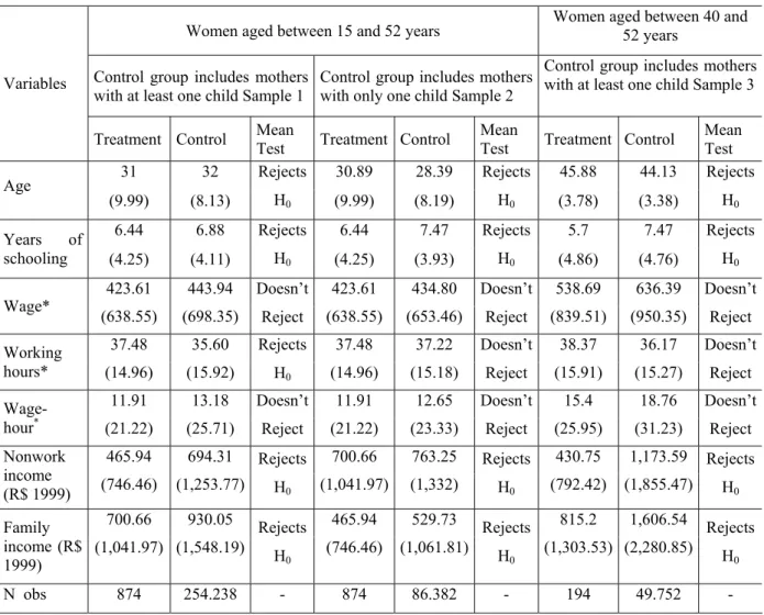
The following table presents some descriptive characteristics of both treatment and control groups. Only in sample 1 estimates, the t test revealed a negative age difference between women in the treatment group and those in the control group. For the other samples, such difference was significantly positive. This result indicates that young women might be being included in the treatment group. As also expected, women in the control group, regardless of the sample, are better educated, have a higher family income and a higher nonwork income.9 This is strong evidence that stillbirth is associated with poverty. As to specific labor market characteristics, a difference in

9

(6)

behavior is observed only in sample 1 for the working hours variable. In this case, women in the treatment group have longer working hours than women in the control group.

Table 1: Description of observable characteristics of the groups (Means for the 1992-1999 period)

Women aged between 15 and 52 years Women aged between 40 and _{52 years}

Control group includes mothers with at least one child Sample 1

Control group includes mothers with only one child Sample 2

Control group includes mothers with at least one child Sample 3 Variables

Treatment Control Mean

Test Treatment Control

Mean

Test Treatment Control

Mean Test

31 32 30.89 28.39 45.88 44.13

Age

(9.99) (8.13) Rejects

H0 (9.99) (8.19)

Rejects

H0 (3.78) (3.38)

Rejects H0

6.44 6.88 6.44 7.47 5.7 7.47

Years of

schooling (4.25) (4.11) Rejects

H0 (4.25) (3.93)

Rejects

H0 (4.86) (4.76)

Rejects H0

423.61 443.94 423.61 434.80 538.69 636.39

Wage*

(638.55) (698.35) Doesn’t

Reject (638.55) (653.46) Doesn’t

Reject (839.51) (950.35) Doesn’t

Reject

37.48 35.60 37.48 37.22 38.37 36.17

Working

hours* (14.96) (15.92) Rejects

H0 (14.96) (15.18)

Doesn’t

Reject (15.91) (15.27) Doesn’t

Reject

11.91 13.18 11.91 12.65 15.4 18.76

Wage-hour*

(21.22) (25.71) Doesn’t

Reject

465.94 694.31 700.66 763.25 430.75 1,173.59

Nonwork income

(R$ 1999) (746.46) (1,253.77) Rejects

H0 (1,041.97) (1,332)

Rejects

H0 (792.42) (1,855.47)

Rejects H0

700.66 930.05 465.94 529.73 815.2 1,606.54

Family income (R$ 1999)

(1,041.97) (1,548.19) Rejects

H0 (746.46) (1,061.81)

Rejects

H0 (1,303.53) (2,280.85)

Rejects H0

N obs 874 254.238 - 874 86.382 - 194 49.752 -

* For these variables, the number of observation is smaller than that on the last line, since only employed women answer these questions.

Two-tailed t tests were used for the mean differences between independent samples, considering

dissimilar variances, where h0: treatment – control=0. The level of confidence considered for rejection

is 10%.

Treatment group= women without children who gave birth to at least one stillborn child.

Control group= women with at least one child (or women with only one child) who have never given birth to a stillborn child.

Standard deviation is shown in brackets.

(7)

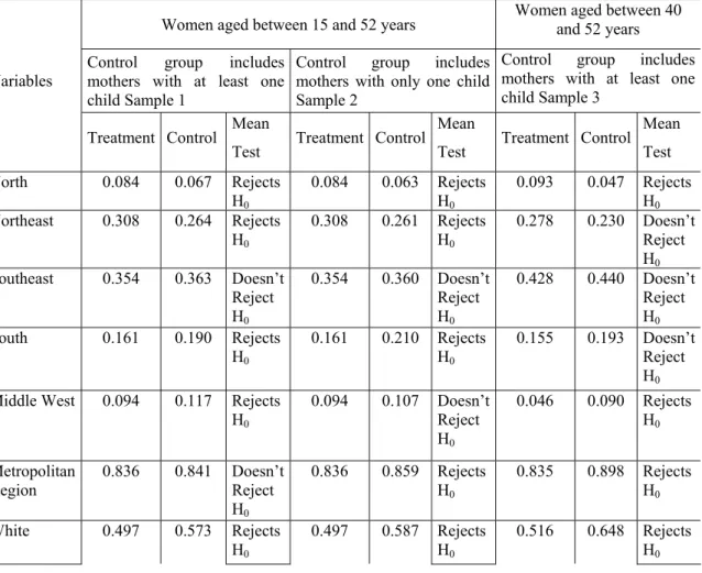
differences results only to four variables, namely: dummy variable for the north region; dummy variable for the southeast region; dummy variable for white women and dummy variable for activity status.

Estimates suggest an overrepresentation of women in the treatment group for the north region, which could be explained by the fact that this region is less developed than the others in terms of healthcare services for women, such as prenatal care, birth control services, etc. This result is one more piece of evidence of how important the control of women’s income is for the estimates being made. The greater proportion of non-white women in the treatment group is another piece of evidence that stillbirth may be correlated with poverty. The fact that women in the treatment group have a bigger representativeness in the EAP indicates a possible negative effect of motherhood on participation. Obviously, such difference might be capturing other elements than the presence of children.

Table 2: Distribution of groups according to region, race, marital status and participation in the labor market.

Women aged between 15 and 52 years Women aged between 40 _{and 52 years}

Control group includes mothers with only one child Sample 2

Variables

Treatment Control Mean

Test Treatment Control Mean

Test Treatment Control Mean Test North 0.084 0.067 Rejects

H0

0.084 0.063 Rejects H0

0.093 0.047 Rejects H0

Northeast 0.308 0.264 Rejects H0

0.308 0.261 Rejects H0

0.278 0.230 Doesn’t Reject H0

Southeast 0.354 0.363 Doesn’t Reject H0

South 0.161 0.190 Rejects H0

0.161 0.210 Rejects H0

Middle West 0.094 0.117 Rejects H0

0.046 0.090 Rejects H0

Metropolitan Region

0.836 0.859 Rejects H0

0.835 0.898 Rejects H0

White 0.497 0.573 Rejects H0

0.497 0.587 Rejects H0

(8)

Present Spouse

0.831 0.726 Rejects H0

0.722 0.799 Rejects H0

Active 0.654 0.579 Rejects H0

0.654 0.591 Rejects H0

0.696 0.620 Rejects H0

Occupied* 0.876 0.905 Rejects H0

Number of observations

874 254.238 - 874 86.382 - 194 49.752 -

* For these variables, the number of observations is smaller than that on the last line, since it concerns only women who belong to the EAP.

Difference of proportion tests were performed, where h0: treatment – control=0. The level of

confidence considered for rejection is 10%.

Treatment group= women without children who gave birth to at least one stillborn child.

Control group= women with at least one child (or women with only one child) who have never given birth to a stillborn child.

Considering the dummy for marital status, while in the first two samples there is a greater proportion of married women in the treatment group (although this result is statistically significant only for sample 2), the opposite occurs in sample 3, that is, there is a greater proportion of married women in the control group. Very likely, this apparent contradiction is related to how both treatment and control groups were structured. As previously discussed, it could be that young married women have not succeeded in their first attempts to become mothers, which does not mean they will not succeed in the future. That would explain the greater proportion of married women in the treatment group. On the other hand, when a sample is limited only to older women, this difference should not exist. But, this is actually the inverse. Several factors can explain such result. A possible explanation could be the positive correlation between stillbirth and poverty. The fact that family stability is inversely related to poverty could explain this inversion.

3. Methodology

As proposed in the introduction, the aim of this paper is to measure the impact of fertility on women’s participation in the labor market. Specifically, it is an attempt to investigate the differences in labor market behavior of women with and without children. The estimates focus on three variables related to the labor market: labor market participation, working hours and wage per hour. Before introducing the statistical procedures, it is important to discuss the identification strategy adopted.

(9)

The identification strategy used in this paper consists in comparing women with children to those without children who have given birth to a stillborn child. The fact that women without children gave birth to at least one stillborn child may be interpreted as an indicative sign that they wanted to have a child but, for physical or medical reasons, they were not able to. It is possible that a woman’s preference for children changes after she gives birth to a stillborn child. However, hypothetically, such preference was probably similar to that of a woman who gave birth to a live-born infant. This solves the endogeneity of the decision to have children.10

In other words, the occurrence of stillbirth is used as a proxy for fertility problems, and that is why, of all women who gave birth to a stillborn child, we selected only those who said they had never had a live birth.

The problem with this identification strategy is that stillbirth is very likely to be correlated with poverty, as pointed out in the descriptive analysis presented in the previous section. Less educated and usually poorer women do not have an adequate medical follow-up during pregnancy, either because they cannot afford it or due to lack of information, which ends up increasing their probability of giving birth to a stillborn infant. This means that stillbirth does not solve the endogeneity inherent to the children-engagement relationship.

Nevertheless, if stillbirth is correlated only with the observed variables that determine income (such as level of education, age, region etc.), the solution is simple: all you have to do is to condicionate women’s participation in the labor market on these variables. That is, the hypothesis is that by considering a set of observable characteristics X and by considering that both women have the same preferences regarding children (since both got pregnant), the process that determines which of them has a child or not is random.

3.2 Statistical procedures

Initially, women were divided into two different groups: those without children who gave birth to a stillborn child and those with at least one child who have never

10

(10)

given birth to a stillborn child. Alternatively, as already mentioned, a control group was established including women with only one child and who have never given birth to stillborn child. Let Y be the dependent variable of interest (participation, working hours or wage per hour), we may estimate that:

ε β

β

α + + +

=

∑

= i

i iX

treat Y

26

2

1 (1)

where treat is a dummy variable with value 1 if the woman belongs to the treatment group, that is, without children (treat). The covariate matrix includes the following variables: woman’s current age (age), woman’s squared age (age2), years of schooling (educ), a dummy variable with value 1 if the woman is married (married), a dummy variable with value 1 if the woman lives in a metropolitan region (metrop), four dummy variables indicating the macro-regions, having the southeast as the reference region (d_macroi) and six dummy variables for control of PNAD years, having 1999 as the

reference year (d_yeari). When Y is the probability of participation, we regard it as

being described by a logistic function.

The coefficient of interest is that of the treat variable: a positive value for this coefficient indicates that women without children have, conditional on X, a higher probability to participate in the labor market, longer working hours or higher wages.

It is interesting to observe that the empirical exercise does not work with stillbirth as an instrument, that is, the treat dummy variable is directly included in the equations, as described in (1). When that is done, the effect obtained is that of the total number of children. If the treat variable were used as an instrument for the number of children variable, the effect obtained would be “per child.”11 By restricting the control group only to women with at least one child who have not given birth to a stillborn child, the possibility to work with instrumental variables was lost. However, this choice was not arbitrary. A way to be sure that women in the control group were fertile was exactly the presence of children.12

11

As shown in Angrist and Krieger (1999), the coefficient that show the impact of the instrumentalized number of children on wage, for example, is the ratio between βLS from the equation in which wage is the dependent variable and βLS from the equation in which number of children is the dependent variable.

12

(11)

In the equations for working hours and wage per hour, the marginal effect of the “presence of children” can be obtained by the coefficient of the treat variable. However, for the participation equation this effect is not directly obtained. In this case, the “average effect of the treatment on the treated” was calculated.

As for the analysis of labor market variables – working hours and market wages – there is an additional difficulty. For the probability of participation, all women of the sample are included in the estimation. Nevertheless, for the working hours and wage per hour variables, only those women who have positive working hours and/or payment will be included in the estimates, which means only part of women without children and part of women with children. That is, there is a selection in both groups. In order to correct this possible selection bias, we used the process of estimation proposed by Heckman. The variable used for the selection is the nonwork income. Hypothetically, such income would not be correlated with the unobservable variables that determine women’s working hours and wages in the labor market, but with their participation, since the higher the income, the less necessary the income obtained by women in the labor market and, therefore, the lower probability of women’s participation in the labor market.13

The variables included in the estimate of the selection equation were: age, age2, educ, married, metrop, d_macro, d_year, nonwork, d_decil and treat. The variables included in the main equation (the dependent variables are the variables of interest, i.e., working hours and wage per hour) were the same ones included in the estimate of the selection equation, except for nonwork income (nonwork, d_decil).

3.3 The matching procedure

In order to provide robustness to the results, a matching procedure was carried out. By definition, matching consists in pairing units from different groups that are similar in terms of observable characteristics. This procedure has gained some importance in the literature after being used in the evaluation of training programs.14

The aim here was to find for each childless woman who gave birth to at least one stillborn child (i.e.: each woman in the treatment group) a woman who could represent

13

The use of the nonwork income as instrument is more appropriate when applied to wage per hour than to the working hours. One might think that a higher nonwork income would make women work fewer hours.

14

(12)

her in the situation of having given birth to a live-born baby. So, the idea was to select a subsample of the control group, consisting of women who were “exactly” identical (in observables) to the women in the treatment group, except for the fact that women in the treatment group do not have children and the women in this subsample do. The econometric exercises described in the previous subsection are estimated for this new set of women resulting from the matching. The objective is to provide robust results, since the main difference between OLS and matching estimates lies in the weighting process. The identification hypothesis remains the same.15

As in this empirical exercise the dimensionality of the covariate vector is quite large, propensity score matching was used, consisting in pairing units based on the propensity score.16 Initially, each woman was estimated to have a probability to belong to the treatment group, which means a probability not to have children but to give birth to a stillborn child. Based on this estimate, a woman in the control group with the same propensity score was chosen for each woman in the treatment group. However, it is not always possible to find units with the same propensity score. In this case, women with very similar propensity scores were matched/paired. This procedure is described in the literature as “k-nearest-neighbors matching.”.

At first, the researcher can choose as many “neighbors” as he pleases, and he can even use the whole sample. In the latter case, based on a specific distance measure, different weights would be given to the non-treated units, depending on their distance from the treated unit.17 When using only one neighbor, weight 1 is being implicitly given to the nearest observation and weight zero to the remaining ones. In the procedure adopted here 1, 5 and 10 neighbors were chosen. In all cases, we chose: i) a maximum distance between the units, that is, the difference of propensity scores between the treated and the selected control units could not be greater than 0.0001;18 ii) common support, that is, maximum and minimum propensity score values are the same for the groups. Furthermore, the procedures were carried out without replacement, meaning that each control unit could be paired only once.

For the estimation of the propensity score, we admitted that the probability of woman i belonging to the treatment group followed a logistic function, in which the

15

Angrist and Krueger (1999)

16

Rosenbaum and Rubin (1983) show that, if conditional on X, the “separation” of individuals into treatment and control groups occurs at random, so conditional on P(X) – that is, on the propensity score – such separation is still random.

17

Heckman, Ichimura and Todd (1997), Heckman, Ichimura and Todd (1998)

18

(13)

vector of regression (X) was the same as the one in equation (1), as previously described, with some additional interactions. An important observation should be made at this point.

One way to verify matching accuracy consists in estimating the same propensity score equation in the sample resulting from the matching. If the matching was successful, the covariates will lose their explanatory power. However, the most parsimonious form of equation (1) was not capable of eliminating the differences observed between the groups. Specifically, after the matching, there still were significant differences in the age and marital status variables. For this reason, as suggested in Dehejia and Wahba (1998), additional interactions among the variables were included in the propensity score equation. The following interactions were used: (age*married), (age2*married), (educ*age), (educ*age2), (age*d_macro), (age2*d_macro), (married *d_year) and (educ*d_year).

As mentioned, the same previously described econometric exercises were carried out for the paired samples (that is, for the subsamples obtained from the matchings). As presented in section two, three different samples are used, namely:

• Sample 1= includes all women aged between 15 and 52 years and whose control group is formed by all women with no stillbirths and who have at least one child.

• Sample 2 = includes all women aged between 15 and 52 years whose control group is formed by all women with no stillbirths and with only one child.

• Sample 3= includes all women aged between 40 and 52 years whose control group is formed by all women with no stillbirths and with at least one child.

For each sample, the matching procedures produced three subsamples, whose sizes depend on the number of “neighbors” included. This means producing nine estimates of the possible effect of motherhood for each variable of interest. In addition to these nine estimates, there obviously are those derived from the original samples; therefore, twelve estimates.

(14)

not be necessary. This procedure is, in fact, a different way to check whether the composition of the control group is balanced, that is, if the matching was successful. If successful, the differences in the estimated impact of motherhood on the dependent variables of interest should not vary among the estimates with and without covariates. This procedure is known as adjusted matching. Estimates with and without control will be presented.

4. Results

The logit equations that were used as a base for the calculation of the propensity scores used in the matchings are not presented in the text for space reasons. These same equations were estimated for the paired samples as a way to evaluate matching success. However, also due to space reason, they are not presented in the text. It is worth mentioning, though, that in the paired samples, in all cases, Wald test statistics indicated that it is not possible to reject the null hypothesis that all coefficients togetherare equal to zero. Some evidence that matching was successful.

(15)

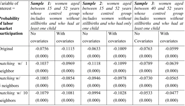
Table 3: Impact of the presence of children on the probability of labor market participation

Sample 1: women aged between 15 and 52 years whose control group includes women without stillbirths and who had at least one child

Sample 2: women aged between 15 and 52 years whose control group includes women without stillbirths and who had only one child

Sample 3: women aged between 40 and 52 years whose control group includes women without stillbirths and who had at least one child

Variable of interest = Probability of labor market

participation No covariates With covariates No covariates With covariates No Covariates With covariates -0.0756 -0.1115 -0.0633 -0.1009 -0.0763 -0.0599 Original

(0.000) (0.000) (0.000) (0.000) (0.000) (0.000) -0.1037 -0.0969 -0.1118 -0.1099 -0.0789 -0.0639

matching w/ 1

neighbor (0.000) (0.000) (0.000) (0.000) (0.000) (0.000) -0.1003 -0.0854 -0.0946 -0.0978 -0.0730 -0.0565

matching w/

5 neighbors (0.000) (0.000) (0.000) (0.000) (0.000) (0.000) -0.1079 -0.1081 -0.0994 -0.1028 -0.0533 -0.0477

matching w/ 10

neighbors (0.000) (0.000) (0.000) (0.000) (0.000) (0.000)

First of all, it is important to highlight that the first value (‘original + no covariates’) for all samples is certainly biased: it is the gross difference of the probabilities of activity between groups, without any control. As shown in the descriptive section, groups are heterogeneous and this result capture different elements other than motherhood that affect participation. In Table 2, shown in the descriptive section, the difference in participation rates between groups would have the exact value presented here.

The analysis of Table 3 shows the existence of a negative impact of motherhood on women’s participation in the labor market. Considering only the estimates when covariates are included, the probability of childless women of being active would fall, on average, -0.1005, -0.1028 and –0.0570 percentage points, respectively, for samples 1, 2 and 3, if they had children. That is, in the first sample, the mean probability of childless women’s participation in the labor force would fall from 65.73% to 55.68% in case they had children. In sample 2, it would go from 65.60% to 55.32% and, in sample 3, from 70.29% to 64.59%.

(16)

found in sample 3. Sample 3 may be capturing a longer-term effect of motherhood, if we consider that women usually want to have children before the age of 40. Thus, in the long-term, although there still exists a difference in the labor market participation of women with and without children, this difference is certainly smaller. An interesting aspect is the higher mean participation of women in this group. By including only women aged 40 years or older, we automatically excluded a large number of younger women who were still in the process of acquiring qualification, who did not participate in the labor market.

Notice that the results, with or without covariates, are quite similar in the paired samples, indicating that the matchings were successful. The largest deviation was that of estimates in sample 3, in which five “neighbors” are considered. In this case, there is a difference of impact around 0.0165 towards the estimate with no control. Due to the consistent results, only the estimates obtained when the covariates are included in the equations were presented for the following variables of interest. Note that results change slightly when 1, 5 or 10 “neighbors” are considered.

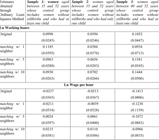
Tables 4 and 5 show the estimated impact of motherhood on working hours and wage per hour.19 Table 4 describes the results obtained through the ordinary least squares method and Table 5 shows those results obtained though the Heckman procedure.

19

(17)

Table 4: Effect of the presence of children on working hours and wage per hour

Ordinary Least Squares Estimates

obtained through

Ordinary Least Squares Method

Sample 1: women aged between 15 and 52 years whose control group includes women without stillbirths and who had at least one child

Sample 3: women aged between 40 and 52 years whose control group includes women without stillbirths and who had at least one child

Ln Working hours

0.0998 0.0594 0.1052 Original

(0.0245) (0.0246) (0.0447) 0.1185 0.0304 0.0934

matching w/ 1 neighbor

(0.0395) (0.0376) (0.0713) 0.0963 0.0656 0.1581

matching w/ 5 neighbors

(0.0280) (0.0283) (0.0545) 0.0930 0.0702 0.1444

(0.0263) (0.0266) (0.0506)

Ln Wage per hour

-0.0237 -0.0213 -0.1413 Original

(0.0365) (0.0367) (0.0806) -0.0211 -0.0039 -0.1238

(0.0534) (0.0528) (0.1159) 0.0024 0.0061 -0.1072

(0.0397) (0.0400) (0.0883) 0.0215 0.0110 -0.0966

(0.0381) (0.0386) (0.0835) Significant standard deviation in brackets

With regard to working hours, the results obtained, in almost all cases, using either OLS or Heckman’s method,20 indicate that childless women work longer. The magnitude of the coefficient, however, differs between the samples. Moreover, for the same sample, the magnitude of the coefficient differs between the subsamples resulting from the matchings. Focusing the attention on the estimates by using Heckman procedure, the mean coefficient for sample 1 was around 0.126, for sample 2, 0.07 and for sample 3, 0.147. Given that the coefficient associated with the dummy treat can be seen as the logarithm of the ratio of working hours of women with and without children, the antilog of this coefficient is exactly the difference between women’s working hours. According to this calculation, we can observe that childless women have, on average, working

20

(18)

hours around 13%, 7% and 16% longer than those estimated for women with children, respectively, in samples 1,2 and 3.

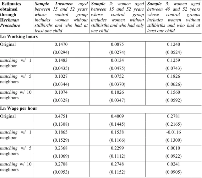
Table 5: Effect of the presence of children on working hours and wage per hour

Heckman Procedure Estimates obtained through Heckman Procedure

Sample 1:women aged between 15 and 52 years whose control group includes women without stillbirths and who had at least one child

Sample 3: women aged between 40 and 52 years whose control groups includes women without stillbirths and who had at least one child

Ln Working hours

0.1470 0.0875 0.1240 Original

(0.0294) (0.0274) (0.0524) 0.1483 0.0134 0.1259

(0.0435) (0.0475) (0.0743) 0.1027 0.0752 0.1826

(0.0344) (0.0370) (0.0626) 0.1074 0.1026 0.1560

(0.0328) (0.0347) (0.0592)

Ln Wage per hour

0.4751 0.4009 0.2781 Original

(0.1308) (0.1445) (0.2165) 0.1865 0.1538 -0.0116

(0.1529) (0.1166) (0.1300) 0.2368 0.2299 0.0010

(0.1069) (0.1112) (0.0922) 0.2708 0.2748 0.0241

(0.0953) (0.1152) (0.0905)

Standard deviation in brackets

(19)

When the wage per hour is the variable of interest, some aspects should be underscored. The first one is that the discrepancy of estimates across samples and, in a sample, across the subsamples obtained from the matching, is higher if compared to the other variables that have already been analyzed. Secondly, none of the coefficients obtained through OLS is statistically significant. However, the same does not apply to the estimates obtained through the Heckman procedure. Finally, the coefficients obtained from the original database are always higher if compared to the ones obtained from the paired samples, even though the standard deviations are similar.

Focusing some attention on the estimates obtained through the Heckman procedure, it is interesting to note that, in sample 3, no coefficient was statistically significant, not even when the estimates were obtained from the original database. This means that, in the long-term period, even if childless women work longer, the wage per hour rate obtained by them does not differ from the one obtained by the women with children. This finding shows that withdrawal from the labor market because of motherhood does not seem to influence future earnings.

In samples 1 and 2, coefficients are significant when the estimates are obtained from the original database or from the paired samples when 5 or 10 “neighbors” are considered, but the magnitude of the former is at least 46% higher. Working with this mean impact and using the antilog again, we can see that childless women get wages 39% and 35% higher when compared to women with children, respectively, in samples 1 and 2. One possible explanation for this result can be found in the argument of the theory of compensating wage differentials (CWD) used to explain the wage gaps between men and women. In order to reconcile childcare and work activities, women with children would accept jobs with more flexible and/or shorter working hours (as pointed out by the herein), which usually pay less.

(20)

their productivity difference is high compared to those of women who remained in the labor market, but it tends to disappear with time.

4. Final remarks

This paper aimed at measuring the impact of motherhood on women’s participation in the labor market, by comparing women with and without children. Because of the existing endogeneity in the children-engagement relationship this is not an easy task. In this paper, stillbirth was explored as an identification strategy. In order to provide robustness to the estimates, both traditional and matching methods are used.

The results obtained pointed out to the existence of a negative impact of motherhood on women’s participation in the labor market. This impact does not seem to vary as much as the number of children and tends to diminish in the long run. As for the working hours, we can observe that women without children work longer than women with children. The magnitude of such difference, however, varies according to the number of children and is higher in the long run, as opposed to participation.

At last, as for the wage per hour, the results (using Heckman procedure) indicated that, in the long run, the wage per hour rate obtained by women without children does not seem to differ from the one obtained by women with children, probably showing that withdrawal from the labor market because of motherhood has no effect on future income. Nevertheless, in samples 1 and 2, in which women aged between 15 and 52 years are included and, for this reason, produce the mean impact on the variables of interest, the results point towards the existence of a wage gap in favor of women without children. It is possible that, in order to reconcile childcare and work activities, women with children may accept lower wages per hour providing that the job offers more flexible and/or shorter working hours.

(21)

(22)

References

ANGRIST, J. D. and EVANS, W. N. Children and Their Parents’ Labor Supply: Evidence from Exogenous Variation in Family Size. The American Economic Review, vol.88, nº 3, 1998.

ANGRIST, J. and KRUEGER, A. Empirical strategies in labor economics. In: ASHENFELTER, O. and CARD, D.. Handbook of Labor Economics, vol. 3A. Elsevier, 1999.

BECKER, G.. A theory of the allocation of time. Economic Journal, 75, 1965.

BRONARS, S. G. and GROGGER, J. The Economic Consequences of Unwed Motherhood: Using Twin Births as a Natural Experiment. The American Economic Review, vol. 84, nº 5, 1994.

DEHEJIA, R.H. and WAHBA, S. Propensity score matching methods for non-experimental studies causal studies. NBER Working Paper Series, n. 6829.Cambridge, 1998.

GANGADHARAN, J. and ROSENBLOOM, J. L. The effects of child-bearing on married women’s labor supply and earnings: using twin births as a natural experiment. NBER Working Paper Series, nº 5647. Cambridge, MA, 1996.

HECKMAN, J., ICHIMURA, H. and TODD, P. Matching as an econometric evaluation estimator. The Review of Economic Studies, 65, 1998.

HECKMAN, J., ICHIMURA, H. and TODD, P. Matching as an econometric evaluation Estimator: evidence from evaluating a job training programme. The Review of Economic Studies, 64, 1997.

IACOVOU, M. Fertility and female labour supply. ISER Working Papers, nº. 19, UK, 2001.

KILLINGSWORTH, M. R. and HECKMAN, J. J. Female Labor Supply: A Survey, in Orley Ashenfelter and Richard Layard , eds., Handbook of Labor Economics, vol. 1, 1986.

ROSEMBAUM, P. E RUBIN, D. The Central Role of the Propensity Score in Observational Studies for Causal Effects, Biometrika, vol. 70, 1983.

RIOS-NETO, E. L. G. O impacto das crianças sobre a participação feminina na PEA: o caso das mulheres casadas urbanas. In: X Encontro Nacional de Estudos Populacionais, Belo Horizonte: ABEP, 1996.

(23)

SCORZAFAVE, L. G. e MENEZES-FILHO, N. A. Participação feminina no mercado de trabalho brasileiro: evolução e determinantes. Pesquisa e Planejamento Econômico, v.31, n.3, p.441-478. Rio de Janeiro, 2001.

SOARES, S. e IZAKI, R. S. A participação feminina no mercado de trabalho. Texto para Discussão do IPEA, n. 293. Rio de Janeiro, 2002.