Demand and supply: price elasticities and corporate performance in the UK

... #'"FUNDAÇÃO ... GETULIO VARGAS EPGE

Escola de Pós-Graduação em Economia

- -

-SEMINÁRIOS

DE PESQUISA

ECONÔMICA

, "Demand and Supply: Price,

Elasticities and Corporate

Performance in the UK."

ProfO Naércio Aquino Menezes Filho

(USP)

LOCAL

Fundação Getulio Vargas

Praia de Botafogo, 190 - 10° andar - Auditório

DATA

30/04/98 (53 feira)

HORÁRIO

16:00h

Demand and Supply: Price Elasticities and

Corporate Performance in the UK

N aercio A. Menezes-Filho

University College London and

Centre for Economic Performance - London School of Economics

Houghton Street, London, WC2A 2AE, UK

e-mail: n.menezes-filho@lse.ac.uk

May 30, 1998

Abstract

This paper investigates the relationship between consumer demand and cor-porate performance in several consumer industries in the UK, using two indepen-dent datasets. It uses data on consumer expenditures and the retail price index to estimate Almost Ideal Demand Systems on micro-data and compute time-varying price elasticities of demand for disaggregated commodity groups. Then, it matches the product definitions to the Standard Industry Classification and uses the estimated elasticities to investigate the impact of consumer behaviour on firm-level profitability equations. The time-varying household characteristics are ideal instruments for the demand effects in the firms' supply equation. The paper concludes that demand elasticities have a significant and tangible impact on the profitability of UK firms and that this impact can shed some light on the relationship between market structure and economic performance.

Keywords: industry studies, profitability, consumer behaviour, identifica-tion, firm-level data.

JEL Classification: LI

The interaction between demand and supply is the cornerstone of economics. In-deed, most models in many different areas of economics need demand concepts to predict the outcome of the analysis. In many cases the price elasticity of demand is the summary measure of consumer behavior used to examine the results of firms' and workers' actions1 • Nevertheless, when it comes to empirical modelling, it is rare to find cross-industry studies that actually use estimated demand elasticities in order to test the predictions of these models. In the opposite spectrum, demand elasticities are usually estimated in order to examine a completely different set of issues, such as taxation and welfare economics2•

This state of affairs is probably due to the difficulty involved in obtaining reliable price elasticities for various products at the appropriate leveI of aggregation and in re-solving the simultaneity problem inherent to any procedure that combines supply and demando This paper aims at starting to fill this lacuna, by combining two completely different data sets, one with data on firms operating in several consumer industries and the other with an unusual richness of information on household characteristics and expenditures on a variety of products, to examine the interaction between demand and supply in the determination of firms' mark-ups.

The recent literature in this area has concentrated on case studies, reflecting a general tendency in the industrial organization field (see Goldberg, 1995, Berry

et

aZ, 1995 and Nevo, 1997). However, it is our opinion that cross-sectional comparison between industries remains interesting and informative, particularly with the advent of panel data, where companies can be followed through time so that firm and industry specific effects can be controlled for. Moreover, the case studies, by restricting the consumer choice to different varieties of just one product (plus sometimes an 'outside good'), have to severely restrict the pattern of substitutability between goods in the demand side. Finally, both the methodology and the results are not generalizable to other industries.

On the other hand, the vast majority of mark-up studies in the traditional Structure-lSee Hamermesh (1993) on labour demand, Klette (1996) on knowledge production and Layard

et al (1991) on the union wage differential, for example.

..

Conduct-Performance literature (surveyed in Schmalensee, 1989) either incorporate the demand elasticities into time or industry fixed efIects, treat them as parameters to be estimated or even neglect them altogether. As a consequence, if the elasticities have both cross-sectional and time-series variation and are correlated with the inde-pendent variables of interest, parameter estimates of these models are likely to sufIer from a standard 'omitted variable bias'.

A notable exception to this rule is the book by Comanor and Wilson (1974). In this study, the authors estimated demand elasticities using defiated industry sales and prices, and successfully used them as independent variables in industry-Ievel cross-sectional profitability regressions. However, there are many problems with this kind of approach. First, the use of industry sales rather than consumers' expenditures is unsatisfactory, as a proportion of the industry sales are bought by other industries and the bulk of them passes through retailers before eventually reaching the con-sumers. Therefore, mo deIs of consumer behavior produce results that refiect industry and retailing behavior as well. Second, the use of aggregate data to examine con-sumer behavior is subject to several aggregation problems (see Blundell, Pashardes and Weber, 1993) and the issue of endogeneity is very important, as industry prices and quantities would appear to be simultaneously determined (Working, 1927). Third, the use of cross-sectional data on the supply side means that unobserved heterogeneity is impossible to control for.

This paper tries to avoid many of these problems in the two branches of the empir-ical industrial organization literature. On the demand side, it uses data on consumer expenditures and not industry sales. Moreover, the data (repeated cross-sections) are at a disaggregated (household) leveI over a relatively long period (1974 to 1992). Esti-mation of complete demand systems avoids restricting the consumer choice to difIerent brands of only one good, gives a broader picture than the single-industry studies and permits the imposition of the homogeneity and symmetry restrictions dictated by the theory. Finally, and perhaps most importantly, the fact that this study combines two independent micro data sets allows it to use the detailed information on household '" characteristics available in the consumer surveys as instruments that shift demand independently of the firms' pricing behavior, which, in efIect, identifies the supply

equation.

Because of the detailed product definitions in the U.K. Family Expenditure Surveys (FES), the goods in the demand side can be aggregated so as to match the three-digit industry definitions of the U.K. Standard Industry Classification (SIC), traditionally • used in empirical industrial organization studies. Time-varying price elasticities for these products can then be estimated and used in differenced (or quasi-differenced) form in various economic applications, where their time series and cross-sectional variation would not be captured by either time or industry dummies alone.

In this study, the estimated demand elasticities are used to investigate the impact of consumer behavior on the corporate performance of industrial firms. The main results confirm the widely known theoretical prediction that demand elasticities are negatively correlated with firms' profitability and show that controlling for their endogeneity increases the absolute value of the estimated coefficients by about five times. Finally, this paper tries to show how the estimated demand elasticities can be used to shed some more light on the debate about the relationship between market structure and firm performance.

1. Modelling Demand

1.1. The Almost Ideal Model

...

the parameters of the third stage decision. The separability assumption means that the decision on the ranking of commodities in anyone of the groups is independent of expenditures and prices of the goods outside it3 •

Let mt be the expenditure allocated by a household to non-durable goods in period

t.

Given mt , the household decides (based also on her preferences and within-period group prices) how to spend it on food (x{) , alcohol ＨｸｾＩ＠ , clothing ＨｸｾＩ＠ and other non-durables

(xn.

Given each group expenditure

xf,

the consumer then decides how much to spend on each individual good (Pitqit) according to the following share equation (Almost Ideal mo deI proposed by Deaton and Muellbauer, 1980 with time subscripts omitted):

ng

Wi = ai + L "YijPj

+ f3i log(x

g / P)

(1.1)

j=l

where Wi = Piqd xg

, P is a relevant price index, ai and "Yij and f3i are parameters to be estimated and Pj 's are the intra-group prices. The parameter ai is allowed to include a series of household characteristics (Zk), seasonals (8) and a time trend (T):

ai = ao

+

Laikzk

+

8T

+

fJ8

k

and the within-group Stone price index is used as an approximation:

ng

ln(P) = Lwjln(pj)

j=l

where Wj is the monthly average share of good j in the data set. The budget elasticity will be equal to:

fi

"li = Ｍｾ＠

+

1

Wi

whereas the uncompensated and compensated price elasticities will be:

u "Yij f3 Wj ｾ＠

"lij - - - i - - Vij ,

Wi Wi

c "Yij ｾ＠

"lij - -

+

Wj - Vij Wi

where 8ij is the Kronecker delta.

(1.2)

(1.3)

(1.4)

(1.5)

(1.6)

3See Lewbel (1996a, 1996b) for a critique and relaxation of the weak separability asswnption.

5

,

1.2. Estimation

The framework to be developed here departs from other demand studies using micro data4 _{in that the products here are defined at a more disaggregated leveI, so as to}

match to the 3-digit SIC definition on the supply side and also that the focus will be on time-varying elasticities, which wilI be used in first-differenced form when combining demand and supply information in the next section.

The estimation of the four demand systems will be carried out using the two-stage procedure outlined by Browning and Meghir (1991). In the first stage, each equa-tion in each system is estimated by an LV. technique with total group expenditures

(_ being treated as endogenous and total income, real interest rates and the lagged

un-employment rate used as instruments (folIowing our three-stage budgeting approach). This procedure alIows for measurement errors in expenditures and shares which, by assumption, are the reason for the zeros recorded in the third stage.

However, the estimation must also take account of the fact that some households may not consume any good of a group, thereby making the expenditure shares of alI the goods inside the group undefined for this household. To deal with this issue we use the selectivity approach proposed by Heckman (1979). In the first step, a probit equation is estimated for each group (except food, for which there are no zeros recorded) to determine whether or not the household spends anything on the goods of the group:

(1.7)

Where eg _{is a discrete variable which can take the values O or 1 depending on whether}

the household spends anything on the goods inside the group 9 and Ci include alI the

controls present in

(1.1)

(with the exception of the total expenditure term) plus total income, interest rates and the lagged unemployment rate. It is assumed (again in-voking the three-stage budgeting approach) that these three variables are determining the second but not the third-stage expenditures decisions and this is the identifying restriction .

..

The inverse Mill's ratio can then be computed:

And the share equation

(1.1)

estimated with the inverse Mill's ratio included:

ng

Wi = Oi

+

L

lijPj

+

f3i 10g(x9

j

P)

+

()iÀ9

+

éi

j=l

(1.8)

(1.9)

Given the first-step estimates, the homogeneity and symmetry (cross-equation) restrictions are imposed by means of a minimum distance estimator (see Rothenberg, 1973) . Denote s the unrestricted parameters and s* their restricted counterparts.

The restrictions can then be expressed as:

s = Rs*

(1.10)

To impose these restrictions, we choose s* so as to minimize :

m = (s - Rs*)w-1(s - Rs*) (1.11)

where

s

is a consistent estimator of s and

w

is an estimate of its variance-covariance matrix.

1.3. Data

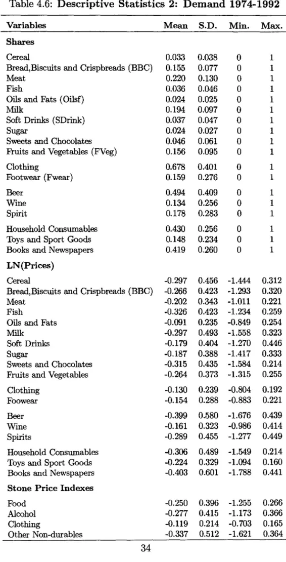
The data used on the demand side come from the UK Family Expenditure Surveys (FES) from 1974 to 1992. This survey has been widely used by studies investigating the properties of household consumption, savings and earnings5 . It contains information on household expenditures on a detailed set of goods (recorded in a two-week diary) and also on household composition. From the original data set, households whose head is higher than 60, self-employed or living in Northern-Ireland were excluded to keep a more homogenous sample. A list of the variables used and some descriptive statistics are presented in Tables 4.6 and 4.7 in the appendix.

The goods modelled here are cereal, breadjbiscuits, meat, fish, oilsjfats, milk, soft drinks, sugar, sweetsjchocolates and fruitsjvegetables in the food group. In the alcohol

5See Attanasio and Browning (1995) and Blundell, Duncan and Meghir (1995), for example.

group the focus is on beer, wine and spirits. The goods modelied in the clothing group are general clothing and footwear. Finally, the other non-durables group comprises household consumables, booksjnewspapers and toysjsport goods. The goods were defined so as to match the industry definition given by the UK Standard Industry Classification (1980)6. When a higher leveI of aggregation in the product definition was needed than one provided in the F.E.S., expenditures on the disaggregated goods were added and the price computed as a weighted average of each good's price, with weights given by the F.E.S. (reflecting the importance of the good for a representative UK consumer). The principal excluded goods were durables, vehicles and housing, to avoid the difficulties involved in modelling the dynamics involved in the household decision to buy these goods.

Figure 4.1 in the appendix shows the behavior of the expenditures in each group as shares of total non-durables expenditures over time. It appears that expenditures in alcohol and other non-durables have increased substantially over the last 15 years, after a drop in the 74-77 period. It also seems that, as expected, the food share has decreased markedly over the 1980's, while clothing expenditure's share showed a great deal of fluctuation in the period.

1.4. Results

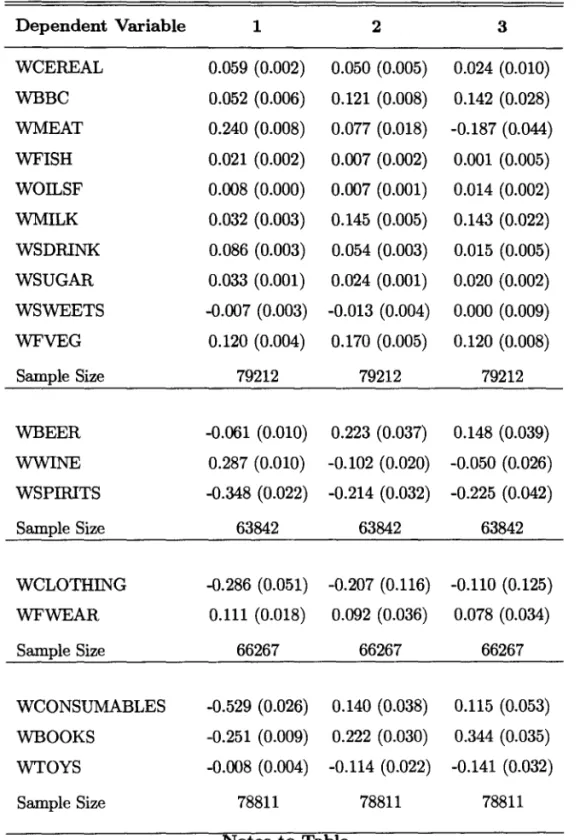
Table 1.1 reports estimated on the own-price coefficients in the individual share equa-tions. Each row shows the results of a particular share regression. The within-group Stone price index is used as a deflator throughout. In column (1) only own-price and (instrumented) total group expenditures are included. AlI own-price coefficients are significant and substantially different from each other, both within and between groups.

In column (2) the seasonal, demographic and compositional controls are also in-cluded. The price coefficients change significantly in most cases, confirming the impor-tance of including these controls in disaggregated regressions. These results would be the ones used to compute demand elasticities, had we restricted ourselves to analyzing only a particular good with these data. However, the results in column (3), where ali

Table 1.1: Own-Price Single-Equation Coefficient Estimates 1974-1992

Dependent Variable 1 2 3

WCEREAL 0.059 (0.002) 0.050 (0.005) 0.024 (0.010)

,

WBBC 0.052 (0.006) 0.121 (0.008) 0.142 (0.028)

WMEAT 0.240 (0.008) 0.077 (0.018) -0.187 (0.044)

WFISH 0.021 (0.002) 0.007 (0.002) 0.001 (0.005) WOILSF 0.008 (0.000) 0.007 (0.001) 0.014 (0.002) WMILK 0.032 (0.003) 0.145 (0.005) 0.143 (0.022) WSDRlNK 0.086 (0.003) 0.054 (0.003) 0.015 (0.005) WSUGAR 0.033 (0.001) 0.024 (0.001) 0.020 (0.002) WSWEETS -0.007 (0.003) -0.013 (0.004) 0.000 (0.009) WFVEG 0.120 (0.004) 0.170 (0.005) 0.120 (0.008)

Sample Size 79212 79212 79212

WBEER -0.061 (0.010) 0.223 (0.037) 0.148 (0.039) WWlNE 0.287 (0.010) -0.102 (0.020) -0.050 (0.026) WSPIRlTS -0.348 (0.022) -0.214 (0.032) -0.225 (0.042)

Sample Size 63842 63842 63842

WCLOTHING -0.286 (0.051) -0.207 (0.116) -0.110 (0.125) WFWEAR 0.111 (0.018) 0.092 (0.036) 0.078 (0.034)

Sample Size 66267 66267 66267

WCONSUMABLES -0.529 (0.026) 0.140 (0.038) 0.115 (0.053) WBOOKS -0.251 (0.009) 0.222 (0.030) 0.344 (0.035) WTOYS -0.008 (0.004) -0.114 (0.022) -0.141 (0.032)

Sample Size 78811 78811 78811

Notes to Table

Standard Errors in Parentheses. l. V. Estimates: instruments for ln(expenditure) are ln(income),

... change in real interest mtes and lagged unemployment mte. Contrals in column (1) are

ln(expenditure) and a constant termo Controls in column (2) are ln(expenditure), 3 seasonal, 10

regional, 15 demogmphic and

4

occupational variables and a time trend. Controls in column (3) are

"

those in column (2) plus all other group prices. The Stone price index for each group is used as defiator for the group prices throughout.

•

the other group prices are included, show that for goods like meat, fish, soft drinks, fruitjvegetables, beer, clothing and books, significant changes in the estimated own-price coeflicients can be observed. This emphasizes the risks associated with working only with individual goods. For other goods (breadjbiscuits, milk, sugar, spirits and footwear, for example) the inclusion of other prices does not dramatically change the own-price coeflicient.

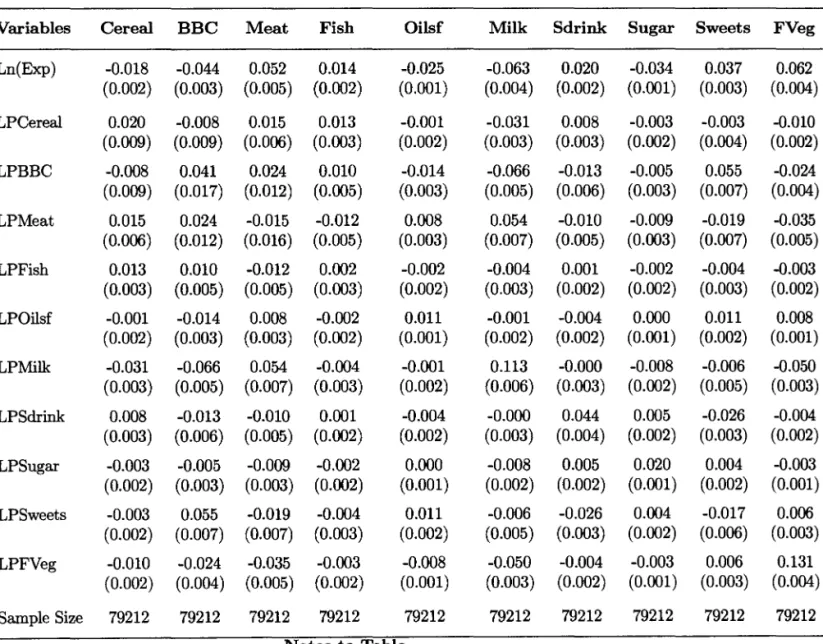
Tables 4.1 to 4.4 in the appendix report the results of estimating the symmetric constrained Almost Ideal Demand System for each group of non-durable goods7 • In the food system, the parameters are generally well-determined. Most own-price coeflicients are precisely estimated, the exceptions being meat and fish. With the estimated parameters predicted shares were computed for each good for each sample year, at the yearly average expenditures, prices and household characteristics. These shares (ú)i)

wiIl be used to compute the time-varying demand elasticities, according to equation (1.5).

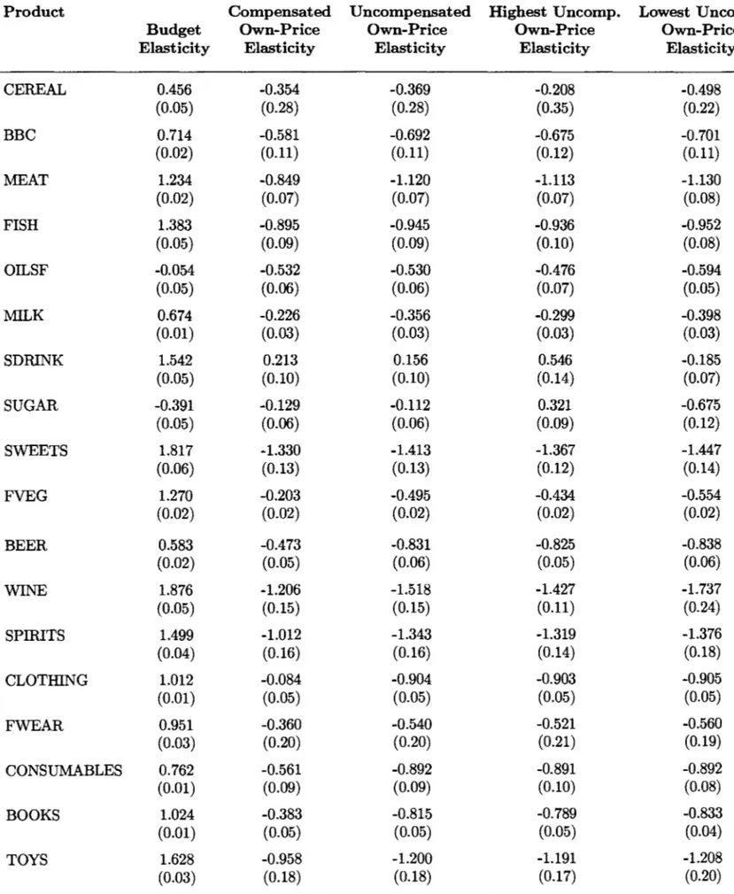
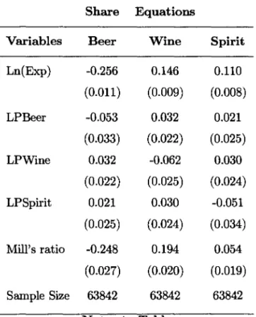
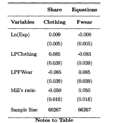
Table 4.2 presents the parameter estimates of the Alcohol system. The expenditure coeflicients are alI precisely estimated and so are the Mill's ratios ones, which confirms the importance of controlling for selectivity. The own-price coeflicient is precisely estimated in the wine equation and significant at 10% leveI in the beer and spirit equation. In Table 4.3 the results of estimating the clothing system are set out. Again, all the coeflicients in the Table are precisely estimated, although the expenditure ones only marginaIly so. Finally, Table 4.4 shows the parameter estimates of the other-non-durable goods. It reveals that while the expenditure and MiIl's ratio coeflicients are significant, the only significant own-price coeflicient appears in the book equation. This may occur either because the coeflicient is genuinely approximate zero both in the consumables and in the toys equations or because the estimate is not precise enough. In Table 1.2 the price and budget elasticities are set out. The results in the first column generally reveal an interesting and intuitive pattern. According to them, within the food system, meat, fish, soft drinks, sweetsjchocolates and fruitsjvegetables are luxuries while cereal, bread, milk are necessities and oilsjfats and sugar are inferior goods. In the alcohol system, beer is a necessity, while wine and spirits are luxuries.

Table 1.2: Price and Budget Elasticities 1974-1992

Product Compensated Uncompensated Highest U ncomp. Lowest U ncomp.

Budget Own-Price Own-Price Own-Price Own-Price

Elasticity Elasticity Elasticity Elasticity Elasticity

,

_{CEREAL 0.456} -0.354 -0.369 -0.208 -0.498

(0.05) (0.28) (0.28) (0.35) (0.22)

BBC 0.714 -0.581 -0.692 -0.675 -0.701

(0.02) (0.11) (0.11) (0.12) (0.11)

MEAT 1.234 -0.849 -1.120 -1.113 -1.130

(0.02) (0.07) (0.07) (0.07) (0.08)

FISH 1.383 -0.895 -0.945 -0.936 -0.952

(0.05) (0.09) (0.09) (0.10) (0.08)

OILSF -0.054 -0.532 -0.530 -0.476 -0.594

(0.05) (0.06) (0.06) (0.07) (0.05)

MILK 0.674 -0.226 -0.356 -0.299 -0.398

(0.01) (0.03) (0.03) (0.03) (0.03)

SDRlNK 1.542 0.213 0.156 0.546 -0.185

(0.05) (0.10) (0.10) (0.14) (0.07)

SUGAR -0.391 -0.129 -0.112 0.321 -0.675

(0.05) (0.06) (0.06) (0.09) (0.12)

SWEETS 1.817 -1.330 -1.413 -1.367 -1.447

(0.06) (0.13) (0.13) (0.12) (0.14)

FVEG 1.270 -0.203 -0.495 -0.434 -0.554

(0.02) (0.02) (0.02) (0.02) (0.02)

BEER 0.583 -0.473 -0.831 -0.825 -0.838

(0.02) (0.05) (0.06) (0.05) (0.06)

WINE 1.876 -1.206 -1.518 -1.427 -1.737

(0.05) (0.15) (0.15) (0.11) (0.24)

SPIRITS 1.499 -1.012 -1.343 -1.319 -1.376

(0.04) (0.16) (0.16) (0.14) (0.18)

CLOTHING 1.012 -0.084 -0.904 -0.903 -0.905

(0.01) (0.05) (0.05) (0.05) (0.05)

FWEAR 0.951 -0.360 -0.540 -0.521 -0.560

(0.03) (0.20) (0.20) (0.21) (0.19)

CONSUMABLES 0.762 -0.561 -0.892 -0.891 -0.892

(0.01) (0.09) (0.09) (0.10) (0.08)

BOOKS 1.024 -0.383 -0.815 -0.789 -0.833

ｾ＠ (0.01) (0.05) (0.05) (0.05) (0.04)

TOYS 1.628 -0.958 -1.200 -1.191 -1.208

(0.03) (0.18) (0.18) (0.17) (0.20)

Notes to Table

Elasticities Computed from Symmetric Consbhined Almost Ideal Model (Tables

_.

_.

4.1

to 4·4)·

•

There is no elear pattern in the elothing system, while there is some suggestion that household consumables are necessities and toysjsport goods are luxuries in the other non-durables one.

It can be seen in the second column that alI compensated own-price elasticities are negative, as the theory predicts, with the exception of the soft drinks one, which is only marginally different from zero. The average uncompensated price elasticities are set out in column (3). They show that in the food system, only meat and sweets are price elastic, though fish has an elasticity elose to one. Most of the elasticities are negative and significantly different from zero, with the exception of the soft drink one which is positive but insignificant and the cereal one which is insignificant. The alcohol goods alI have negative and significant elasticities with beer having an inelastic demando In the elothing system, elothing seems to be more elastic than footwear and in the other-goods one, toysjsport goods are the more elastic of the group.

The last two columns of the Table present the extreme values of the uncompensated price-elasticities over time. It can be seen that while the elasticity of goods like cereal, oilsjfats, milk, soft drink and sugar show a great deal of variation over time, others like beer, elothing, footwear and consumables show little variation. Figures 4.2 to 4.7 show graphically these patterns of variation, by plotting the values of the elasticities for each good over the sample period.

2. Matching

Supply

and Demand

2.1. The Matching Process

As seen above, the goods in the demand sector were defined in such a way as to facilitate the matching between industries and product definitions. In Table 2.1 the matching process is set out.

•

Table 2.1: Matching the

s.I.e.

with the Product Definitions

S.I.C. Code S.LC. Name Product Name.

411 Organic Oils and Fats Oils and Fats

412 Slaughtering of Animals and Production Beef+ lamb+ Pork+ Bacon+

of Meat and By-Products Poultry + Other meat

413 Preparation of Milk and Milk Products Milk + Milk Products

414 Processing of Fruits and Vegetables Fruit + Vegetables

415 Fish processing Fish

416 Grain Milling Cereals

419 Bread, Biscuits and Flour Confectionary Bread+Biscuits and cakes

420 Sugar and Sugar By-products Sugar

421 Ice Cream, Cocoa, Chocolate and Sugar

Confectionary Sweets and Chocolates

426 Soft Drinks Soft drinks

424 Spirit Distilling and Compounding Spirits

427 Brewing and Malting Beer

426 Wines, Cider and Perry Wines

436 Hosiery and Other Knitted Goods Men's outerwear+Women's Outerwear

+Children's outerwear+Other Clothing

451 Footwear Footwear

453 Clothing Men's outerwear+Women's Outerwear

+ Children's outerwear+Other Clothing

258 Soap and Toilet Preparations Household Consumables

475 Printing and Publishing Books and Newspapers

494 Toys and Sport Goods Toys, Photos and Sport Goods

•

these figures shows that in most cases the prices move quite dose together, which indicates that the matching process is satisfactory, especially if one takes into account the fact that other possible determinants of the behavior of retail prices, like the prices imported products and retailers' mark-ups, are not being controlled for.

In the data set used here, around 25% of firms operate in more than one three-digit S.Le. industry. Therefore, all industry leveI variables, induding the price elasticities, were matched to the firms in the sample using the information about the distribution of firms' sales across industries. For example, the price elasticity for a multi-product firm is the weighted average of the elasticity in each industry that the firm operates, with weights given by the ratio of the firm's sales in each industry to total firm's sales.

2.2. Identification

The usual problem with a procedure that tries to combine supply and demand data to investigate the interaction between consumers and firms is that market prices are joint1y determined by supply and demand behavior. Describe the profitability formula

by9;

(2.1) where

1]. = _(8q ) .Pjt

J 8p J qjt (2.2)

is the demand elasticity and Xit is a vector of variables refl.ecting market structure.

Shocks affecting firms' prices tend to affect both firms' profitability (direct1y) and the product market elasticity (through the retail price index), although the direction of the bias is not dear a priori. Positive product price shocks tend to increase the mark-up (2.1), but will increase the absolute value of 1]it only if the product demand is

inelastic, decreasing it otherwise. Given that 13 out of the 18 products in Table (1.2) have inelastic demands on average (column 3) and that one would expect a negative relationship between profitability and the absolute value of the elasticity, one can tentatively predict that the ordinary least squares estimate of 'Y would be downwards

biased (in absolute value)lO.

This bias can be reduced by examining the joint response of both the mark-ups and the elasticities to variables that affect demand and are orthogonal to the supply shocks. As shown in Shea (1993, 1996), the usefulness of the instrument set depends on its exogeneity (absence of correlation between instrument set and supply shocks) and relevance (presence of correlation between instrument set and demand elasticities). Recent research has shown that low relevance can increase the inconsistency of I. V. estimates whenever the instruments are not perfectly exogenous and can even affect the consistency of perfectly exogenous instruments in small samples11 .

One of the advantages of the procedure used in this paper is that household char-acteristics, available from the survey data, provide a unique way of identifying the supply equation. The fitted values of the Almost Ideal Equation estimated in the last section are:

Wjt =

&j

+

L:1Jk

1og(Pkt)

+

ｾｬｯｧＨｾｴＩ＠

k t

(2.3)

&j

=

ao

+

L:

&j

Zit

+

8T

+

Js

(2.4)

so that the price elasticities were computed according to:

1;;

-'f/jt = --;:::- -

/3j -

1

Wjt (2.5)

where Wjt are the predicted shares. Thehousehold characteristics variables Zit

en-ter the share equations in order to reflect differences in household preferences and composition, that affect shares and may be correlated with total expenditures and prices.

First-differencing (2.5) one gets:

(2.6)

so that, as

1;;

does not vary over time, the time variation of the elasticities is deter-mined by the variation in the predicted Wjt 's. The time-varying household charac-teristics Zkt will, by construction, affect the predict shares and hence the elasticities,

lOQne could then ask why don't the producers increase prices in the face of an inelastic product

ｾ＠ demando But of course the elasticity facing an individual producer also depends on the behaviour of its competitors.

llSee Staiger and Stock (1994), Nelson and Startz (1990) and Bound, Jaeger and Baker (1995).

thereby fulfilling (in theory) the relevance criteria. These are age, age squared, number of adults, number of adults squared, number of females, a single parent dummy, num-ber of kids in various age groups and five occupational dummies12 • Moreover, there is no reason to expect these variables to affect the firms' pricing behavior, conditional on their effect on the demand elasticities. In order to construct the instrument set, yearly weighted averages of the household characteristics were computed for each product, using each household's expenditure on the product as a percentage of total product expenditure in a given year as weights. AlI variables will be used in first-differences.

In order to check whether the relevance criterion is also fulfilled in practice13 , the tables below report partial

R2

and F statistics on the excluded instruments in a first-stage regression of the demand elasticities on the instrument set. Since the equations estimated contain more than one endogenous variables, the partial R2 _{statistics are}

computed according to Shea (1996), who describes a method to measure the relevance of the instrument set for each endogenous variable, even if the instruments are highly collinear. The essence of the procedure is to compute the squared correlation be-tween the values of the endogenous variable of interest, orthogonalized with relation to the other endogenous variables, and the fitted values of it (from a regression on the instrument set), again orthogonalized with relation to the fitted values of the other endogenous variables.

As another check of the validity of instruments, the results of this procedure will be compared with a more traditional Generalized Method of Moments procedure, that uses lagged values of the endogenous variables as instruments14 • This procedure has often been criticized on the basis of the relevance criteria, since the persistence of the majority of micro variables over time could mean that lagged values of them are only weakly correlated with their first-difference values15 . The validity of this procedure also hinges on the absence of serial correlation in the leveIs specification.

In order to complete the identification procedure and examine the effect of

con-12The household characteristics are summarized in Table 4.7.

13In practice, the relevance depends on the importance of the household composition variables in each share equation. The full estimated equations are available from the author upon request.

14See Arellano and Bond (1991).

sumer behavior on firms' mark-ups, it is necessary to discuss the consistency of the estimates of the price parameter in the share equation

fjj.

In this case, as prices have only time series variation, the use of micro data alleviates the problem of simultane-ity, as long as there are no common aggregate shocks in the error term (see Goldberg, 1995). The inclusion of seasonals, total expenditures and a time trend in the share equations helps removing these aggregate terms out of the errors.

2.3. Data

On the supply side, this paper uses data on company accounts available from the U.K. Datastream on-line service. The industry leveI information comes from the U.K. Census of Production. The criteria for selecting firms was that they operated in the consumer non-durables sector of the economy and that information was available both on the distribution of sales across different industries and on the percentage of sales that is sold abroad. We were left with an unbalanced sample of 161 firms operating from 1974 to 1992.

The dependent variable used throughout this study is accounting pre-tax profits (before depreciation allowances) divided by total sales16_{• The other firm leveI variables}

are market share and capital/sales. The market share variable traditionally used in S.C.P. studies is the ratio of firm's total sales to its main industry sales. However, many fums are diversified and operate across different industries. Therefore, the first step towards improving the market share variable is to use the sales distribution information to compute a market share for each industry in which the firm operates and calculate the weighted average of these market shares, with the weights being the percentage of the firm's sales in each industry17. The second step is to use only the

firm's domestic sales in the numerator and exclude industry exports from the total industry sales in the denominator, in order to concentrate on the relationship between the firm's domestic market share and its profitability.

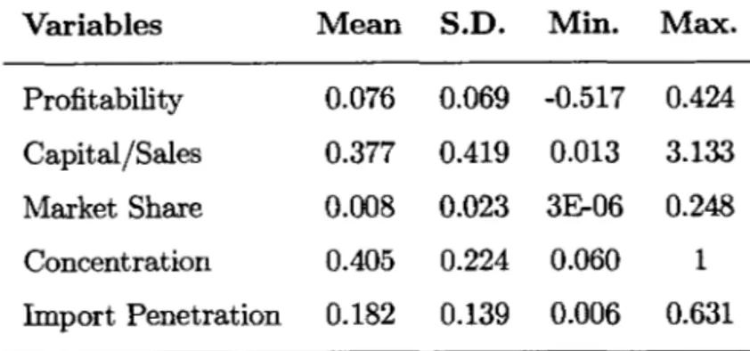
Finally, the industry leveI variables used in this study are the five-firm concentra-tion ratio and import penetraconcentra-tion (imports/sales). Table 4.5 in the appendix presents

16For a comparison between this measure and Tobin's q see Stevens (1990).

17UnforttUlately, with the data I use the information on sales' distribution begins only in 1979 for some firms and in 1980 for the others. Therefore, we used the 1979/80 weights from 1975-79.

some descriptive statistics of the firm and industry leveI variables used in this paper. 2.4. Results

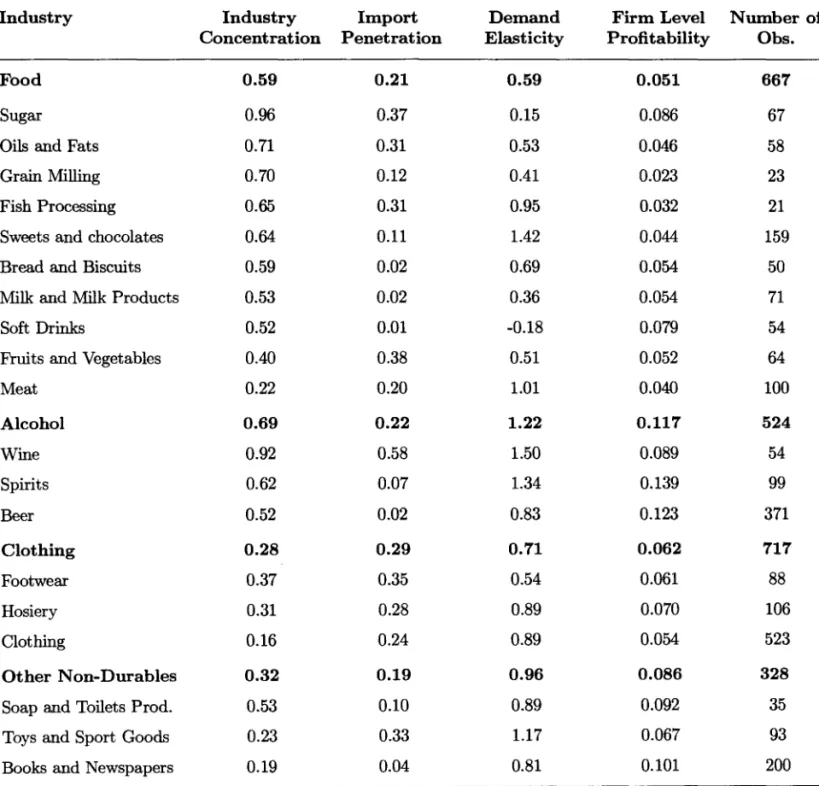
In this section, the estimated time-varying uncompensated demand elasticities wilI be used as independent variables in profitability regressions, in order to examine the effect that consumer behavior may have on the firms' mark-ups. Table (2.2) describes the variation in the demand elasticity variable across industries and its relationship with the average concentration ratio, import penetration and firm leveI profitability over the sample period. The industries are listed in decreasing order of concentration ratio within each group.

The table shows that industries with the lowest elasticity in the food group, like sugar and soft drinks, have the highest average profitability, although with very differ-ent concdiffer-entration and import penetration ratios from each other. The reverse occurs with products like sweetsjchocolates and meat, the only ones with elastic demands in the group, both with lower than average profitability despite very different leveIs of concentration and import penetration. A similar story is to be found in the alco-hol group, specially in a comparison between the wine and beer industries, although import penetration may have an important role in this case. In the clothing group, alI industries tend to have low concentration, inelastic demands and low profitability. Finally, in the other non-durables group, booksjnewspapers have a much lower con-centration ratio than the soapsjtoilet products industry, but both have above average profitability, in line with their relatively inelastic demando

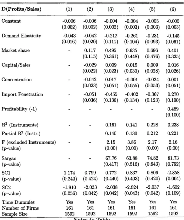
Table 2.3 shows the results of estimating the demand elasticities' impact on prof-itability. AlI models in this table are estimated in differenced form, in order to capture the relationship between changes in profitability and changes in elasticity, which could not be captured through the inclusion of industry dummies.

Table 2.2: Data Description: 1975-1992

Sample Means

Industry Industry Import Demand Firm LeveI Number of

Concentration Penetration Elasticity Profitability Obs.

Food 0.59 0.21 0.59 0.051 667

Sugar 0.96 0.37 0.15 0.086 67

Oils and Fats 0.71 0.31 0.53 0.046 58

Grain Milling 0.70 0.12 0.41 0.023 23

Fish Processing 0.65 0.31 0.95 0.032 21

Sweets and chocolates 0.64 0.11 1.42 0.044 159

Bread and Biscuits 0.59 0.02 0.69 0.054 50

Milk and Milk Products 0.53 0.02 0.36 0.054 71

Soft Drinks 0.52 0.01 -0.18 0.079 54

Fruits and Vegetables 0.40 0.38 0.51 0.052 64

Meat 0.22 0.20 1.01 0.040 100

A1cohol 0.69 0.22 1.22 0.117 524

Wine 0.92 0.58 1.50 0.089 54

Spirits 0.62 0.07 1.34 0.139 99

Beer 0.52 0.02 0.83 0.123 371

Clothing 0.28 0.29 0.71 0.062 717

Footwear 0.37 0.35 0.54 0.061 88

Hosiery 0.31 0.28 0.89 0.070 106

Clothing 0.16 0.24 0.89 0.054 523

Other Non-Durables 0.32 0.19 0.96 0.086 328

Soap and Toilets Prod. 0.53 0.10 0.89 0.092 35

Toys and Sport Goods 0.23 0.33 1.17 0.067 93

Books and Newspapers 0.19 0.04 0.81 0.101 200

Table 2.3: Demand Elasticity and Profitability: 1979-1992

D(ProfitsjSales) (1) (2) (3) (4) (5) (6)

Constant -0.006 -0.006 -0.004 -0.004 -0.005 -0.005

(0.002) (0.002) (0.002) (0.003) (0.003) (0.003) Demand Elasticity -0.043 -0.042 -0.212 -0.261 -0.231 -0.145 (0.016) (0.020) (0.111) (0.104) (0.093) (0.061)

Market share 0.117 0.495 0.635 0.696 0.401

(0.115) (0.361) (0.448) (0.476) (0.325)

Capital jSales -0.029 0.009 0.015 0.009 0.016

(0.022) (0.023) (0.030) (0.028) (0.026)

Concentration -0.042 0.017 -0.001 -0.024 0.001

(0.023) (0.051) (0.055) (0.053) (0.051)

Import Penetration -0.051 -0.455 -0.402 -0.367 0.270

(0.036) (0.136) (0.134) (0.123) (0.100)

Profitability (-1) 0.489

(0.100)

R2 (Instnunents) 0.161 0.141 0.228 0.238

Partial R2 (Instr.) 0.140 0.130 0.212 0.221

F (excluded Instruments) 2.15 3.86 2.17 2.16

(p-value) (0.00) (0.00) (0.00) (0.00)

Sargan 67.76 63.88 74.82 81.73

(p-value) (0.417) (0.516) (0.643) (0.792)

SCl 1.174 0.799 0.772 0.837 0.806 -2.858

(p-value) (0.240) (0.424) (0.440) (0.403) (0.420) (0.004)

SC2 -1.910 -2.033 -2.038 -2.024 -2.037 -1.602

(p-value) (0.056) (0.042) (0.042) (0.043) (0.042) (0.109)

Time Dummies Yes Yes Yes Yes Yes Yes

Number of Firms 161 161 161 161 161 161

Sample Size 1592 1592 1592 1592 1592 1592

Notes to Table

Standard Errors in Parentheses. All Models estimated in First-DijJerences. OLS estimates in

columns 1 and 2. 1. V. estimates in columns 3 to 6. Instruments used in column 3: household

composition variables plus lagged values (t-3) of RHS variables except for elasticity. Instruments

used in column

4:

lagged values (t-3) of all RHS variables. Instruments used in column 5: those in

column 3 plus those in column

4.

Instruments used in column 6: those in column 5 plus lagged

absolute value of the estimated demand elasticity coeffi.cient is about five times higher than the one in column (2). The other right-hand-side variables are instrumented with their own values lagged three periods. The

R2

and the partial-R2 _{on the excluded}

in-struments are 0.16 and 0.14 respectively, showing that, although a small part of the explanatory power of the instrument set is not relevant for the elasticity variable, it still explains a significant part of the elasticities' variation over time. The F-statistic on the joint significance of the household characteristics in the elasticity equation con-firms the relevance of the instruments. If these characteristics are not included in the instrument set, the elasticity coeffi.cient drops (in absolute value) back to -0.034

(0.036).

In column (4), lagged values of the elasticity variable are included instead ofthe household variables. Perhaps surprisingly, the elasticity coeffi.cient also shows up very strongly and precisely estimated. The

R2

and the partial-

R2

on the excluded instru-ments are 0.14 and 0.13 respectively (lower than in column (3)) and the F-statistic also rejects the null of instrument irrelevance. The similarity between the results of columns (3) and (4) is very reassuring and points to the inclusion of both set of in-struments in the same specification, which is done in column (5). As expected, the standard error in this specification is lower than in the previous columns and the estimated coeffi.cient does not change much. Finally, column (6) includes a lagged de-pendent variable as a robustness test that confirms the results obtained thus faro The results in this column suggest that, at the mean profitability and elasticity values in the sample, an increase of one standard deviation in the absolute value of the elasticity would decrease profitability by around 121% in the long run, a very tangible effect18_• With respect to the other determinants of profitability, the results of column (5) are somewhat mixed. The market share coeffi.cient is very high but only significant at the 15% level. The import penetration variable enters strongly and significantly, while the concentration coeffi.cient is insignificantly different from zero. As it is well known, economists have long debated whether the impact of market structure variables on

18The long run proportional effect is ＨＱｾｏｏｾＺＺＹＩ＠ ｧＺｾＪｾ＠ = -3.22. Therefore, an increase of one stan-dard deviation in the deIDand elasticity (0.346 in the sample, or 37% of the IDean) would decrease profitability by about 121%.

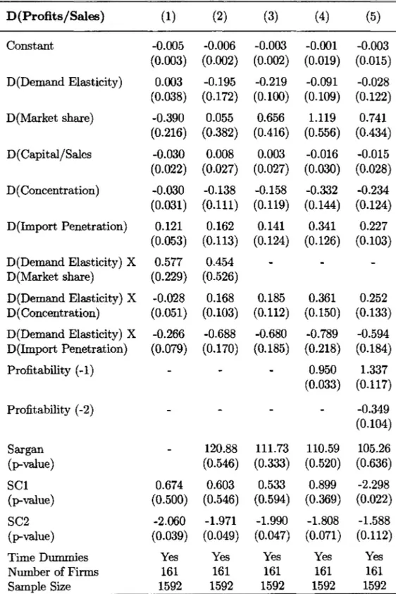
Table 2.4: Demand Elasticity and Structural Variables

D(Profits /Sales) (1) (2) (3) (4) (5)

Constant -0.005 -0.006 -0.003 -0.001 -0.003

(0.003) (0.002) (0.002) (0.019) (0.015) D(Demand Elasticity) 0.003 -0.195 -0.219 -0.091 -0.028 (0.038) (0.172) (0.100) (0.109) (0.122)

D(Market share) -0.390 0.055 0.656 1.119 0.741

(0.216) (0.382) (0.416) (0.556) (0.434) D( Capital/Sales -0.030 0.008 0.003 -0.016 -0.015 (0.022) (0.027) (0.027) (0.030) (0.028) D( Concentration) -0.030 -0.138 -0.158 -0.332 -0.234 (0.031) (0.111) (0.119) (0.144) (0.124) D(Import Penetration) 0.121 0.162 0.141 0.341 0.227

(0.053) (0.113) (0.124) (0.126) (0.103) D(Demand Elasticity) X 0.577 0.454

D(Market share) (0.229) (0.526)

D(Demand Elasticity) X -0.028 0.168 0.185 0.361 0.252 D( Concentration) (0.051) (0.103) (0.112) (0.150) (0.133) D(Demand Elasticity) X -0.266 -0.688 -0.680 -0.789 -0.594 D(Import Penetration) (0.079) (0.170) (0.185) (0.218) (0.184)

Profitability (-1) 0.950 1.337

(0.033) (0.117)

Profitability (-2) -0.349

(0.104)

Sargan 120.88 111.73 110.59 105.26

(p-value) (0.546) (0.333) (0.520) (0.636)

SC1 0.674 0.603 0.533 0.899 -2.298

(p-value) (0.500) (0.546) (0.594) (0.369) (0.022)

SC2 -2.060 -1.971 -1.990 -1.808 -1.588

(p-value) (0.039) (0.049) (0.047) (0.071) (0.112)

Time Dummies Yes Yes Yes Yes Yes

Number of Firms 161 161 161 161 161

Sample Size 1592 1592 1592 1592 1592

Notes to Table

.

_{Standard Errors in Parentheses. OLS Estimates in column 1. 1. V. Estimates in columns 2 to 5.}

Instruments used: Household Characteristics + Lagged values (t-3) of all included variables.

First-Differences Specification in columns 1, 2 and 3. Quasi-Differences Specification in columns 4

profitability reflects 'tacit collusion' or 'differential efficiency'19. The fact that demand elasticities have been estimated can perhaps shed some more light on this issue from a different point of view.

Even the most collusive group of firms will be impotent to increase prices and profits if facing a very elastic demand pattern20 . Therefore, if industry concentra-tion facilitated collusion (that translated into higher profits) and import penetraconcentra-tion hindered it, then the positive concentration and the negative import effects on prof-itability would be stronger in industries where product demand was more inelastic. If, on the other hand, both effects were found to be stronger in industries where the potential for consumer exploitation is low, then the collusion hypothesis would not be very attractive and some variant of the 'differential efficiency' argument would be more compelling.

Column (1) in Table (2.4) reports the results of ordinary least squares estimation of a specification that interacts the demand elasticity with the market structure vari-ables. There is some evidence that both the market share effect and the negative import effect are stronger in more elastic industries. The results of column (2), where household characteristics and lagged values of the right-hand-side variables are used as instruments, show that both the concentration and the import penetration effects are much stronger in the more elastic industries which does not lend support to the 'collusion' hypothesis. It seems however, that the market share result is not robust to endogeneity so that, in column (3), the market share interaction is dropped with no effect in the main results.

In columns (4) and (5), the results of a quasi-differences specification are set out. This specification, first suggested by Holtz-Eakin et al (1988) is more general than the first-differences one, as it allows for a time-varying fixed effect coefficient and includes the leveI of the right-hand-side variables in the regressions as well:

(2.7)

19See Shepherd (1986), Smirlock, Gilligan and Marshall (1986) and Stevens (1990).

20The limiting case is the monopoly model, where the mark-up equals the inverse of the price elasticity.

where ao is a constant, ai is the firm specific effect, "( and {3 are parameters to be estimated and cit is a random error termo By lagging (2.7) one period, solving for ai

and substituting back in (2.7) one gets a quasi-differences specification:

Yit = (1 - "()ao

+

{3Xit - ({3"()Xit- 1

+

"(Yit-l

+

cit - "(Cit-l (2.8) This expression can be estimated by applying an I.V. approach to:

(2.9)

Where a = (1 - "()ao, b1 = {3, b2 = ({3 - (3"(), c = "( and Vt = cit - ("()Cit-l.

In column (4), the results of the quasi-differences specification are set out. A test

for the first-differences specification, in which c

=

1 and alI components of b2

=

O,

resulted in X2 (8)

=

15.70 with p

=

0.047, marginally rejecting the first-differences

specification. Moreover, the observed increase in most of the estimated coefficients shows that this specification does indeed make a difference. The estimated value for

"( (= 0.950) means that the effect of firm specific components on profitability tend to decrease over time. The qualitative results, however, do not change. In the last

column, another lag of the dependent variable is included as a robustness test, which does not change the main results either. This can be seen as evidence that the impact of concentration on the firms' mark-ups in this period does not seem to be related to collusive practices and that the import penetration effect decreased profitability through its effect on the prices of more competitive industries.

3. Conclusions

This paper used two independent data sets, one with firm and industry leveI data and the other with information on household characteristics and expenditures, to integrate demand side issues into empirical Structure-Conduct-Performance models.

In a recent review of their own work, Connor and Peterson (1997) state that "of all

incorporate cross-price or demographic effects other than income; standard theoretical demand restrictions were neither imposed nor examined; possible price endogeneity was not controlled for; the level of aggregation was greater than that of our price data; the time period used is now quite dated; and many of the elasticity estimates were suspiciously low in absolute value" (p. 225). Each of these points was addressed in this paper.

The very detailed product definitions in the UK Family Expenditure Surveys al-lowed the products in the demand side to be defined so as to match the

s.l.e.

defini-tions traditionally used in supply side studies. Moreover, the household characteristics, also available from the household surveys, were used to construct a unique instrument set, uncorrelated with the firms' supply decisions. The parameters of Almost Ideal Demand Systems for four groups of goods (food, alcohol, clothing and other non-durables) were estimated using time series of cross-sectional household data. The resulting budget and price elasticities accorded to demand theory and showed quite interesting and intuitive patterns. In particular, time-varying uncompensated price elasticities were computed that showed substantial cross-section and time-series vari-ation. The estimated price elasticities were matched to several consumer industries where the firms in our sample operate and then included in profitability equations to examine the impact of consumer demand on firms' performance.

The results indicated that demand elasticities have a significant and sizable neg-ative effect on profitability and that controlling for their endogeneity substantially increases the absolute value of the estimated coefficients. Similar results were oh-tained when household characteristics and lagged values of the elasticities were used alternatively as instruments in the estimated equations. Finally, in our sample pe-riod industry concentration and import penetration had a more pronounced impact on profitability in more competitive environments that is, where demand was more elastic, a finding that does not fit in very well with the 'collusion' explanation for the impact of market structure variables on firms' performance.

The integration of demand side issues into the standard supply side framework raises several new questions that were never considered in the literature and that this study has only started investigating. In this paper, for example, the slope of

the demand curve was assumed constant throughout the sample period, but there are reasons why one might want to relax this assumption and allow the slope to vary over the business cycle, for example. Future work in this area might want to focus on the determinants of the behavior of demand elasticities over the business cycle and their relationship with the cyclicality of mark-ups (see Bils, 1989, Chevalier and Scharfstein, 1996 and Rotemberg and Woodford, 1991). Another potentially interesting idea would be to examine the relationship between income distribution and corporate performance. The price elasticity of the demand for a product, for example, can be decomposed into different elasticities for different levels of the expenditure distribution (see Blundell et aI, 1993). Moreover, there is some evidence that the expenditure distribution is correlated with the earnings distribution (see Attanasio and Davies, 1997). It would perhaps be interesting to examine whether the recent rise in the wage dispersion in the UK and US, for example, have afIected the behavior of firms through its impact on expenditures and demando

References

[1] Arellano. M. and Bond, S. (1991). 'Some Tests of Specification for Panel Data: Monte Carlo Evidence and an application to Employment Equations'. Review of

Economic Studies, voI. 58, pp. 277-297.

[2] Attanasio, O. and Browning, M. (1995). 'Consumption over the Life Cycle and over the Business Cycle'. American Economic Review, voI. 85, no. 5, pp. 1118-37. [3] Attanasio, O. and Davies, S. (1996). Relative Wage Movements and the

Dis-tribution of Consumption'. Journal of Political Economy, voI. 104, no. 6, pp. 1227-1262.

[4] Banks, J. , Blundell, R. and Lewbel, A. (1994). 'Quadratic Engel Curves, lndirect Tax Reform and Welfare Measurement'. University College London Discussion Paper, no. 94-04.

[6] Bils, M. (1989). 'Pricing in a Customer Market'. Quarterly Journal of Economics,

voI. 104, no. 4, pp. 699-718.

[7] Blundell,

R,

Duncan, A. and Meghir, C. (1995). ' Estimating Labor Supply Responses using Tax Reforms'. Institute for Fiscal Studies Working Paper, no. W95/7.

[8] Blundell,

R,

Pashardes, P. and Weber,G. (1993). 'What Do We Learn About Consumer Demand Patterns from Micro Data ?'. American Economic Review,

voI. 83, no. 3, pp. 570-597.

[9] Bound, M., Jaeger, D. and Baker,

R

(1995). 'Problems with Instrumental Vari-ables Estimation when the correlation between the Instruments and the Endoge-nous Explanatory Variable is Weak'. Journal of the American Statistical Associ-ation, voI. 90, pp. 443-450.

[10] Browning, M. and Meghir,C. (1991). 'The Effects of Male and Female Labor Supply on Commodity Demands'. Econometrica, voI. 59, no. 4, pp. 925.51.

[11]

Chevalier, J. and Scharfstein, D. (1996). 'Capital Market Imperfections and

Coun-tercyclical markups: Theory and Evidence'. American Economic Review, voI. 86, no. 4, pp. 703-725.

[12] Comanor, W. and Wilson, T. (1974). Advertising and Market Power. Cambridge: Harvard University press.

[13] Connor, J. and Peterson, E. (1992). 'Market-Structure Determinants of National Brand-Private Label Price Differences of Manufactured Food Products', The Journal of Industrial Economics, voI. 40, no. 2, pp. 157-170.

[14] Connor, J. and Peterson, E. (1997). "Market-Structure Determinants ofNational Brand-Private Label Price Differences of Manufactured Food Products: Reply',

The Journal of Industrial Economics, voI. 45, no. 2, pp. 225-226.

[15] Deaton, A. and Muellbauer, J. (1980). 'An Almost Ideal Demand System'. Amer-ican Economic Review, voI. 70, pp. 312-326.

27

[16] Goldberg, P. (1995). 'Product Differentiation and Oligopoly in International mar-kets: The Case of the USo Automobile Industry'. Econometrica, vol. 63, no. 4, pp. 891-951.

[17] Griliches, Z. and Mairesse, J. (1995). ' Production Functions: The Search for Identification'. Harvard University, mimeo.

[18] Hamermesh, D. (1993) Labor Demand. Priceton University Press. Princeton, N.J.

[19] Heckman, J. (1979). 'Sample Selection Bias as a Specification Error'. Economet-rica, vol. 47, pp. 153-61.

[20] Holtz-Eatkin, D. , Newey, W. and Rosen, H. (1988). 'Estimating Vector Autore-gressions with Panel Data'. Econometrica, vol. 56, pp.1371-95.

[21] Klette, T. (1996). 'R&D, Scope Economies, and Plant Performance'. Rand Jour-nal of Economics, vol. 27, no. 3, pp. 502-522.

[22] Layard, R., Nickell, S. and Jackman, R., (1991). Unemployment: Macroeconomíc Performance and the Labour Market. Oxford: Oxford University Press.

[23] Lewbel, A. (1996a). ' Aggregation Without Separability: a Generalized Compos-ite Commodity Theorem'. American Economic Review, vol. 86, no.3, pp. 524-543.

[24] Lewbel, A. (1996b). ' Large Demand Systems and Nonstationary Prices: Income and Price Elasticities for Many USo Goods '. Brandeis University, mímeo.

[25] Nelson, C. and Startz, R. (1990). 'The distribution of the Instrumental Vari-able Estimator and its T-Ratio when the Instrument is a Poor One'. Journalof

Busíness, vol. 58, pp. 125-140.

[26] Nevo, A. (1997). 'Measuring Market Power in the Ready-to-Eat Cereal Industry'. Harvard U niversity, mímeo.

[28] Rotemberg,

J.

and Woodford, G. (1991). 'Markups and the Business Cycle'.

Macroeconomics Annual, vol. 6, pp. 63-129.

[29] Rothenberg, T. (1973). Efficient Estimation with A Priori Information. Cowles Foundation Monograph 23. New Haven: Yale University Press.

[30] Schmalensee, R. (1989). 'Inter-Industry Studies of Structure and Performance'

in R. Schmalensee and R.D. Willig (eds). Handbook of Industrial Organization: Volume II: North-Holland, Amsterdam.

[31] Shea,

J.

(1996). 'Instrument Relevance in Multivariate Linear Models: a Simple Measure'. NBER Technical Working Paper, no.193.

[32] Shea,

J.

(1993). 'Do Supply Curves Slope Up?' Quarterly Journal of Economics,

vol. 108, no.l, pp.I-32.

[33] Shepherd, W. (1986). 'Tobin's q and the Structure-Performance Relationship: a Comment'. American Economic Review, voI. 76, pp. 1203-1209.

[34] Smirlock, M., Gilligan, T. and Marshall, W. (1986). 'Tobin's q and the Structure-Performance Relationship: a Reply'. American Economic Review, voI. 76, pp. 1211-1213.

[35] Staiger, D. and Stock,

J.

(1994). 'Asymptotics for Instrumental Variables Regres-sions with Weakly Correlated Instruments'. NBER Technical Working Paper, no. 161, forthcoming, Econometrica.

[36] Stevens,

J.

(1990). 'Tobins'q and the Structure-performance Relationship: A Com-ment'. American Economic Review, vol.80, no.3, pp.619-623.

[37] Working, E. (1927). 'What do Statistical Demand Curves Show?' Quarterly Jour-nal of Economics, voI. 41, pp. 212-235.

4. Appendix

4.1. Tables

Table 4.1: The Almost Ideal Demand System - Food

Share Equations

Variables Cereal BBC Meat Fish Oilsf Milk Sdrink Sugar Sweets FVeg

Ln(Exp) -0.018 -0.044 0.052 0.014 -0.025 -0.063 0.020 -0.034 0.037 0.062

(0.002) (0.003) (0.005) (0.002) (0.001) (0.004) (0.002) (0.001) (0.003) (0.004)

LPCereal 0.020 -0.008 0.015 0.013 -0.001 -0.031 0.008 -0.003 -0.003 -0.010

(0.009) (0.009) (0.006) (0.003) (0.002) (0.003) (0.003) (0.002) (0.004) (0.002)

LPBBC -0.008 0.041 0.024 0.010 -0.014 -0.066 -0.013 -0.005 0.055 -0.024

(0.009) (0.017) (0.012) (0.005) (0.003) (0.005) (0.006) (0.003) (0.007) (0.004)

LPMeat 0.015 0.024 -0.015 -0.012 0.008 0.054 -0.010 -0.009 -0.019 -0.035

(0.006) (0.012) (0.016) (0.005) (0.003) (0.007) (0.005) (0.003) (0.007) (0.005)

LPFish 0.013 0.010 -0.012 0.002 -0.002 -0.004 0.001 -0.002 -0.004 -0.003

(0.003) (0.005) (0.005) (0.003) (0.002) (0.003) (0.002) (0.002) (0.003) (0.002)

LPOilsf -0.001 -0.014 0.008 -0.002 0.011 -0.001 -0.004 0.000 0.011 0.008

(0.002) (0.003) (0.003) (0.002) (0.001) (0.002) (0.002) (0.001) (0.002) (0.001)

LPMilk -0.031 -0.066 0.054 -0.004 -0.001 0.113 -0.000 -0.008 -0.006 -0.050

(0.003) (0.005) (0.007) (0.003) (0.002) (0.006) (0.003) (0.002) (0.005) (0.003)

LPSdrink 0.008 -0.013 -0.010 0.001 -0.004 -0.000 0.044 0.005 -0.026 -0.004

(0.003) (0.006) (0.005) (0.002) (0.002) (0.003) (0.004) (0.002) (0.003) (0.002)

LPSugar -0.003 -0.005 -0.009 -0.002 0.000 -0.008 0.005 0.020 0.004 -0.003

(0.002) (0.003) (0.003) (0.002) (0.001) (0.002) (0.002) (0.001) (0.002) (0.001)

LPSweets -0.003 0.055 -0.019 -0.004 0.011 -0.006 -0.026 0.004 -0.017 0.006

(0.002) (0.007) (0.007) (0.003) (0.002) (0.005) (0.003) (0.002) (0.006) (0.003)

LPFVeg -0.010 -0.024 -0.035 -0.003 -0.008 -0.050 -0.004 -0.003 0.006 0.131

(0.002) (0.004) (0.005) (0.002) (0.001) (0.003) (0.002) (0.001) (0.003) (0.004)

Sample Size 79212 79212 79212 79212 79212 79212 79212 79212 79212 79212

Notes to Table

Table 4.2: The Almost Ideal Demand System - Alcohol

Share Equations

Variables Beer Wine Spirit

Ln(Exp) -0.256 0.146 0.110

(0.011) (0.009) (0.008)

LPBeer -0.053 0.032 0.021

(0.033) (0.022) (0.025)

LPWine 0.032 -0.062 0.030

(0.022) (0.025) (0.024)

LPSpirit 0.021 0.030 -0.051

(0.025) (0.024) (0.034)

Mill's ratio -0.248 0.194 0.054 (0.027) (0.020) (0.019)

Sample Size 63842 63842 63842

Notes to Table

Symmetric Constmined Estimates. Standard Errors in Parentheses. Instruments for ln(expenditure) in the first step are ln(income), change in real interest mtes and lagged unemployment mte.

Table 4.3: The Almost Ideal Demand System - Clothing

Share Equations

Variables Clothing Fwear

Ln(Exp) 0.009 -0.009

(0.005) (0.005)

LPClothing 0.085 -0.085

(0.039) (0.039)

LPFWear -0.085 0.085

(0.039) (0.039)

Mill's ratio -0.050 0.050 (0.016) (0.016)

Sample Size 66267 66267

Notes to Table

•

_.

Table 4.4: The Almost Ideal Demand System - Other Non-Durables

Share Equations

Variables Toys Books Consumables

Ln(Exp) 0.093 0.010 -0.103

(0.004) (0.005) (0.005)

LPToys -0.016 -0.032 0.048

(0.027) (0.015) (0.030)

LPBooks -0.032 0.082 -0.050

(0.015) (0.019) (0.019)

LPConsumables 0.048 -0.050 0.002

(0.030) (0.019) (0.039)

Mill's ratio 0.176 0.442 -0.618

(0.057) (0.071) (0.066)

Sample Size 78811 78811 78811

Notes to Table

Symmetric Constroined Estimates. Standard Errors in Parentheses. Instruments for ln(expenditure) in the first step are ln(total income), change in real interest rotes and lagged unemployment rote.

Table 4.5: Descriptive Statistics 1: Supply 1975-1992

Variables Mean S.D. Min. Max.

Profitability 0.076 0.069 -0.517 0.424

Capital/Sales 0.377 0.419 0.013 3.133

Market Share 0.008 0.023 3&06 0.248

Concentration 0.405 0.224 0.060 1

Import Penetration 0.182 0.139 0.006 0.631

Table 4.6: Descriptive Statistics 2: Demand 1974-1992

Variables Mean

s.n.

Min. Max.

Shares

Cereal 0.033 0.038 O 1

Bread,Biscuits and Crispbreads (BBC) 0.155 0.077 O 1

Meat 0.220 0.130 O 1

Fish 0.036 0.046 O 1

Oils and Fats (Oilsf) 0.024 0.025 O 1

Milk 0.194 0.097 O 1

Soft Drinks (SDrink) 0.037 0.047 O 1

Sugar 0.024 0.027 O 1

Sweets and Chocolates 0.046 0.061 O 1

Fruits and Vegetables (FVeg) 0.156 0.095 O 1

Clothing 0.678 0.401 O 1

Footwear (Fwear) 0.159 0.276 O 1

Beer 0.494 0.409 O 1

Wine 0.134 0.256 O 1

Spirit 0.178 0.283 O 1

Household Consumables 0.430 0.256 O 1

Toys and Sport Goods 0.148 0.234 O 1

Books and Newspapers 0.419 0.260 O 1

LN(Prices)

Cereal -0.297 0.456 -1.444 0.312

Bread,Biscuits and Crispbreads (BBC) -0.266 0.423 -1.293 0.320

Meat -0.202 0.343 -1.011 0.221

Fish -0.326 0.423 -1.234 0.259

Oils and Fats -0.091 0.235 -0.849 0.254

Milk -0.297 0.493 -1.558 0.323

Soft Drinks -0.179 0.404 -1.270 0.446

Sugar -0.187 0.388 -1.417 0.333

Sweets and Chocolates -0.315 0.435 -1.584 0.214

Fruits and Vegetables -0.264 0.373 -1.315 0.255

Clothing -0.130 0.239 -0.804 0.192

Foowear -0.154 0.288 -0.883 0.221

Beer -0.399 0.580 -1.676 0.439

Wine -0.161 0.323 -0.986 0.414

Spirits -0.289 0.455 -1.277 0.449

Household Consumables -0.306 0.489 -1.549 0.214

Toys and Sport Goods -0.224 0.329 -1.094 0.160

•

.

Books and Newspapers -0.403 0.601 -1.788 0.441

Stone Price Indexes

Food -0.250 0.396 -1.255 0.266

Alcohol -0.277 0.415 -1.173 0.366

Clothing -0.119 0.214 -0.703 0.165

Table 4.7: Descriptive Statistics 2: Demand (Continued)

Variables Mean

s.n.

Min. Max.

Nominal Expenditures

Total Non-Durables 46.97 38.89 0.32 921.53

Food 19.82 13.35 0.04 228.28

Alcohol 7.92 12.43 O 871.15

Clothing 12.44 20.14 O 813.04

Other Non-Durables 6.79 10.37 O 797.14

Other Variables

Total Income 156.16 118.45 0.19 954.76

First Quarter Dummy (SI) 0.251 0.433 O 1

Second Quarter Dummy (82) 0.248 0.432 O 1

Third Quarter Dummy (S3) 0.251 0.433 O 1

North 0.065 0.246 O 1

Yorkshire (Yorks) 0.095 0.293 O 1

North-West (Nothwes) 0.116 0.320 O 1

East-Midlands (Eastmid) 0.073 0.260 O 1

West-Midlands (Westmid) 0.099 0.298 O 1

East-Anglia (Eanglia) 0.036 0.186 O 1

Great London (Grlondon) 0.114 0.318 O 1

Scotland 0.097 0.296 O 1

South-West (Southwes) 0.073 0.261 O 1

Wales 0.052 0.221 O 1

Head White Collar (WHC) 0.221 0.416 O 1

Head Professional (PROF) 0.100 0.299 O 1

Head Skilled (Skil) 0.275 0.447 O 1

Head Semi-Skilled (SSKIL) 0.140 0.347 O 1

Children aged 0-1 (NKOl) 0.170 0.425 O 5

Children aged 2-5 (NK25) 0.115 0.336 O 3

Children aged 6-10 (NK61O) 0.344 0.667 O 7

Children aged 11-16 (NK1116) 0.325 0.655 O 6 Children aged 17-18 (NKI718) 0.023 0.153 O 3

Age of head 40.35 11.27 18 60

Number of Pensioners (NNRET) 0.025 0.194 O 4

Number of Females (NNFEMS) 1.049 0.500 O 6

Number of Adults (ADULTNR) 2.059 0.770 1 9

Head Singl&parent (SGLPAR) 0.055 0.229 O 1

•

_, Car Dummy (DCAR) 0.705 0.456 O 1

Tobacco Dummy (DTOB) 0.586 0.493 O 1

Trend 38.24 21.81 1 76

walc wcloth .17

J,d\j

ＲＲｾ＠

.16 .21

tJ\

15 I

ｾｊ＠

.2l

I

'o

1./

V

.19

J

i

_ｾ＠

.18

ｾ＠

.13

-i

I I I I I I I I I I

Q) _{1975 1980 1985 1990 1995 1975 1980 1985 1990 1995}

::J

(ij

wfood wondur

>

.6

-1

.13

1

_N

I

I

5l;\

.12

ｾ＠

.11

ｾ＠

.5

ｾ＠

_.1

;{

Q

ｾ＠

ｾｄ＠

.09 .45

I I I I I

1975 1980 1985 1990 1995 1975 1980 1985 1990 1995

year

Figure 4.1: Aggregated Shares over Time