Elasticity of substitution between capital and labor: a panel data approach

•

-

-iEPGE

!

PE 475ea

FUNDAÇÃO

GETULIO VARGAS

Ｌｾ＠

FGV

EPGE

SEMINÁRIOS DE PESQUISA

ECONÔMICA DA EPGE

Elasticity of substitution between capital

and labor: A panel data approach

SAMUEL DE ABREU PESSOA

(EPGE / FGV)

Data: 13/05/2004 (Quinta-feira)

Horário: 16 h

Local:

Praia de Botafogo, 190 - 110 _andar

Auditório nO 1

Coordenação:

•

Elasticity of Substitution Between Capital and Labor:

a

Panel Data Approach

Samuel de Abreu Pessoa* Silvia Matos Pessoat Rafael Rob+

December 18, 2003

Abstract

This paper estimates the elasticity of substitution of an aggregate production function. The estimating equation is derived from the steady state of a neoclassical growth model. The data comes from the PWT in which different countries face different relative prices of the investment good and exhibit different investment-output ratios. Then, using this variation we estimate the elasticity of substitution. The novelty of our approach is that we use dynamic panel data techniques, which allow us to distinguish between the short and the long run elasticity and handle a host of econometric and substantive issues. In particular we accommodate the possibility that different countries have different total factor productivities and other country specific effects and that such effects are correlated with the regressors. We also accommodate the possibility that the regressors are correlated with the error terms and that shocks to regressors are manifested in future periods. Taking all this into account our estimation resuIts suggest that the Iong run eIasticity of substitution is 0.7, which is Iower than the eIasticity that had been used in previous macro-deveIopment exercises. We show that this lower eIasticity reinforces the power of the neoclassical mo deI to expIain income differences across countries as coming from differential distortions.

JEL ｃｬ｡ｳｳｾｦｩ｣｡ｴｩｯｮ＠ numbers: D24, D33, E25, Oll, 047, 049

Key words: Demand for Investment, Dynamic Panel Data, EIasticity of Substitution.

*Graduate School of Economics (EPGE), Fundação Getulio Vargas, Praia de Botafogo 190, 1125, Rio de Janeiro, RJ, 22253-900, Brazil. Fax number: (+) 55-21-2553-8821. Email address: pessoa@fgv.br.

- - - ,

1 Introduction

This paper estimates the elasticity of substitutioll of an aggregate production function. To this end we use the Summers-Heston (1991, 2002) Penn World Table (PWT). The price of investment goods and the investment-output ratio in this table vary across countries and over time. Then, using this variation and assuming a C.E.S. aggregate production function, we estimate the elasticity of substitution between capital and labor.

The main motivation for this exercise is that it helps assess whether differential "dis-tortions" explain the huge per capita income differences that exist across countries of the world. The usual approach to this question is to view different countries as having differ-ent distortions to the capital accumulation decision, which are refiected in different prices of investment goods. Then prices of investment goods affect investment-output ratios (and thereby capital-worker ratios) and the latter affect, via the mechanics of the neoclassical growth model, per capita incomes. Whether this chain of causality links is quantitatively

significant depends, naturally, on how the various ingredients that go into the neoclassical model are specified and, in particular, what aggregate production function one assumes. To this point most studies assume a Cobb-Douglas production function, where the elasticity of substitution is 1. On the other hand, the elasticity of subsititution we estimate here is 0.7. Moreover, our theoretical results show that a lower elasticity of substitution accentuates the effect of differential investment good prices, i.e., that a greater fraction of the observed per capita income differences can be accounted for as coming from differential prices of the investment good. Therefore our analysis suggests that the role of differential distortions is greater than has hitherto been believed.

An important precursor to our work is the paper by Restruccia and Urittia (2001), where the hypothesis that the aggregate production function is Cobb-Douglas is accepted. The Restruccia and Urittia (2001) estimation procedure is predicated however on alI countries having the same total factor productivity (TFP). Klenow and Rodriguez-Clare (1997), Hall and Jones (1999) and Romer (2001) (among others) argue that TFP varies cOllsiderably across countries and is correlated with investment and with per capita incomes. \iVe take this possibility into account, allowing different countries to have different TFP's (and other country specific effects) and allowing correlations to exist between TFP and per capita incomes. Once these possibilities are accounted for, we estimate the elasticity of substitution to be 0.7 and reject the hypothesis that it is 1. To corroborate this empirical finding we theoretically compute the bias that would occur if one were to ignore country specific effects. We find that the estimate of the elasticity of substitution is then biased upwards, which explains why we obtain a lower estimate.

In somewhat greater detail we execute the following econometric exercises. The first ex-ercise is to take ammal panel data and derive a static estimate of the elasticity of substitution

(which from this point onwards we call

(J'),

taking into account country specific effects. This yields an estimate of 0.5. We suspect that the true value of (J' is higher than 0.5 because the time intervals between observations are short (annual), while the relationship we estimate is a long run relationship. In addition and related to this, the error terms in the annual panel data set are serially correlated. We address this problem by taking long run averages of the variables. We constructed two panels that average the variables from the annual panel data set over 6 and 7 years. Using this averaged data we obtain new estimates for (J', using the within group two stage least square procedure. The numbers we get are (J'

=

0.650 (for the 6 year averages) and (J'

=

0.674 (for the 7 year averages). \Ve also find, for both panels, that serial correlation is not a problem once the data is averaged. A third finding is that a Wald test rejects the Cobb-Douglas hypothesis (J' = 1 at the 3% and the 10% significance leveIs, respectively.

To confirm these results we do a third exercise using recent methods developed by Arel-lano and his coauthors, see for example, ArelIano and Bond (1991). We use the original, annual panel and apply dynamic panel estimation techniques to it. These techniques allow one to distinguish between the short and long run elasticities of substitution and to indude all relevant variables. In addition these techniques allow one to accommodate shocks to the regressors that are manifested in subsequent periods. Using these techniques, we obtain 0.69 for the long run (J' for both the within group and the extended GMM procedures, and we reject the Cobb-Douglas hypothesis (J' = 1 at the 10% significance leveI.

AlI in alI, our condusion is that the evidence points towards a (j that is around 0.7.

This condusion is further supported by the work of Collins and \Villiams (1999). These authors consider a data set comprising of OECD countries over the period ＱＸＷｾＱＹＵＰＮ＠ Then performing cross country regressions (which do not control for country specific effects) they obtain an estimate of (j

=

0.7. We have done the analogue of the Collins and Williams

exercise (Le., confined attention to OECD countries) ",ith our data set and estimated (J' to be dose to 0.7 as well. This result agrees - naturally - with the results we get when we use a larger and, therefore, less homogenous set of countries, but when we control for country specific effects.

Traditionally the elasticity of substitution is estimated using industry (micro) data. Early examples indude Arrow et alo (1961), using cross section data and Lucas (1969), using time

and 1. The estimates we obtain here are well within this range, which is the expected result (given that industry studies are based on micro data and that our estimates are based on macro data).

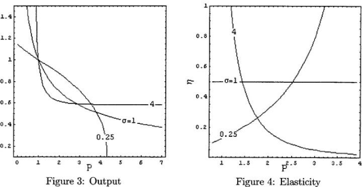
As stated earlier, our interest in estimating a stems from the fact that it determines

the quantitative effect that investment distortions have on per capita incomes. To illustrate this point we simulate the model for several values of a, and show how distortions affect

per capita incomes for each value of a. As it turns out, the impact of distortions under

a = 0.7 is significantly stronger (in a sense to be made precise below) than under a

=

1.

This improves the explanatory power of the neoclassical mo dei (to explain income gaps as coming from differential distortions) and suggests that policies that reduce distortions in

•

poor (highly distorted) countries are more effective than they would appear under a

=

1.0. '.

We also perform a development decomposition exercise â la Hall and Jones (1999) and show that the correlation between per capita income and TFP is smaller under a = 0.7 than under

a = 1.0. Finally, as an application of our estimation results, we assess what portion of the distortions that our model formulation is based on is refiected in the PWT.

The rest of the paper is organized as follows. Section 2 presents a theoretical model and derives the equation that is to be estimated. Section 3 describes the econometric procedures used for estimating this equation. The numerical results of our estimation are then reported and discussed in Section 4. Section 5 calculates the bias in the regression that would occur

if one were to ignore the country specific effects. Section 6 conducts quantitative exercises, illustrating how our estimation results are applied to the question of income gaps. Section 7

concludes.

2 Model Specification

2.1 Theoretical Model

We consider a two sector neoclassical growth model. Time is continuous and the horizon is infinite.

Sector 1 produces a consumption good, using labor and capital. The per capita output

Yl in this sector is

(1)

where II is the fraction of the labor force employed in sector 1, k1 is the capital-labor ratio

in sector 1, A is total factor productivity and

f

is the C.E.S. production function specified in (3).

4

•

Sector 2 produces an investment good, using labor and capital. The per capita output

Y2 in that sector is

(2)

where B is an investment sector productivity parameter. The function

f

is specified as

(3)

where (J" is the elasticity of substitution between capital and labor and Q: is a parameter

relating to income shares.

There is a continuum of identical, infinitely lived individuals in the economy that act as consumers, workers and owners of capital. The supply of labor of each individual is inelastic at 1 unit per unit time and there is no disutility from working. The measure of individuaIs is 1. Individuals take prices as.given and make intertemporal consumptionjsavings decisions, where savings are effected by buying capital goods and renting them out to firms.

There is a continuum of profit maximizing, price taking firms that buy inputs (labor and capital services) from individuals and seU output back to individuals.

The lifetime utility of a representative individual is

00 1-.1

J

e-pt-t-dt

c-r

1_1 '

o -y

(4)

where C_t is the date

t

consumption f1.ow. p is the subjective, instantaneous rate of time preference and I is the intertemporal elasticity of substitution.

Consider some fixed point in time, say

t.

Then at that point a representative individual receives the f1.ow wage of Wt and the f1.ow rental rate of qt per unit of capital good that she

rents out to firms. Let Pt be the price of the investment good. All prices are denominated in

terms of the consumption good, which is the numeraire commodity. Then a representative individual faces the foUowing budget constraints

(5)

where Kt is the individual's capital stock, It is the individual's addition to this capital stock,

The capital accumulation equation is

(6)

where 8 is the physical depreciation rate. The individual's initial endowment of capital is exogenously specified and denoted by Ko.

If we substitute (6) into (5) we get

•

PtKt - (qt - 8pt) Kt

=

Wt

+

Xt - Ct. (7)

It is convenient to introduce the interest rate

rt = qt - 8pt = qt _ 8.

Pt Pt (8)

Then, maximizing (4) subject to the budget constraints (7), one gets the Euler equation

(9)

•

We are going to focus on a steady state, where Ct = O and where investment is solely

used to replace depreciating capital.

To this economy we add "distortions" that come either from government policy or from non-economic considerations (cultural, historical and sociological features of real life economies). The effect of these distortions is to drive a wedge between the equilibrium prices that would have prevailed in their absence and the prices that agents (individuaIs and firms) actually face. To determine the prices that agents face, we first find the prices that would have prevailed in the absence of distortions. Then we tack on distortions to these prices.

As stated above, we focus on a steady state. Then equilibrium prices are time invariant. Since any input combination that produces one unit of the consumption good, produces B units of the investment good, the relative price of capital is

1

P= B·

Given this, the rental rate of capital is q = AI' (k), the interest rate is r = ABI' (k) - 8 and

the wage rate is W = A

[i

(k) - kI' (k)].

Next we consider distortions. The government imposes a tax on the investment good at

•

..,

•

the rate of TI or, alternatively, imposes a tariff on the importation of investment goods in

case the economy is open.1 _{In addition, the government imposes a tax on capital income}

at the rate of TK. An alternative interpretation of TK is that it is the fraction of earl1Íngs that organized crime extorts from owners of capital. Or TK maybe money that owners of capital must pay to corrupted government officials to be able to run their businesses (which, in effect, means that capital income is taxed). Whatever the interpretation of these tax rates, the investment tax and the capital income tax are returned to individuals in the form of lump sum transfers and appear as Xt in the individual budget constraints.

As a consequence of these distortions, individuals pay

Ti

1

+

TI

p=-::::::--B B

for the investment good, and receive

as net rental rate on capital.

q

=

AI' (k) :::::: (1 _ TK)Af' (k)

TK

Combining (8) and (9) we have that

r = Q _ 8 = AI' (k) 1 _ 8 = p

P T_K P ,

which implies

I TK

Ti

TK

f

(k) = Pil (p

+

8)

=

B

il

(p

+

8) . Now, since

f

exhibits a constant elasticity of substitution, (3) implies

k _

(f'

ｾ＠

k) ) - ( r

f

(k) '-<

Substituting (11) into (12), we get

k _ [TrTK P

+

8]

-u

f

(k) -

BA----;-(11)

(12)

(13)

Next we compute national income statistics at the steady state. The per capita GDP of

1 Considering an open economy requires slight notational modifications. However, the equation to be

the economy y is defined as

Y2

Y = Yl

+

B·

Using (1) and (2) and substituting the equilibrium condition for the labor market,

ir

+l2 = 1, we see that Y = Af (k), where k is the stock of capital per capita. Then, using the fact that the steady state investment, 8k, is equal to sector 2's output, ABld (k), the economy's

resource constraint is

Y

=

Af(k)

=

c+inv

=

c+

ｾＬ＠

(14)

where 'inv' is the per capita flow of investment goods (we reserve the letter i for the investment-output

ratio).

2.2 Taking the Model to Data

This completes the derivations of theoretical relationships that hold for a single economy. Let's consider now a cross section of economies, indexed by j. Each economy is characterized

by its own TFP parameter Aj, its own investment sector productivity parameter Bj, and

its own distortions TI,j and Ti<:.,j. To make consumption, investment and GDP comparable across countries we evaluate them in terms of international prices2 _{and, without loss of} generality, we let the international price of investment be one.3 _{Then, ifij is the steady} state investment-output ratio in country j, (14) tells us that

(15)

Substituting (13) into (15), the long run investment-output ratio is

(16)

Taking logarithms on both sides of equation (16), we get a log-linear relationship between the relative price of capital and the investment-output ratio

(17)

2The issue here is that the investment-consumption price ratios are not equal across countries. We handle this issue by adopting the procedure developed by Restruccia and Urittia (2001).

•

where

lnFEj

==

In

[8

ＨｐＺＸｔｾＬｪＩＢ｝＠

-

(1-

O")lnAj . (18)

F Ej is referred to as the jth economy fixed effect.

In Sections 3 and 4 we estimate the long run relationship (17). As stated in the intro-duction, several studies indicate that total factor productivity (A) and thus the fixed effect

(F E) is correlated with investment and output. In the language of our formulation, this may

come from correlations between A and

Tr

or B; it has been argued, for example, that high productivity economies happen also to be less distorted. It may also come from correlation between TK and

Tr

or B; for example, distortions to capital creation may be related to dis-tortions to capital remuneration. If such correlations exist, then the fixed effect is correlated

Ｇｾｲｩｴｨ＠ prices and if this correlation is ignored, the estimation results are going to be biased.

In estimating

(17)

we take the possibilty that such correlations exist into account.

Before we proceed to the estimation, we note that our results apply beyond the particular model we presented above. In particular, if there is population growth at the rate n and

disembodied, labor-augmenting technological progress at the rate g, equation (18) is replaced by

lnFEj = In [8EF (

ｾ＠

fl 71

1

.)(1]-(1-

0")

lnAj, p+

+

'"Y K,J

where

8EF

==

8

+

g+n.

Equation (17) remains intacto Then the estimation procedure is identical to the one we present here.

point of view.

3

Empirical Implementation

Our ultimate goal is to estimate the long run price elasticity of investment demand, i.e., the parameter O' in equation (17). Somewhat imprecisely, we also refer to O' as the price elasticity of demand for investment goods. Assuming that all countries share a common value for 0',

the investment demand is the same for all countries apart fram a country specific effect (or an "intercept"), which comes either from differences in TFP Aj or from the policyjinstitutional

variable, TK,j, or both. These country specific effects are subsumed in the fixed effect term (18). To account for these effects as well as to distinguish between short run and long run price elasticities, we employ (among other things) dynamic panel data techniques.

Dynamic panel data techniques are advantageous in our context for three reasons. First, the regression analysis relies on data that exhibit greater variability as compared to pure time series or pure cross section data. Second, panel data techniques allow us to identify country specific effects, which would have been impossible if we were to use pure cross section techniques. Third, using dynamic panel data techniques, we are able to distinguish between the short and long run price elasticities of demand for investment.

For completeness and to show the advantages of dynamic panel data techniques over more traditional methods, we work v.rith two econometric specifications. In the first static speci-fication, the lagged dependent and the lagged independent variables are not included on the RHS of the regression equation. In the second dynamic specification these lagged variables

are included. The next two subsections describe these specifications and the econometric

exercises that we perform on them.

3.1 Static Panel

Based on the theory above, see equation (17), we consider the following static specification of the demand for investment

In ijt = In F Ej

+

/3

₀ Inpjt

+

Cjt,

c jt '"" iid( 0,0';),

j

=

1,2, ... ,N, t=1,2, ... ,T,

(19)

l

•

-where In F Ej is an unobserved time invariant country specific effect, Cit is an error term, subscript j is a country index and subscript

t

is a time indexo Depending on the exercise (see below) the time period is either one year or an average over either 6 or 7 years. (30 is the same as u in Section 2.

If we use the original, annual data set, four issues need to be addressed. First, we need to determine whether to use estimation techniques that consider the country specific effect as a fixed-effect (FE) or as a random-effect (RE). Second, we need to account for the possibility that error terms are heteroskesdastic, i.e., that they have different variances for different countries. Third, we need to account for the possibility that the explanatory variable In Pjt

is correlated with the error term Cjt (the so called endogeneity issue). Fourth, we need to

test and correct for the possibility that error terms are serially correlated. We describe now how each of these issues is dealt with .

• FE versus RE. The FE mo deI is estimated by the Within Group estimator (WG). To do that we first average equation (19) over time to get the cross section equation

(20)

where In

tj -

_ｾ＠

2::=1

In ijt , lnpj

=

ｾ＠ 2::=llnpjt and Ej

=

ｾ＠

2::=1

Cjt. Second we

subtract equation (20) from (19) for each

t,

which gives a transformed equation. Third we run an OLS regression on the transformed equation. The RE model, on the other hand, is estimated by the GLS random effects estimator. This procedure is more involved so we refer the interested reader to Baltagi (1995), Chapter 2, where it is fully described.

Comparing the two procedures, the GLS random effect estimator is more efRcient, but it yields consistent estimates only if the country specific effects are not correlated with the regressors. On the other hand, the FE estimator is consistent regardless of the correlation between the country specific effects and regressors. To find out which estimator is more appropriate we apply a Hausman test to determine whether the difference between the estimated parameters according to these two procedures is small or large. If the difference is large, then we conclude that there is correlation between the country specific effects and the regressors, and we adopt the FE estimator .

been derived in Arellano (1987), is that it is robust to heteroskedasticity.4

• Correlation between the explanatory variable and the error terms. We relax the com-monly held assumption that lnp is strictly exogenous, which means that it may be

correlated with ê for some leads and lags. To account for that possibility, we let the lagged value of the regressor be an instrumento Then, to assess whether lnpit-l and

é jt are correlated, we apply the Sargan test of over identifying restrictiOllS.

• Serial correlation of error terms. Given that we use a static specification and that we work with annual data, it is possible that the error terms are serially correlated. Most notably, this may occur because relevant variables are omitted. To check for that, we apply a first order serial correlation testo If this test indicates the presence of serial correlation, one can remedy this by explicitly allowing for serial correlation. Qne commonly used remedy is to assume that error terms are AR(l) correlated

êjt = pêjt-l

+

l/jt,

l/jt '" iid(O, ＨｔｾＩＮ＠

(21)

Then under this AR(l) assumption the estimation procedure is carried out as follows. First, the AR(l) coefficient, p, is estimated using the residuaIs from WG estimation. After estimating p, the data is transformed and the AR(l) component is removed. Finally, the WG estimator is applied to the transformed data.

A potential problem with this remedy is that it is very limited. It assumes a particular form of serial correlation and it does not deal directly with the source of the serial corre-lation, namely the omission of relevant variables. We show these limitations below (see footnotes 8 and 9) by comparing the regression equation that an AR(l) transformation produces with the regression equation that one gets with a more general formulation, i.e., a formulation in which no variables are omitted.

AlI this describes the issues that arise if one uses the original annual data set. One way to get around these issues is to create a new, low frequency data set. This is done by averaging

4The formula for the consistent standard error of the WG estimator of fio is

N

var(fio) = (X'X)-l(2: Xjêjê;Xj)(X'X)-l,

j=l

where

X

j = In Pj -In fij , êj = (In ij -In lj) - fio(ln Pj -In fij ) and all bold face variables are T x 1 vectors.

As Arellano (1987) shows, this standard error formula is valid under the presence of any heteroskedasticity

or serial correlation in the error terms - as long as T is small relative to N.

the original data over (say) six or seven year disjoint time blocks. Then, one estimates the static equation

(19),

where each time period is one of these blocks. The downside of this estimation strategy is that it reduces the number of data points available as inputs into the regression analysis and thus reduces the efficiency of estimators.5 _{The upside is that} the estimates one gets are long run estimates (which is what we are interested in) and that

they are unbiased. Chirinko et aI. (2002) provide a detailed description of this 'averaging' estimation strategy. We pursue this strategy in our context and report estimation results for it.

An

alternative estimation strategy is to keep using the original annual data set but enrich the econometric specification to cope with the above four issues. Recall that our goal is to estimate the long run price elasticity of investment demando The problem we run into is that the data presents us with short run fiuctuations of the price of investment goods and with consequent short run adjustments to them. If we use the static specification

(19),

these short run adjustments introduce correlations between contemporaneous investment, the lagged values of investment, and the lagged values of prices. To cope direct1y with these correlations we abandon the static formulation

(19),

introduce a dynamic formulation into which these lagged values are integrated and then estimate the dynamic formulation. We describe this approach in the next subsection.

3.2 Dynamic Panel

The dynamic econometric specification is

In ijt

=

In F Ef

+ /31

In ijt-

1 + /32

1npjt

+

,83 lnpjt-1

+

Ejt, Ejt '"" iid(O, a;),

(22)

where In F Ef are unobserved time invariant country specific effects, superscript 'D' stands

for dynamic and Ejt are the error terms.6

5 Another commonly used approach in the macroeconometrics literature is to 'smooth' the data. That

approach however distorts the available information and has been widely criticized by econometricians. 6The dynamic specification (22) is related to the static specification (19) with AR(l) error terms as follows. Substituting (21) into (19), the AR(l) regression equation is wTitten as

where

---The parameter 13₂ in equation (22) is interpreted as the short run price elasticity of

investment demando The corresponding long run price elasticity is derived from (22) by setting Ejt

=

O, In i jt

=

In i jt-1 and solving the resulting relationship between In i and lnp. Then the long run price elasticity iS7

13_LR

=

LR(13_{1 ,} 132' 13_{3 )}

==

132

+

:3.

1- 1 (23)

Econometrically (22) is estimated via OLS and WG techniques, as in section 3.1, and also via Generalized Method of Moments (GNIl\II) techniques. For a detailed description of

GMM techniques see Chamberlain (1984), Holtz-Eakin, Newey and Rosen (1988), Arellano and Bond (1991), Arellano and Bover (1995), and Blundell and Bond (1998a).8

Applying GMM techniques to the problem at hand, we report estimation results following two approaches. In the first approach, which is based on Arellano and Bond (1991), country specific effects are eliminated by taking first differences of the regression equation.9 _Applying

this to (22), we get

In i jt -In ijt_1

=

131 (In ijt-1 -In ijt- 2)

+

132 (lnpjt -lnpjt-l)

+

133(lnpjt-l -lnpjt-2)

+

f.jt - Ejt-l·

(24)

Assuming that the Ejt'S are serially uncorrelated (i.e., that E(EjtEjs)

=

O for t =1= s), In ijt-s are

valid instruments in these first differenced equations if s

2:

2. Then using these instruments

we get the following T - 3 moment restrictions

Then, if we set ,6₁ = P , {32 = {3o, {33 = -t3_oP and InFEf = (1 - p) In FEj , this regression equation is

the same as (22). In general, however, (22) contains three parameters whereas (19) with AR(l) error terms contains only two. Therefore, (19) with AR(l) is a (very) special case of (22).

7 A limitation of the static specification (19) with AR(l) error terms is now revealed: It does not allow

one to distinguish between the short and long run price elasticities of investment demando By the equation in the foregoing footnote and by (23), both elasticities are equal to (3o. Indeed

6AR(1) = {32

+

,83 = {3o - t30P = {3

LR 1 - {31 1 _ P O·

8Details concerning how these GMM techniques are applied to the problem at hand are found in Appendix A.

..

E(ln ijt-s ( Ejt - Ejt-1»

=

o

for s

2

2 and

t

=

3, .... , T. (25)

Assuming furthermore that In p is weakly exogenous,10 we get additional moment restrictions

E(lnpjt_S(Ejt - Ejt-1»

=

O for s "22 and

t

= 3, .... ,

T.

(26)

Arellano and Bond (1991) developed a consistent estimator, which is referred to as GMM-DIF, for this first difference approach. This estimator works well when the instruments are highly correlated with the regressors. Blundell and Bond (1998a) show via Monte Carlo simulations that if (31 is dose to 1 (and in our case it is), then the lagged values of variables are weak instruments for the corresponding differenced variables, causing the asymptotic and the small sample performance of the GMM-DIF estimator to be poor.ll _{Blundell and Bond} also show that the GMM-DIF estimator of (31 exhibits a downward asymptotic bias and large standard errors in small samples.12 _{Furthermore, recent empirical work (See Blundell and} Bond (1998b), Loyaza, Schmidt-Hebbel and Serven (2000) and Bond, Hoeffer and Temple (2001» shows that the estimate of (31 under GMM-DIF is close to the estimate of (31 under WG estimation, which, as we discuss later, is biased downwards. This empirical work also points out that GMM-DIF estimators are inefficient, Le., the standard errors ofthe estimates are large.

To overcome these biases and imprecisions we pursue a second, 'system' approach, referred to as GMM-SYS (or extended GMM) estimation. This approach combines, in a system, regressions in differences with regressions in leveis, as in Arellano and Bover (1995). The work of Blundell and Bond (1998a) shows - theoretically and via Monte Carlo simulations-that the leveI restrictions under GMM-SYS are informative in cases where the first differenced instruments are not (even if (31 is large). In addition the empirical work mentioned above

lOThe assumption of weak exogeneity of lnpjt is that E(€js lnpjt)

=

O for s > t.

lI A1though the autocorrelation of the ln ijt series is sufficiently below 1 that we can reject the unit root

hypothesis (see below), lnijt are still positively and highly correlated, i.e., fJl is positive and 'large.' Because

of that, the instrumental variables for In ij,t-z, In ij,t-3,"" In ij,1 are weak instruments i.e., they are not

strongly correlatcd with the regressors, and this poses prohlems for applying the GMM-DIF estimator. 12Blundell and Bond (1998a) evaluate the performance of the GMM-DIF estimator via Monte Carlo simulations. In particular, they consider the pure AR(l) case

Yit = "7.;

+

aYit-l

+

Vit·

shows that standard errors under GMM-SYS are smaller than under GMM-DIF.

This GMM-SYS estimator works as follows. The instruments for the regression in dif-ferences are the lagged values of the corresponding leveI variables as before. Symmetrically, the instruments for the regression in leveIs are the lagged differences of the corresponding variables. These are suitable instruments under the additional condition that there is no correlation between the differences of the right hand side variables and the country specific effects, which is written as13

E((lllijt_1 -lnijt- 2)11lFEf)

=

O E((111Pjt-1-lnpjt-2)lnFEf)

=

O.

Thell, adding to this the stalldard condition that E((lll _{ijt- 1-l11 ijt- 2)fjt)}

=

O and E((lnpjt-1-lnpjt-2)fjt) = O, we get the follo\Ving additional moment restrictions14

E((1n i jt_1 -In ijt-2)(1nFEf

+

fjt)) = O for

t

= 3, .... , T,

E((lllPjt-1 -lnpjt-2)(11lFEf

+

fjt)) = O for

t

= 3, .... ,T.

(27) (28)

Another advantage of the system GMM over the first-differellce GMM estimator is that it allows us to study not only the time series relationship (between price and demand for investmellt) but also their cross sectioll relationship.15 In any event, we report estimation results for both GMM-DIF and GMM-SYS.

To assess the empirical results of GMM-DIF and GMM-SYS, we apply two specification tests proposed by Arellano and Bond (1991). The first specification test is the Sargan test of over identifying restrictions, which tests for the overall validity of the instruments. The second test examines the hypothesis that the fjt are not second order serially correlated. 16

13This assumption doesn't require that there is no correlation between the leveIs of Inpjt and In P Ef.

Instead, this assumption follows from the stationarity property

E(ln ijt+m InPEJ)

=

E(Inijt+nlnPEJ) for any m. and n,

E(lnpjt+m InPEJ)

=

E(lnpjt+n InPEJ) for any m. and 11.

14Arellano and Bover (1995) show that further lagged difIerences would result in redundant moment restrictions if alI available moment restrictions in first difIerences are exploited.

15The GMM-DIF estimator eliminates the unobserved fixed efIects, while regression in leveIs does noto 16By construction, it is likely that E((éjt - éjt-l)(éjt-l - éjt-2)) i= O. Thcrefore, even if the original error

•

We also test the validity of the additional instruments in the leveI equations. The set of instruments used for the equations in GMM-DIF is a subset of that used in GMM-SYS, so a test of these extra instruments is naturally defined. We apply a "difference" Sargan test by comparing the Sargan statistic for the GMM-SYS estimator and the Sargan statistic for the corresponding GMM-DIF estimator.

Measurement Error. So far we assumed that variables are measured without errors. Measurement errors are not unlikely for our data set but, fortunately, our procedures are easily extended to cope with them. Specifically, suppose that In ijt and lnpjt are not directly

observed and that instead we observe

In i jt = In ijt

+

m;t, (29)

1 -_npjt -1 _{- npjt}

+

_mjt, p

where m;t and m;t are measurement errors that are uncorrelated with all of In ijt and In Pjt

and that are uncorrelated over time. Then, if one substitutes In ijt and lnpjt from equation

(29) into equation (24), one gets

-_{€jt -} -_{€jt-1 = €jt - €jt-1}

+

i i B(i i )

m jt - mjt-1 - I 1 m jt- 1 - mjt-2

- f32(mIJt

- m}t-1) -

f33(m}t-1

- mIJt-2)'

By the condition that the measurement errors are uncorrelated over time,17 we obtain the follO\ving moment restrictions

E(ln ijt-s(Jjt - Ejt-1))

=

O for s ｾ＠ 3 and

t

=

4, .... , T,

E(lnpjt_s(Jjt - Ejt-1))

=

O for s ｾ＠ 3 and t

=

4, .... , T,

E((lnijt_2 -lnijt-3)(1nFEf

+

Ejt))

=

O for

t

=

4, .... ,T,

E((1npjt-2 -lnpjt-3)(1nFEf

+

Ejt))

=

O for

t

=

4, .... , T.

terms are not serially correlated, the differenced error terms are, which means that the hypothesis that they

are not serially correlated would likely be rejected.

17 Alternatively, we could assume that measurement errors follow a moving average process of order l.

Once we have these moment restrictions we apply GMM estimation, following the same steps as before. Specification tests for the validity of the instruments are analogous too.

4

Data and Results

The data we use comes from the Penn World Table, PWT 6.0 (Heston et aI. 2002). To

balance the data, we extracted a sub-sanlple of 113 countries, observed over 37 years, from 1960 to 1996. TabIe 1 at the end of the paper lists all the countries in our sampIe. The relative price of investment that we use is the ratio of the 1996 international price leveI of investment, PWT variable pi, and the 1996 international price leveI of consumption, PWT variable pc. The investment-output ratio is the investment share of real GDP per capita evaluated at 1996 international prices, P\VT variable ki.

\Ve also constructed two 'average' panel data sets, derived from the above raw data. In the first paneI we averaged the data over six disjoint time blocks with six years in each block: 60-65,66-71,71-77,78-83,83-89, and 90-95. Each block tis considered one time period and we have si.'\: time periods altogether, T = 6. In the second panel we averaged the data over five disjoint blocks with seven years in each block: 60-66, 67-73, 74-80, 81-88 and 89-96. Then we have five time periods altogether, T = 5.

As a first step we checked whether the In ijt and the lnpjt series are stationary. To do

that, while accounting for possible trends we ran the regressions

In ijt - 80

+

8I

t

+

PIln ijt-I

+

Vjt

lnpjt 82

+

83t

+

P2 ln pjt-1

+

f.1jt,

using the STATA module xtdftest.18 _{Based on these regressions we test for stationarity,}

using the Fisher version of the Dickey-Fuller test under the assumption of no cross country correlation among the errors. We have chosen the Fisher test because, as shown in Madalla and Kim (1998), it is more robust than other tests to violations of the no correlation as-sumption. Applying this test we find that non-stationarity is rejected, Le., we reject the hypotheses PI

=

1 and P2 = 1. Therefore our sedes refiect stationary fiuctuations around

(perhaps) a deterministic trend. This allows us to proceed with the statistical procedures below.

Having done that, we present estimation results for the price elasticity of investment demando As a matter of convention, our estimates are discussed as positive numbers, which

18We thank Luca Nunziata for kindly providing us with this module.

means they should be interpreted as the absolute values of the actual elasticities (the tables report them as negative numbers). The overalI condusion that emerges from our analysis is that the estimates of the long run price elasticity are, for the most part, between 0.5 and 1. They tend to equal 1 when country specific effects are ignored and this is true regardless of whether we use static or dynamic panel techniques and whether we control for the endogeneity of the regressor (price) or noto At the other end of the spectrum, the estimates tend to be dose to 0.5 when country specmc effects are taken into account

but when serial correlation or, more generally, dynamic linkages are ignored. When both dynamic linkages aud country specmc effects are controlled for, then, depending on the particular procedure we use, the estimates falI somewhere between 0.5 and 1, and in the majority of cases are dose to 0.7. The order of presentation of these estimates folIows the order of presentation of the econometric specifications in Section 3.

4.1 Static Panel

4.1.1 Annual panel data

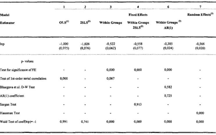
Table 2 reports estimation results for the static specification (19), using our raw almual data. 19 In column [1] we report the results of an OLS regression and in column [2] the results of a 2SLS regression. Both regressions do not control for country specific effects. The first regression ignores price endogeneity as well, while the second regression does noto As can be seen, the estimated price elasticity in columns [1] and [2] is around 1. Whether we control or do not control for price endogeneity, the Wald test does not reject the hypothesis that the price elasticity

=

1. This result agrees with the results of Restruccia and Urittia (2001) who, likewise, do not controI for country specific effects.

These results change dramatically when country specific effects are controlIed for. This can be seen in columus [3]- [7], which report regression results when fuced effects are (poten-tially) different across countries. The reported estimates in these columus are all well below 1, and actually dose to 0.5. In particular, the WG regression [3] yieIds price elasticity of 0.522 and, correcting for price endogeneity in column [4], we get a slightly higher estimate, 0.558. The Sargan tests of over identifying restrictions for the 2SLS regressions, columns [2] and [4], do not indicate a problem with the validity of instrumental variables.

In column [6] we check for first order serial correlation, AR(I), of the error terms -continuing to control for country specific effects (Le., running a WG regression). \Ve find

19 Ali results in Tables 2,3,4 and 5 are computed using Stata 7.0. The test of first order serial correlation

strong and positive serial correlation. The estimated AR(l) coefficient pis high, 0.725, and the Bhargava et aI. (1982) Durbin Watson test rejects p = O. The estimate of the price elasticity in this column, 0.385, appears excessively low. Recall however that when error terms are AR(l) correlated, the short and long run price elasticities are constrained to be equal (see footnote 9). Since the short run elasticity is smaller than the long run elasticity we interpret this estimate for (30 as an average between the short and long run elasticities. A more satisfactory approach obviously is to explicitly distinguish between the short run and long run elasticities in the econometric specificatioll, which we do below.

Column [7] of Table 2 reports regression results when country specific effects are treated as random effects, Le., when equation (19) is estimated via GLS with random effects. The estimate we get then, 0.566, is sufliciently different from the WG estimate we get under a fixed effect treatment, 0.522. Because of that the Hausman test rejects the hypothesis of no correlation between the fixed effects and the regressors. Consequently, we consider country specific effects as fixed effects from this point onwards.

The net result from all this is that working with the static specification and with annual data is inappropriate. Error terms are serially correlated, when we naively correct for them via AR(l) we get excessively low estimates of the price elasticity, and short run and long run elasticities are not distinguished. This suggest we should consider either transformed data or an alternative specification. vVe first present results for transformed (Le., averaged) data. Then we present results for the dynamic specifications.

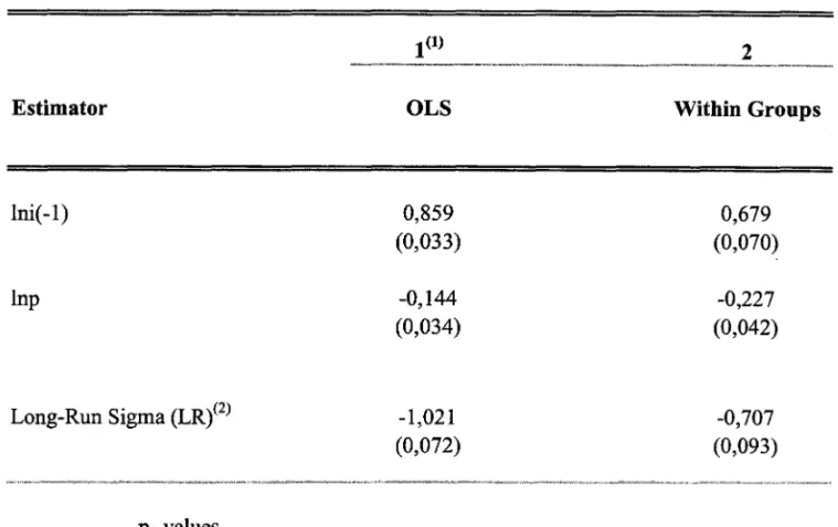
4.1.2 Average panel data

Table 3 presents the results for the 6 and 7 year average panels. The first thing to note here, see columns [1], [2], [5], and [6], is that, whell the fixed effect is cOIh<;trained to be equal across countries, the price elasticity is still around 1. Therefore averaging the data may (and as we shall see, does) remedy for serial correlation, but it is no panacea for ignoring country specific effects. The second thing to note is that the estimates in the remaining columns are larger than the corresponding estimates in Table 2 but are still significantly lower than 1. And the third thing to note is that accounting for price endogeneity here makes a bigger difference than in Table 2, i.e., it increases the estimates by a bigger margin. In the end, when we control both for country specific effects and for price endogeneity, we get 0.650 for the six year average (column [4]) and 0.674 for the seven year average (column [8]).

Another thing we did was to check whether the addition of a time variable makes a difference. To do that we re-ran the previous regressions with time dummies. The results are shown in Table 4. As this table shows, if we do not control for the fixed effect or for price

endogeneity (columns [1] and [5]), the estimated elasticity is still 1 and the dummies are significant. On the other hand, when we control for price endogeneity but not for country specific effects, only one time dummy is significant (columns [2] and [6]). The "VG estimates (columns [3] and [7]) without controlling for price endogeneity deliver values for

f3

₀ very dose to columns [3] and [7] of Table 3 and likewise columns [4] and [8] are similar in the two tables. Furthermore, the "VG estimates that control for price endogeneity (columns [4] and [8]) indicate that price dummies are insignificant. Finally the Wald Tests rejectsf3₀ = 1 in columns [3], [4], [7] and [8]. AlI in alI, the addition of time dmnmies makes little difference, especially when controlling for cross country heterogeneity and price endogeneity.

In summary, if we had to pick one estimate to report from this averaged panel exercise it would be the one for the six year average (column [4]), 0.66, with a robust standard error of 0.16; the corresponding estimate for the 7 year average has a higher robust standard error so we consider it inferior. The good news about this estimation strategy is that we get estimates of the long run elasticity and that serial correlation tests come back negative. Moreover, time dummies are significant only when we do not controI for price endogeneity. The downside is that alI standard errors are higher when we work with the averaged data than with the annual data. In particular, the WG-2SLS robust standard errors are doubled, compare columns [4] in Tables 2 and 3. This comes from the fact that we have less data points to work vvith when the data is averaged. AIso, this approach does not make a distinction between the short run and long run price elasticity of demando The approach we turn. to next makes this distinction.

4.2 Dynamic Panel

We implemented the dynamic panel specification, (22), employing OLS, \VG and GMM estimators. Before we comment on the numerical results we obtained, we discuss several issues that GMM estimation brings up. In particular we discuss what estimates we report, how we obtained these estimates and how one should goabout interpreting them.

The first issue to be discussed is that the usual GMM procedure that uses all lagged values as instruments becomes computationally infeasible when T gets large. This is shown

in full detail in Arellano and Bond (1998). Furthermore, Monte Carlo experiments (see Judson and Owen (1996)) indicate that increasing the number of instruments used creates a trade off. On the one hand, it increases the efficiency but, on the other hand, it increases the bias of the estimated

f3

_{1 •}20 _{To deal with this issue, we used a "restricted GMM" procedure}

in which the number of lagged values used as instruments was at most two.

The second issue is that we had to decide whether to report numbers from the one step or the two step GMM (we describe these procedures in Appendix A). The one step GMM is pred-icated on the error terms Ejt being independent and homoskedastic - both cross sectionally

and over time. But then standard errors and test statistics are not robust to heteroskedas-ticity. The two step GMM remedies this problem by constructing a consistent estimate of the variance-covariance matrix of the moment conditions (based on first step residuaIs) and then re-running the estimator.21 _{The problem with the two step GMM estimator however is} that the standard errors it produces are biased downward in small samples.22 _{This problem} is pointed out in Blundell and Bond (1998a). The same authors also show - via Monte Carlo simulations - that the precision of the one step GMM is not much lower than the precision of the two step GMM. Following up on these findings, we report the following estimates. For the point estimates of (J's we report the estimates from one step Gl\!Il\1; for standard

errors we report the estimates from one step GMM - corrected by the variance-covariance matrix computed from the first step residuals; and for specification tests and checking for second order serial correlation we report the estimates from two step GMM. This last choice is guided by the fact that the Sargan test, based on the two step GMM, is the only one that is heteroskedasticity consistent. Also, the asymptotic power of the second order serial correlation test increases in the efficiency of the GMM estimator,23 and the two step GMM is more efficient.

A third issue is whether to include lagged price lnpjt-l on the right hand side of the regression equation. As far as the generality of econometric procedure, lnpjt-l should be included.24 As far as economic theory, In pjt-l should be excluded. This is because a price shock in period

t

-

1 affects investment in period

t

-

1, In ijt-l' and In i jt - 1 affects In ijt. However, once this chain of effects is accounted for, there is no further, independent effect of

lnpjt-l on ln ijt. Nonetheless, and for completeness sake, we report estimation results both when lnpjt-l is included and excluded.

Let us now discuss now how to interpret the estimates, Le., which of the various estimates

21 If the error terms are spherical (homoskedastic), the one step and the two step GMM estimators are

asymptoticallyequivalent for GMM-D1F. Otherwise, the two step GMM is more efficient.

22Windmeijer (2000) created a procedure to correct the standard errors of the two step GMM estimator and embedded it into the DPD98 program for Gauss. He has kindly provided us with this procedure. We

applied it to our problem and the standard errors \V"B got were similar to those we got by correcting for

heteroskedasticity.

23See Arellano and Bond (1991).

241n order to pin down the correct specification one should start with a broad specification then let the statistical results dictate which V"ariable(s) to keep.

we report (OLS, "\VG, GMM) in Table 5 is more reasonable. As Nickell (1981) and, more recent1y, Blundell and Bond (1998a) show, the transformation underlying WG estimation (see Section 3) biases the estimated coefficient

131

downwards.25 _{Furthermore, standard}

results - in simpler settings - show that, when variables are omitted, the estimate of

13

₁ is biased upwards under OLS regression; Appendix C extends these results to our setting. As far as GMM estimation, it is known that if Tis small relative N, then GMM estimators are consistent, whereas WG estimators are noto In our case however T is not so small relative

to N (T

=

37, N

=

113) and theoretical results comparing Gl\1M and WG in this case are

just starting to emerge. The first such result is found in Alvarez and Arellano (2002). They consider the case where T / N tends to a positive constant and show that WG and GMM

estimators exhibit negative asymptotic biases.26 _{However, they also report several Monte}

Carlo simulations where T ::; N, and where the bias of the GMM estimator is always smaller than the bias of the WG estimator. Therefore even if N and T are of (approximately) the

same order of magnitude, it seems that GMM estimation is less biased.

Now we are ready to discuss the numerical results for the dynamic panel, as shown in Table 5.27 _{Odd numbered columns report estimates when}

Inpjt-1 is included on the RHS

of the regression equation, and even numbered colunms report estimates when Inpjt-1 is excluded. As can be seen, the coefficient of Inpjt-1 is not significant in columns [5] and [7]. The first four columns of Table 5 report OLS and WG estimates of the parameters

13

1 ,

13

2 and

13

3 together with estimates of the robust standard errors. As discussed above, the

OLS estimates of

131

are biased upwards while the vVG estimates are biased downwards.28

Computing the long run price elasticity

13

_LR from OLS estimation, we find that we cannot reject the hypothesis that it equals L

Colunms [5] to [8] report the results of GMM estimation. In all GMM regressions we take the conservative approach of allowing for measurement errors that are uncorrelated across time. The validity of the lagged leveI variables t - 3 and t - 4 as instruments in the GMM-DIF equation [5] is not rejected by the Sargan tests. Likewise the t - 3 lagged leveI variables combined with t - 2 lagged first differenced variables as instruments in GMM-SYS in [7] is not rejected by the Sargan tests. Similar statements apply to regressions [6] and [8]

25They show this however for the "pure" AR(l) case without exogenous regressors.

26 However, Alvarez and Arellano (2002) show this result for a first-order autoregressive model AR(l) without explanatory variables, with homoskedasticity and only the one step GMM estimator is considered.

27 AlI results in Tables 5, 6, and 7 are computed using the DPD98 software for GAUSS. See Arellano and Bond (1998).

where lnpjt-1 is not included as an explanatory variable.29 We have tested for second order

serial correlation and rejected that possibility.

As stated earlier, the WG estimates of (31 are known to be biased downwards. Columns [5] and [6] show that GMM-DIF estimates are smaller yet. 80 this suggests that the instruments used in the GMM-DIF estimator are indeed weak.

Interpreting the overall message of Table 5, we would say that estimates under GMM-8Y8, columns [6] and [8], seem the most reasonable. The estimated coefficients of In ijt -1 are

higher than the WG estimates, which are knOWIl to be biased downwards, and lower than the • OL8 estimates, which are known to be biased upwards. Furthermore, the estimated

coeffi-cient of In ijt _ 1 under GMM-DIF is lower than under \VG, so the GMM-DIF procedure seems to go in the wrong direction. If we compare standard errors, there is a gain in precision from exploiting the additional moment restrictions. And, finally, the difference 8argan statistic that tests the additional moment restrictions confirms their validity. Comparing colunms [7] and [8] suggests that lnpjt-1 can be omitted. Therefore, if we consider regression [8] as the most reasonable, the coefficient on the lagged dependent variable is 0.744, the short run price elasticity is 0.177, and the two together imply a long run price elasticity of investment demand of 0.691 (0.174). We tested the hypothesis that the long run price elasticity is 1, and rejected it at the 10% significance leve1.3o

Although the estimates reported under [8] seem the most reasonable, it is worth noting that the point estimate for (3LR from \VG estimation, regression [4], is very dose to the point estimate from the GMM-8Y8 estimation, colunm [8]. Although the WG estimation results are biased, Nickell (1981) shows that this bias is of ｯｲ､･ｲｾＮ＠ Therefore, since T is fairly large in our data set, this bias is quantitatively small. Note also that WG estimation rejects

f3

LR = 1 at the lower, 5%, significance leveI.

In Table 6 we report OL8 and WG estimates for the dynamic specification with time dummies added to the RH8 of the regression equation.31 We obtained very similar results to those in Table 5 (columns [2] and [4] respectively). In particular, the vVG estimation

291n this case, we use the lagged leveI t - 2 as instruments in the first-differenced equation (24). AIso we use t - 2 as instruments in the first-differenced equations, combined with lagged first-differenced variables dated t - 1 as instruments in the leveI equations in (22) for lnp.

30The standard error of {3LR is obtained by using the Delta method. See appendix B.

31 As before, it was infeasible to apply Gl'vfM estimators when time dummies are included. This is

because the total number of instruments would then be excessively large relative to the cross section dimensiono This implies that the two step GMM estimator, cannot be computed because the matrix

lV

W2

=

(ir

I:

Zf'EjEj'Zf)-1 is not invertible. See appendix A and,. for a full treatment of invertibility j=1

indicate long run price elasticity of investment demand of 0.707 (0.093).

For completeness we tried a more general lag structure of the dynamic specification, which includes a second lag of the price and investment variables. The last two columns of Table 7 report GMM-SYS estimations of this generalized equation. It turns out that both lagged variables In ijt-2 and In pjt-2 are not significant.

What we can say as an overall summary from this analysis is that putting lagged invest-ment on the RHS of the regression equation shows a positive and significant coefficient (31 and eliminates the need to add an arbitrary serially dependent error term.32 _{In addition it} allows us to distinguish between the short run and long run price elasticities and, as it turns out, this distinction is quantitatively significant; the long run price elasticity of investment demand is more than three times bigger than the short run elasticity.33 And finally if country specific e:ffects are not controlled for, we continue to get a long run estimate of 1 even with dynamic panel data techniques.

5 The Bias of OLS Estimation

A repeatedly appearing result in Section 4 is that, when country-specific effects are ignored, the Cobb-Douglas hypothesis (j = 1 is accepted. In this section we investigate what gives

rise to this resulto We do this by calculating the bias that comes from not considering country specific e:ffects and adding this bias to the estimated value of (j when these e:ffects

are considered. Then the sum of the two is indeed l.

To begin with, let's define

i' - ＨｩｾＬ＠

... ,ij, ... ,i:V)

whereij:::(ij1, ... ,ijt, ... ,ijT) and

p' - ＨｰｾＬ＠

... ,pj, ... ,p:V)

wherepj=(pj1'··',Pjt"",PjT).

The variance-covariance matrix of the PWT data is

M = [ var (In i) cov (ln i, In p) ] = [0.605 -0.307]. cov (In i, In p) var

(In

p) -0.307 0.306

32Note that the estiroated value oi 131,0.744, is quite close to the estimated p that we obtained with the static AR(l) specifications, 0.725.

33We also conducted a wide array of sensitivity analyses to verify the robustness oi OUl" results. First,

Then the OLS estimate of the static panel satisfies

ílOLS _{= -1 00 = cov (In i, lnp)}

=

_{cov ((lnFE}

+

_{f30 In p) , lnp)}

=

_{cov (InFE, lnp)}

+

_f3

o . var

(In

p) var (In p) var (In p) o·

This implies that OLS estimation wilI bias upwards the estimated value of _f30 whenever cov(ln FE, In p)

<

O (which, as the next paragraph shows, is the case).

An

analogous - although more involved - proof applies to the dynamic paneI. In Appendix

C,

using the fact that var(ln p)

ｾ＠

-cov(ln i, In p)

ｾ＠ ｾｶ｡ｲＨｬｮ＠

i), that

íl3

=

íl3,Bias

=

O

and assuming that alI economies are on a balanced growth path in the first period, we show that

ô

7PLS ,uLR ôcov (In

F'E

D , In p)

ｾｏｌｓ＠

íl2

+

íl2

Bias

>

O, where f3LR = _

(7' .:.. ) .

1 f31

+

f31,Bias

(30)

Thus OLS estimation biases upwards the estimated value of f3LR for the dynamic panel as welI. Furthermore, using the estimated values of var(lnFED) and cov(lnFED,lnp), we

ｾｏｌｓ＠

calculate _f3LR directly, obtaining 1.04.34 This helps explain why ignoring country specific effects biases the estimate of f3 upwards and leads to the erroneous condusion that the

aggregate production function is Cobb-Douglas.

To further substantiate this result and relate it to previous literature, we have done the following exercise. We restricted our time averaged data set to the more or less homogeneous set of 15 OECD economies. Table 8 displays estimation results for this sub panel when cOlmtry specific effects are ignored. As shown in that table, the price elasticity estimates we get for _f30 are between 0.54 (for 6 year averaging) and 0.76 (for 7 year averaging).35 These results are what we had expected. VV11en attention is restricted to a small set of similar countries, country specific effects are approximately the same. Then the estimates we get should be dose to the ones we get when we consider a large set of dissimilar countries, but when country specific effects are controlIed for. This result is also in conformity with results reported by ColIins and vVilliams (1999), using a similar approach, i.e., restricting attention to OECD economies.

To illustrate what country specific effects add to the statistical quality of results, we

,

_D (-D )

34This estimate is obtained by computing var(lnFE ) cov lnFE ,lnp (which falI out ofthe estimation)

ｾｏｌｓ＠

and from them get /3LR directly. Note that this direct estimate is not far of! the estimate we report in Table 5, column 2.

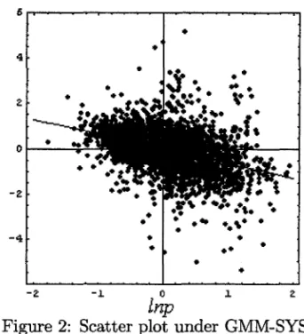
present the scatter plots of

(A I nz_ .

=

In ijt -

'131

In ijt -ｾ＠

1

-

In

FJjjD

j , I . .) npJ

1 -

/3

1 _{t=1, ... ,36 N=1, ... ,113}

Figure 1 shows this scatter plot for OLS estimation and Figure 2 shows it for GMM-SYS estimation. These Figures show that the scatter plot is tighter around the regression line for GMM-SYS, giving us a better fit of the data when country specific effects are included.

6

•

•

...

'

.

•

_•

4 ••• 4

•

_•

•

2 2

....

_•

_•

s;:: o o

<

-2 -2

•

-4 -4 •

•

•

• •

•

•

..

_•

_•

•

••

•

-2 Ｍｾ＠ o ｾ＠ 2: -2 Ｍｾ＠ o ｾ＠ 2

inp

_lnp

Figure 1: Scatter plot under OLS Figure 2: Scatter plot under GMM-SYS

6

Quantitative Exercises

In this section we perform several quantitative exercises, showing what bearing our estimation results have on several important issues of economic development and income gaps across countries. In Subsection 6.1 we make the point that ifwe compare our estimated u, u

=

0.7,

to the traditionally used u, u

=

1, then our u magnifies the effect of distortions and thereby

raises the neoclassical model's capability to explain income differences. In Subsection 6.2 we perform a development decomposition exercise à la Hall and Jones (1999). This exercise suggests that u

=

0.7 reduces the correlation between TFP and per capita incomes and