Affiliation, Equilibrium Existence and the
Revenue Ranking of Auctions
∗
Luciano I. de Castro
†First version: January 2004
This version: February 20, 2007
Abstract
We consider private value auctions where bidders’ types are dependent, a case usually treated by assuming affiliation. We show that affiliation is a restrictive as-sumption in three senses: topological, measure-theoretic and statistical (affiliation is a very restrictive characterization of positive dependence). We also show that af-filiation’s main implications do not generalize for alternative definitions of positive dependence.
From this, we propose new approaches to the problems of pure strategy equi-librium existence in first-price auctions (PSEE) and the characterization of the rev-enue ranking of auctions. For equilibrium existence, we slightly restrict the set of distributions considered, without loss of economic generality, and offer a complete characterization of PSEE. For revenue ranking, we obtain a characterization of the expected revenue differences between second and first price auctions with general dependence of types.
JEL Classification Numbers:C62, C72, D44, D82.
Keywords: affiliation, dependence of types, auctions, pure strategy equilib-rium, revenue ranking.
1
Introduction
What is the auction format that gives higher expected revenue when bidders’ types are dependent? This is an important question, made in a realistic context. Dependence of private information is more realistic because there are many sources of correlation of opinions and assessments in the real world: education, culture, evolution, common
∗I am grateful to seminar participants in 2006 Stony Brook Game Theory Festival, Washington University,
University of Paris I, Universidad Carlos III, Universidad de Santiago de Compostela, University of Illinois, Universitat Pompeu Fabra, Penn State University and to Aloisio Araujo, Alain Chateauneuf, Maria ´Angeles de Frutos, ´Angel Hernando, Humberto Moreira, Paulo K. Monteiro, Andreu Mas-Colell, Sergio Parreiras and Jeroen Swinkels for helpful conversations. I am especially grateful for Flavio Menezes’ comments and suggestions. Find updated versions of this paper at www.impa.br/∼luciano. Comments are welcome.
†Department of Economics, Carlos III University. Av. Madrid, 126, Getafe - Madrid, Spain. 28903.
sources of information, etc. Moreover, independence is a “knife-edge” assumption. The importance of the revenue ranking of auctions can be seen by realizing that it is a practical version of the main problem of mechanism design — what is the best mechanism for a decision maker (in this case, the seller)? We say that it is a “practical version” because it differs from the general one in restricting the set of considered mechanisms to the auctions most observed in practice (English auction and first price auctions).
In fact, the revenue ranking of auctions is a problem as old as auction theory itself. Among the many questions addressed by Vickrey (1961), this was one of most central-ity. His celebrated Revenue Equivalence Theorem (RET) says that the two above cited auctions (and his second price auction) give exactly the same expected revenue. Never-theless, RET requires independence of private information (types). Thus, the revenue ranking of auctions with dependent types remained unknown.
The best contribution to this matter was made through a remarkable insight of Mil-grom and Weber (1982a), which introduced the concept of affiliation in auction theory.1
Affiliation is a generalization of independence — see the definition in subsection 3.2 below — that was explained through the appealing notion that our assessments of values are positively dependent: “Roughly, this [affiliation] means that a high value of one bidder’s estimate makes high values of the others’ estimates more likely.” (Milgrom and Weber (1982a), p. 1096.)
Among the many interesting results in Milgrom and Weber (1982a), we underline the following:
• affiliation implies the existence of a symmetric, increasing, pure strategy equi-librium for first price auctions;2
• under affiliation, the English and the second price auction have higher expected revenue than the first price auction.3
In the face of these results, it is possible to cite at least three reasons for the deep influence of the aforementioned paper in auction theory: (i) its theoretical depth and elegance; (ii) the plausibility of the hypothesis of affiliation, as explained by a clear economic intuition; (iii) the fact that it implies that English auctions are better for
1In two previous papers, Paul Milgrom presented results that use a particular version of the same concept,
under the name “monotone likelihood ratio property” (MLRP): Milgrom (1981a, 1981b). Before Milgrom’s works, Wilson (1969 and 1977) made important contributions that may be considered the foundations of the affiliated value model. Nevertheless, the concept is fully developed and the term affiliation first appears in Milgrom and Weber (1982a). See also Milgrom and Weber (1982b). When there is a density function, the property had been previously studied by statisticians under different names. Lehmann (1966) calls it Positive Likelihood Ratio Dependence (PLRD), Karlin (1968) calls it Total Positivity of order 2 (TP-2), and others use the name Monotone Likelihood Ratio Property (for the bivariate case).
2They also proved the existence of equilibrium for second price auctions with interdependent values.
In our set-up (private values), the second price auction always has an equilibrium in weakly dominant pure strategies, which simply consists of bidding the private value. Although equilibria in mixed strategies always exist (Jackson and Swinkels 2005), first price auctions may fail to possess a pure strategy equilibrium when types are dependent.
3For private values auctions, which we consider in this paper, English and second price auctions are
sellers, which is a good explanation for the fact that English auctions are more common than first price auctions.
Nevertheless, since we were originally interested in the general problem of depen-dence of types, it is important to have an assessment of how strong as assumption affiliation is and how far its implications go.
In section 3 we show that affiliation is quite restrictive in three senses. It is re-strictive in atopological sense: the set of no affiliated probability density functions (p.d.f.’s) is open and dense in the set of continuous p.d.f.’s. It is also restrictive in a
measure-theoreticsense: ifµis a probability measure over the set of joint probabilistic density functions (p.d.f.’s), and ifµsatisfies some reasonable conditions, then thenµ
puts zero measure in the set of affiliated p.d.f.’s.
Finally, we argue that affiliation is restrictive in a statistical sense. Recall that affiliation was introduced through the intuition of positive dependence. In Statistics, there are many definitions of positive dependence and affiliation is just one of the most restrictive. Moreover, in sections 4 and 5 we show that the main implications of affilia-tion — equilibrium existence and the revenue ranking of aucaffilia-tions — do not extend for other (still restrictive) definitions of positive dependence.
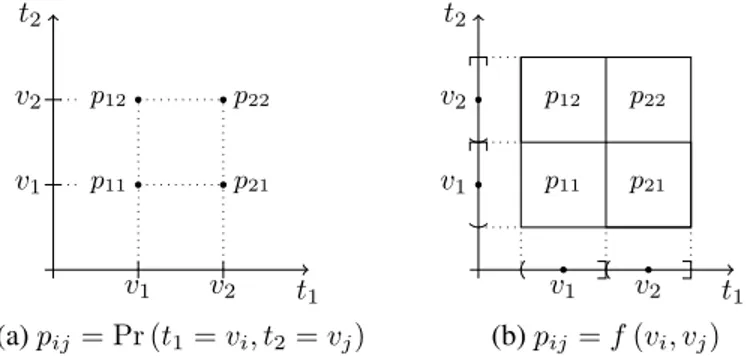
From this, it seems important to reconsider the problems of equilibrium existence and revenue ranking of auctions with dependent types. For solving the problem of symmetric increasing pure strategy equilibrium existence, we restrict the set of dis-tributions considered. The idea is so simple that it can be explained graphically (see Figure 1).
t1
t2
v1 v2
v1
v2
p11 p21
p12 p22
(a)pij= Pr (t1=vi, t2=vj)
p11
p12
p21
p22
t1
t2
v1 v2
v1
v2
(b)pij =f(vi, vj)
Figure 1: Discrete values, such as in (a), capture the relevant economic possibilities in a private values model, but preclude the use of calculus. We use continuous variables, but consider only simple density functions (constant in squares), such as in (b).
richness in the set of distributions, we focus in the set of densities which are constant in some squares around fixed values. This imposes no economic restriction on the cases considered, but allows a complete characterization of symmetric increasing pure strategy equilibrium (PSE) existence (see subsection 4.2).
It is easy to see that, as we take arbitrarily small squares, we can approximate any p.d.f. (including non-continuous ones). Thus, even if the reader insists on mathematical generality, that is, to include other distributions, our results are still meaningful because they cover a dense set.
For this set of simple p.d.f.’s, we are able to provide an algorithm, implementable by a computer, that completely characterizes whether or not a pure strategy equilibrium exists. Theoretical results are also available.
The results in section 4 reveal that the set of affiliated distribution is small even in the set of distributions with a PSE, sharpening the results of restrictiveness of affilia-tion. On the other hand, the proportion of p.d.f.’s which has PSE is also small. We offer a mathematical proof of this fact. This suggests that most of the cases only have equilibria in mixed strategies.
From this, we consider the characterization of the revenue ranking of auctions. The standard approach in the literature (see Milgrom and Weber 1982 for affiliated distribu-tions and Maskin and Riley 2000 for asymmetrical independent distribudistribu-tions) is to give conditions on the set of distributions that imply such or such ranking. Unfortunately, the conditions are usually very restrictive.
Numerical simulations, made possible by the results of sections 4 and 5, suggest that a complete characterization is very difficult. Even p.d.f.’s with positive dependence may often present a revenue ranking contrary to that implied by affiliation.
From this, we see two options for approaching the problem of revenue ranking. One is to obtain (experimental or empirical) information related to the specific situation and restrict the set of p.d.f.’s to analyze. Then, with this restriction, use our model to run simulations and determine what auction format gives higher expected revenue in the specific environment. Although this kind of “engineering” approach was recently proposed by Roth (2002) as a tool for economists, it will be useful to also have a general, theoretical model. This is the other part of the proposal.
We construct a “natural” measure over our proposed set of p.d.f.’s — this is natural in the sense that it comes from the limit of Lebesgue measure over finite-dimensional sets and also has some (partial) characteristics of Lebesgue measure. Using this mea-sure, we obtain an “expected value” of the expected revenue difference of the second-price and the first-second-price auction.
We illustrate this theoretical (and specification-free) method in section 5. This method suggests that the English auction gives higher revenue than the first price auc-tion “on average”. Surprisingly, this conclusion seems to hold in general, not only for positive dependent distributions.4
Thus, our paper makes the following contributions: it illustrates the restrictiveness of affiliation; proposes a convenient and sufficiently general set of distributions; offer a method to test numerically equilibrium existence and the revenue ranking of
auc-4The reader should not be confused: the conclusion is in a weak sense: just “on average”. For specific
tions for non-affiliated distributions; and shows that the revenue ranking implied by affiliation is valid, in a weak sense, for a bigger set of distributions.
The paper is organized as follows. Section 2 is a brief exposition of the standard auction model. Section 3 compares affiliation and other definitions of positive depen-dence and shows that affiliation is a restrictive condition. Section 4 presents the equi-librium existence results. Section 5 describes the proposed methods for approaching the problem of revenue ranking in auctions. Section 6 contains a comparison with re-lated literature and concluding remarks. The more important and short proofs are given in an appendix, while lengthy constructions are presented in a separate supplement to this paper.
2
Basic model and definitions
Our model and notations are standard. There arenbidders,i = 1, ..., n. Bidderi
receives private informationti ∈ t, t
which is the value of the object for himself. The usual notationt = (ti, t−i)= (t1, ..., tn) ∈t, t
n
is adopted. The values are distributed according to a p.d.f. f :
t, tn → R+ which is symmetric, that is, if
π:{1, ..., n} → {1, ..., n}is a permutation,f(t1, ..., tn) =f tπ(1), ..., tπ(n).5 Let
f(x) = R
f(x, t−i)dt−i be a marginal off. Our main interest is the case wheref
is notthe product of its marginals, that is, the case where the types are dependent. We denote byf(t−i |ti)the conditional densityf(ti, t−i)/f(ti). After knowing his
value, bidderiplaces a bidbi ∈ R+. He receives the object ifbi > maxj6=ibj. We
consider both first and second price auctions (which are equivalent to English auction in the private value case, as we assume here — see Milgrom and Weber 1982a). In a first price auction, ifbi >maxj6=ibj, bidderi’s utility isu(ti−bi)and isu(0) = 0
ifbi<maxj6=ibj. In a second price auction, bidderi’s utility isu(ti−maxj6=ibj)if bi>maxj6=ibjandu(0) = 0ifbi <maxj6=ibj. For both auctions, ties are randomly
broken.
By reparametrization, we may assume, without loss of generality, t, t
= [0,1]. Also, for simplicity, it is useful to assume n = 2, but this is not needed for most of the results, although some (especially in sections 4 and 5) may require some non-trivial adaptations forn > 2. For most of the paper, we assume risk neutrality, that is,u(x) = x. Thus, unless otherwise stated, the results will be presented under the following set-up:
BASIC SETUP: There aren = 2risk neutrals bidders, that is, u(x) = x, with private values distributed according to a symmetric density functionf : [0,1]2→R+.
A pure strategy is a functionb: [0,1]→R+, which specifies the bidb(ti)for each
typeti. We focus attention on symmetric increasing equilibria. The interim payoff of
5For a reader familiar with Mertens and Zamir (1986)’s construction of universal type spaces: we make
bidderi, who bidsβwhen his opponents followb: [0,1]→R+is given by
Πi(ti, β, b) =u(ti−β)F b−1(β)|ti=u(ti−β)
Z b−1(β)
t
f(t−i|ti)dt−i,
if it is a first price auction and
Πi(ti, β, b) =
Z b−1(β)
t
u(ti−b(t−i))f(t−i|ti)dt−i,
if it is a second price auction.
A symmetric increasing pure strategy equilibrium (PSE) is a functionb: [0,1]→ R+ such thatΠi(ti, b(ti), b) ≥Πi(ti, β, b)for allβ, for almost all ti. Under our
assumptions, the second price auction always has a PSE in a weakly dominant strategy:
b(ti) =ti.
3
Restrictiveness of affiliation
3.1
Why dependent types?
Dependence of types may arise through many channels, such as culture, education, common sources of information, evolution, etc. It is even possible to give a more structured economic model for this, as follows.
Assume, for instance, that the object has an intrinsic valuev, which is unknown and modeled as a random variable. The bidders’ valuation is given by this intrinsic value plus an idiosyncratic valuationεi, assumed to be independent across bidders. Thus, bidderi’s type (value) isti=v+εi. This obviously make the types dependent (although is not yet sufficient to imply that types are affiliated — see subsection 3.6).
A generalization of this economic model is to assume that there is a random variable
vand that the idiosyncratic values (types) are conditionally independent, givenv. (We also consider this model in more detail in subsection 3.6, where we show that it does not imply affiliation.)
This discussion shows that there are meaningful cases of dependence out of affilia-tion, even for particular economic examples. Nevertheless, affiliation is widely used in auction theory. The main reason for this seems to be its very appealing intuition, based on positive dependence, as we discuss next.
3.2
Definition and intuition for affiliation
The formal definition is illustrated by Figure 2.6
x f(x, y)
y f(x ′, y)
x′ f(x, y′)
y′ f(x ′, y′)
Figure 2: The p.d.f. f is affiliated ifx ≤ x′ andy ≤ y′ imply f(x, y′)f(x′, y)≤f(x′, y′)f(x, y).
Affiliation requires that the product of the weights at the points(x′, y′)and(x, y)
(where both values are high or both are low) be greater than the product of weights at(x, y′)and(x′, y)(where they are high and low, alternatively). It is clear from this definition that affiliation captures very well the notion of positive dependence.
In fact, there is a predominant view in auction theory that understands affiliation as a suitable synonym of positive dependence. This can be seen by the intuitions nor-mally given to affiliation, along the same lines as the above quote. One can say that the literature seems to mix two different ideas that, for expositional ease, we would like to state separately: (1) positive dependence is a sensible assumption (an idea that we callpositive dependence intuition); and (2) affiliation is a suitable mathematical defi-nition for positive dependence (an idea that, for easier future reference, we callrough identification).
The positive dependence intuition seems very reasonable because, as we said, many mechanisms may lead to correlated assessments of values. Nevertheless, we argue that the rough identification is misleading because affiliation is too strong to be a suitable definition of positive dependence. In the following subsection, we present some the-oretical concepts that also correspond to positive dependence and are strictly weaker than affiliation.
In subsections 3.4 and 3.5 we show that affiliation is also restrictive in topological and measure-theoretic senses.
Since these results do not confirm the usual understanding (rough identification), it is useful to reassess other arguments and models that lead to affiliation. Subsection 3.6 considers the conditional independence model. Subsection 3.7 discusses the use of affiliation in other sciences.
3.3
The relation between affiliation and positive dependence
In the statistical literature, various concepts were proposed to correspond to the no-tion of positive dependence. Let us consider the bivariate case, and assume that the
6Fornplayers, we say that the density functionf : ˆ t, t˜n
→ R+ is affiliated iff(t)f(t′) 6
f(t∧t′)f(t∨t′), wheret∧t′=` min˘
ti, t′i
¯´n
i=1andt∨t
′=` max˘
ti, t′i
¯´n
i=1.It is possible to
two real random variablesXandY have joint distributionF and strictly positive den-sity functionf. The following concepts are formalizations of the notion of positive dependence:7
Property I - XandY are positively correlated (PC) ifcov(X, Y)>0.
Property II - X andY are said to be positively quadrant dependent (PQD) if
cov(g(X), h(Y))>0,for all non-decreasing functionsgandh.
Property III -The real random variablesXandY are said to be associated (As) if
cov(g(X, Y), h(X, Y))>0,for all non-decreasing functionsgandh.
Property IV - Y is said to be left-tail decreasing in X (denoted LTD(Y|X)) if
Pr[Y 6 y|X 6 x] is non-increasing inxfor ally. X andY satisfy property IV if LTD(Y|X) and LTD(X|Y).
Property V -Y is said to be positively regression dependent onX(denoted PRD(Y|X)) ifPr[Y 6y|X=x] =F(y|x)is non-increasing inxfor ally.XandY satisfy prop-erty V if PRD(Y|X) and PRD(X|Y).
Property VI - Y is said to be Inverse Hazard Rate Decreasing inX (denoted IHRD(Y|X)) ifFf((yy||xx))is non-increasing inxfor ally, wheref(y|x)is the p.d.f. ofY
conditional toX.XandY satisfy property VI if IHRD(Y|X) and IHRD(X|Y).
We have the following:
Theorem 1 Let affiliation be Property VII. Then, the above properties are successively stronger, that is,
(V II)⇒(V I)⇒(V)⇒(IV)⇒(III)⇒(II)⇒(I)
and all implications are strict.
Proof.See the appendix.
This theorem illustrates how strong affiliation is.8 Some implications of Theorem
1 are trivial and most of them were previously established. Our contribution regards Property VI, that we use later to prove convenient generalizations of equilibrium ex-istence and revenue rank results. We prove that Property VI is strictly weaker than affiliation and is sufficient for, but not equivalent to Property V.
7Most of the concepts can be properly generalized to multivariate distributions. See, e.g., Lehmann
(1966) and Esary, Proschan and Walkup (1967). The hypothesis of strictly positive density function is made only for simplicity.
8We defined only seven concepts for simplicity. Yanagimoto (1972) defines more than thirty concepts of
Although Theorem 1 says that affiliation is mathematically restrictive, it would be possible affiliation to be satisfied in most of the cases with positive correlation. That is, although there are counterexamples for each of the implications above, such counterexamples could be pathologies and affiliation could be true in many cases where positive correlation (property I) holds. Thus, one should evaluate how typical affiliation is.
There are two ways to assess whether a set is typical or not: topological and measure-theoretic. We consider both in the sequel.
3.4
Affiliation is restrictive in the topological sense
We adopt the following notation. LetCdenote the set of continuous density functions
f : [0,1]2 →R+and letAbe the set of affiliated densities. For convenience and
con-sistency with the notation in next sections, we are including inAall affiliated densities and not only the continuous one. This brings no problem.
EndowCwith the topology of the uniform convergence, that is, the topology de-fined by the norm of the sup:
kfk= sup
x∈[0,1]2 |f(x)|.
The following theorem shows that the set of continuous affiliated densities is small in the topological sense.
Theorem 2 The set of continuous affiliated density functionC ∩ Ais meager. More precisely, the setC\Ais open and dense inC.
Proof.See the appendix.
In fact, the theorem says more than the set of continuous affiliated density functions is a meager set. A meager set (or set of first category) is the union of countably many nowhere dense sets, which are sets whose closure has empty interior.C ∩ Ais itself a nowhere dense set, by the second claim in the theorem.
The proof of this theorem is given in the appendix, but is not difficult to understand. To prove thatC\Ais open, we take a p.d.f.f ∈ C\Awhich does not satisfy the affili-ated inequality for some pointst,t′∈[0,1]2, that is,f(t)f(t′)> f(t∧t′)f(t∨t′)+ η, for someη > 0. By using suchη, we can show that for a functiongsufficiently close tof, the above inequality is still valid, that is,g(t)g(t′) > g(t∧t′)g(t∨t′)
and, thus, is not affiliated. To prove thatC\Ais dense, we choose a small neighbor-hoodV of a pointˆt∈[0,1]2, such that for allt∈V,f(t)is sufficiently close tof ˆt
— this can be done becausef is continuous. Then, we perturb the function in this neighborhood to get a failure of the affiliation inequality.
3.5
Affiliation is restrictive in a measure-theoretic sense
Affiliation is also restrictive in the measure-theoretic sense, that is, in a informal way, it is of “zero measure”. Obviously, we need to be careful with the formalization of this, since we are now dealing with measures over infinite-dimensional sets (the set of distributions or densities). As is well known, there are no “natural” measures for infinite dimension sets, that is, measure with all of the properties of the Lebesgue measure — see Yasamaki (1985), Theorem 5.3, p. 139.
Thus, before we formalize our results, we informally explain what we mean by “measure-theoretic”. LetDbe the set of probabilistic density functions (p.d.f.’s)f : [0,1]2→R+and assume that there is a measureµover it. We define below a sequence Dkof finite-dimensional subspaces ofDand take the measuresµkoverDkinduced by
the projection fromDoverDk. The result is as follows: ifµkis absolutely continuous
with respect to the Lebesgue measureλk overDk — as seems reasonable — thenµ
puts zero measure on the setAof affiliated p.d.f.’s.
Remark. There is an alternative method to characterize smallness in the measure-theoretic sense: to show that the set isshy, as defined by Anderson and Zame (2001), generalizing a definition of Christensen (1974) and Hunt, Sauer and Yorke (1992). We discuss it in the supplement to this paper.
Now, we formalize our method. Endow Dwith the L1−norm, that is, kfk 1 =
R
|f(t)|dt. When there is no peril of confusion with the sup norm previously defined, we writekfkforkfk1.
Fork≥2, define the transformationTk :D → Dby
Tk(f) (x, y) =k2 Z pk
p−1
k Z mk
m−1
k
f(α, β)dαdβ,
whenever(x, y)∈ m−1
k , m
k
× p−k1,pk
, form, p∈ {1,2, ..., k}. Observe thatTk(f)
is constant over each square mk−1,m k
× p−k1,pk
. LetDk be the image ofDbyTk,
that is,Dk ≡Tk(D). Thus,Tkis a projection.
Observe thatDkis a finite dimensional set. In fact, a density functionf ∈ Dkcan
be described by a matrixA= (aij)k×k, as follows:
f(x, y) =ampif (x, y)∈
m−1 k ,
m k
×
p−1 k ,
p k
, (1)
form, p∈ {1,2, ..., k}.The definition off at the zero measure set of points{(x, y) =
m k,
p k
:m= 0orp= 0}is arbitrary.
The following result is important to our method:
Proposition 3 f is affiliated if and only if for allk,Tk(f)also is. In mathematical
notation:f ∈ A ⇔Tk(f)∈ A,∀k∈N, or yet:A=∩ k∈NT−k
A ∩ Dk.
The set of affiliated distributionsAis the countable intersection of the setsT−kA ∩ Dk
,
and these sets themselves are small.T−kA ∩ Dk
is small inDbecauseA ∩ Dkis small inDk(by definition,Tkis surjective). In fact, we have the following:
Proposition 4 Ifλk denotes the Lebesgue measure overDk, thenλkA ∩ Dk ↓ 0
ask→ ∞.
Proof.See the supplement to this paper.
The convergence is extremely fast, as we shown in the following table, obtained by numerical simulations, with107 cases (see the supplement to this paper for the
description of the numerical simulation method and other results).
k= 3 k= 4 k= 5 k= 6
λkA ∩ Dk 1.1% ∼0.01% ∼10−6 <10−7
Table 1 - Proportion of affiliated distribution in the simple sets.
Now, define the measureµkoverDkas follows: ifE⊂ Dkis a measurable subset,
putµk(E)=µ T−k(E)
. Now, it is easy to obtain the main result of this subsection:
Theorem 5 Ifµk ≤M λkfor someM >0then,µ(A) = 0.9
Proof.By Proposition 3,A ⊂T−kA ∩ Dkfor everyk. Thus,
µ(A)≤µT−kA ∩ Dk=µkA ∩ Dk≤M λkA ∩ Dk.
SinceλkA ∩ Dk↓0ask→ ∞, by Proposition 4, we have the conclusion.
As the reader may note from the above proof, it is possible to change the condition
µk ≤ M λk
for some M > 0 byµk ≤ Mkλk
for a sequenceMk, as long asMk
does not go to infinity as fast asλkA ∩ Dkgoes to zero. Since the convergence
λkA ∩ Dk↓0is extremely fast, as we noted above, this assumption is mild.
It is useful to observe that Theorem 5 is not empty, that is, there are many measures overD that satisfy it. A way to see this is to recall that a measure overD can be constructed from the measures over the finite-dimensional sets Dk by appealing to
9The reader may note that the assumption is slightly stronger than absolutely continuity ofµk with respect toλk. In fact, absolute continuity requires only thatλk(A) = 0impliesµk
(A) = 0. Nevertheless, by the Radon-Nikodym Theorem, absolutely continuity implies the existence of a measurable functionmk such thatµk
(A) =R
Am k
dλk
. Thus, the above assumption is really requiring this functionmk to be bounded: mk
the Kolmogorov Extension Theorem (see Aliprantis and Border 1991, p. 491). The interested reader will find more comments about this in the supplement to this paper.
The findings presented in this and previous subsections seem to contradict the com-mon understanding that affiliation is reasonable. For instance, models with conditional independence are considered very natural and it is sometimes (wrongly) believed that they imply affiliation. We analyze them in the next subsection.
3.6
Conditional independence
Conditional independence models assume that the signals of the bidders are condi-tionally independent, give a variablev (which can be the intrinsic value of the ob-ject, see Wilson 1969, 1977). Assume that the p.d.f. of the signals conditional tov,
f(t1, ..., tn|v), isC2(twice continuously differentiable) and has full support. It can be
proven that the signals are affiliated if and only if
∂2logf(t
1, ..., tn|v)
∂ti∂tj >0,
and
∂2logf(t1, ..., tn|v)
∂ti∂v >0, (2)
for alli,j.10 Conditional independence implies only that
∂2logf(t
1, ..., tn|v)
∂ti∂tj = 0.
Thus, conditional independence is not sufficient for affiliation. To obtain the latter, one needs to assume (2) or thatti andv are affiliated. In other words, to obtain affil-iation from conditional independence, one has to assume affilaffil-iation itself. Thus, the justification of affiliation through conditional independence is meaningless.
A particular case, also described in subsection 3.1, is used as a method of obtaining affiliated signals: to assume that the signalstiare a common value plus an individual error, that is,ti=v+εi, where theεiare independent and identically distributed. This is not yet sufficient for the affiliation oft1, ..., tn. Indeed, letg be the p.d.f. of the
εi,i = 1, ..., n. Then,t1, ...,tnare affiliated if and only ifgis a strongly unimodal
function.11,12
10See Topkis (1978), p. 310.
11The term is borrowed from Lehmann (1959). A function is strongly unimodal ifloggis concave. A
proof of the affirmation can be found in Lehmann (1959), p. 509, or obtained directly from the previous discussion.
12Even ifgis strongly unimodal, so thatt
1, ..., tnare affiliated, it is not true in general thatt1, ..., tn,
3.7
Affiliation in other sciences
The above discussion suggests that affiliation is, indeed, a narrow condition and proba-bly not a good description of the world. Nevertheless, we know that affiliation is widely used in Statistics, reliability theory and in many areas of social sciences and economics (possibly under other names). Why is this so if affiliation is restrictive?
In Statistics, affiliation is known as Positive Likelihood Ratio Dependence (PLRD), the name given by Lehmann (1966) when he introduced the concept. PLRD is widely known by statisticians to be a strong property and many papers in the field do use weaker concepts (such as given by properties V, IV or III).
In Reliability Theory, affiliation is generally referred to as Total Positivity of order two (TP2), after Karlin (1968). Historical notes in Barlow and Proschan (1965) suggest
why TP2is convenient for the theory. It is generally assumed that the failure rates of
components or systems follow specific probabilistic distributions (exponentials, for in-stance) and such special distributions usually have the TP2property. Thus, it is natural
to study its consequences.
In contrast, in auction theory, the types represent information gathered by the bid-ders and there is no reason for assuming that they have a specific distribution. Indeed, this is rarely assumed (at least in theoretical papers). Thus, the reason for the use of TP2(or affiliation) in reliability theory does not apply to auction theory.
Finally, we stress that the kind of results of previous subsections are insufficient to regard a hypothesis as inadequate or not useful. This judgement has to be made in the context of the other assumptions of the theory. For instance, it is possible that the hypothesis is not so restrictivegiventhe setting where it is assumed. Moreover, the judgment must take into account the most important of all criteria: whether the resulting theory “yields sufficiently accurate predictions”(Friedman (1953), p. 14). Because of this, we study the main consequences of affiliation – namely, equilibrium existence and the revenue rank – in sections 4 and 5. Thus, this paper addresses only the use of affiliation in auction theory. It is a task for the specialists in other fields to analyze whether affiliation is appropriate for their applications.
4
Equilibrium existence
We divide the results of this section in three subsections. In subsection 4.1, we show that pure strategy equilibrium existence has little relation with positive dependence. More precisely, pure strategy equilibrium existence can be generalized from affiliation (Property VII) to Property VI, but not beyond, that is, we have a counterexample satis-fying the (strong) Property V, which does not have symmetric increasing pure strategy equilibrium (PSE).
This negative result shows the need for another approach. In subsection 4.2 we argue that the auction phenomena related to dependence can be modeled and analyzed by considering a simpler but sufficiently rich class of distributions, which we introduce there.
distributions with PSE is small in the set of all densities considered.
4.1
Generalization of equilibrium existence
Before we present our main equilibrium existence result, we call the attention to the fact that the same proof from Milgrom and Weber (1982a) can be used to prove equilibrium existence for Property VI. Indeed, the following property is sufficient:13
Property VI′-The joint (symmetric) distribution ofXandY satisfy property VI′ if for allx, x′andyin[0,1],x≥y≥x′imply
F(y|x′) f(y|x′) ≥
F(y|y)
f(y|y) ≥
F(y|x)
f(y|x).
It is easy to see that Property VI implies Property VI′ (under symmetry and full support). Unfortunately, however, it is impossible to generalize further the existence of equilibrium for the properties defined in subsection 3.5. Indeed, in the appendix, we give a example of a distribution which satisfies Property V, but does not have equilib-rium. These facts are summarized in the following:
Theorem 6 Iff : [0,1]2→Rsatisfies property VI′, there is a symmetric pure strategy monotonic equilibrium. Moreover, property V is not sufficient for equilibrium existence.
Proof.See the appendix.
The most important message of Theorem 6 is the negative one: that it is impossi-ble to generalize the equilibrium existence for the other still restrictive definitions of positive dependence. This mainly negative result leads us to consider another route to prove equilibrium existence. For this, we begin by considering the set of distributions which we shall treat.
4.2
The class of distributions
To model types as continuous real variables is an widespread practice in auction theory. The reason for that is clear: continuous variables allow the use of the convenient tools of calculus, such as derivatives and integrals, to obtain precise characterizations and uniqueness results. The problem with this approach, as long as we try to consider dependence, is that to establish pure strategy equilibrium existence with traditional tools seems difficult, as the result in the previous subsection suggest.
Here we offer an alternative solution. Observe that the value of the single object in the auction is expressed up to cents and is obviously bounded. Thus, the number of actual possible values is finite. Nevertheless, instead of sticking to the (actual) case of discrete values, we allow them to be continuous, but impose, on the other hand, that the density functions are simple. In fact, it is sufficient to consider the particular set of simple symmetric functionsDk, as defined in subsection 3.5. This mathematical
13Recently, Monteiro and Moreira (2006) obtained further generalizations of equilibrium existence for
restriction implies no economical restriction to the problem we are studying. In sum, we propose considering the setD∞ =∪
k∈NDk of simple p.d.f.’s. Now we describe
how the equilibrium existence problem can be completely solved in this set.
First, recall the standard result of auction theory about PSE in private value auc-tions: if there is a differentiable symmetric increasing equilibrium, it satisfies the dif-ferential equation (see Krishna 2002 or Menezes and Monteiro 2005):
b′(t) = t−b(t)
F(t|t) f(t|t).
Iffis Lipschitz continuous, one can use Picard’s theorem to show that this equation has a unique solution and, under some assumptions (basically, Property VI’ of the previous subsection), it is possible to ensure that this solution is, in fact, equilibrium. Now, forf ∈ D∞, the right hand side of the above equation is not continuous and one
cannot directly apply Picard’s theorem. We proceed as follows.
First, we show that if there is a symmetric increasing equilibrium b, under mild conditions (satisfied byf ∈ D∞),bis continuous. We also prove thatbis differentiable
at the points wheref is continuous. Thus, forf ∈ D∞,bcan be non-differentiable
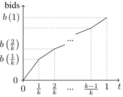
only at the points of the form mk, but it is continuous. See figure 3.
0
t
0
bids
1
k
2
k ... k−1
k 1
b 1k b 2
k b(1)
...
Figure 3: bidding function forf∈ Dk.
With the initial conditionb(0) = 0and the above differential equation being valid for the first interval 0,1
k
, we have uniqueness of the solution on this interval and, thus, a unique value ofb 1k
. Sincebis continuous, this value is the initial condition for the interval 1k,2
k
, where we again obtain a unique solution and the uniqueness of the valueb 2k
. Proceeding in this way, we find that there is a uniquebwhich can be a symmetric increasing equilibrium for an auction withf ∈ D∞. In sum, in the
supplement to this paper we prove the following:
Theorem 7 Assume thatuis twice continuously differentiable,u′ >0,f ∈ Dk,f is
symmetric and positive (f > 0). Ifb : [0,1]→Ris a symmetric increasing
equilib-rium, thenbis continuous in(0,1)and is differentiable almost everywhere in(0,1)(it is may be non-differentiable only in the pointsmk, form= 1, ..., k). Moreover,bis the unique symmetric increasing equilibrium. Ifu(x) =x1−c, forc∈[0,1),bis given by
b(x) =x−
Z x
0 exp
− 1
1−c Z x
α
f(s|s)
F(s|s)ds
Having established the uniqueness of the candidate for equilibrium, our task re-duces to verify whether this candidate is, indeed, an equilibrium. We complete this task in the next subsection.
Even if the reader insists on considering the more general set of p.d.f.’sD— being aware that this is a matter of mathematical generality, but not of economic generality — our setD∞is still dense inDand, thus, may arbitrarily approximate any conceivable
p.d.f. inD. In fact, the following result shows that equilibrium existence in the setD∞
is sufficient for equilibrium existence inD. This provides an additional justification of the method.
Proposition 8 Letf ∈ Dbe continuous and symmetric. IfTk(f)has a differentiable
symmetric pure strategy equilibrium for allk ≥k0, then so doesf, and it is the limit of the equilibria ofTk(f)askgoes to infinity.14
4.3
Equilibrium existence results
In the previous subsection, we established the uniqueness of the candidate for symmet-ric increasing equilibrium forf ∈ D∞. Letb(·), given by (3) withc= 0, denote such
candidate. LetΠ (y, b(x)) = (y−b(x))F(x|y)be the interim payoff of a player with typeywho bids as typex, when the opponent followsb(·). Let∆ (x, y) repre-sentΠ (y, b(x))−Π (y, b(y)). It is easy to see thatb(·)is equilibrium if and only if
∆ (x, y)≤0for allxandy∈[0,1]2. Thus, the content of the next theorem is that it is possible to prove equilibrium existence by checking this condition only for a finite set of points:
Theorem 9 Letf ∈ D∞be symmetric and strictly positive. There exists a finite set P⊂[0,1]2(precisely characterized in the supplement to this paper) such thatfhas a PSE if and only if∆ (x, y)≤0for all(x, y)∈P.
It is useful to say that the theorem is not trivial, since∆ (x, y)is not monotonic in the squares mk−1,m
k
× p−k1,kp
. Indeed, the main part of the proof is the analy-sis of the non-monotonic function∆ (x, y)in the sets mk−1,mk
× p−k1,pk
and the determination of its maxima for each of these sets. It turns out that we need to check different number of points (between 1 and 5) for each of these squares.
Using Theorem 9, we can classify whether or not there is equilibrium, and, through numerical simulations, obtain the proportion of cases with pure strategy equilibrium. That is, for each trialf ∈ Dk, we test whether the auction with bidders’ types
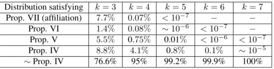
dis-tributed according to f has a symmetric increasing pure strategy equilibrium. The results are shown in the Table 2 below.
14See the definition ofTk
For eachk, 100%=distributions with equilibrium.
Distribution satisfying k= 3 k= 4 k= 5 k= 6 k= 7
Prop. VII (affiliation) 7.7% 0.07% <10−7 − −
Prop. VI 1.4% 0.08% ∼10−6 <10−7 −
Prop. V 5.5% 0.75% 0.01% <10−6 <10−7
Prop. IV 8.8% 4.1% 0.8% 0.1% ∼10−5 ∼Prop. IV 76.6% 95% 99.2% 99.9% 100%
Table 2 - Proportion off ∈ Dkwith PSE, satisfying properties IV-VII.
Table 2 shows that affiliation is restrictive even in the set of p.d.f.’s with symmetric increasing equilibrium. It is useful to record this fact separately. For this, let us in-troduce some useful notations. Letµandµkdenote the natural measures defined over
D∞ =∪∞
k=1Dk andDk, respectively, as constructed in the supplement to this paper
and letP andPk denote the set of p.d.f.’s inD∞andDk, respectively, which have a
symmetric increasing pure strategy equilibrium. From the above table, we extract the following observation:
Fact 10 Letµk ·|Pk
denote the measure induced byµkin the setDk∩ Pk. Then, we
haveµk A ∩ Dk|Pk
↓0.
Another way to say this is: there are many more cases with pure strategy equilib-rium than affiliation allows us to prove.
Unfortunately, however, the set of p.d.f.’s with symmetric increasing equilibrium is also small. This result is proved formally in the following:
Theorem 11 The measure of the set of densitiesf ∈ Dkwhich has PSE goes to zero
askincreases, that isµk Pk
↓ 0. Consequently, the measure of the set of densities
f ∈ D∞with PSE is zero, that is,µ(P) = 0.
Proof.See the supplement to this paper.
The proof of this theorem follows a simple idea: the equilibrium existence depends on a series of inequalities, the number of which increases withk. Although some care is needed for rigorously establishing the result, this simple observation is the heart of the argument.
The following table provides the numbers that come from numerical simulations and show that the convergence ofµk Pk
to zero is also very fast.
k= 3 k= 4 k= 5 k= 6 k= 7 k= 8 k= 9
With PSE 43.3% 22.2% 11.4% 5.6% 2.7% 1.3% 0.6% Without PSE 56.7% 77.8% 88.7% 94.4% 97.3% 98.7% 99.4%
The result summarized in Table 3 is negative in the sense that it suggests that the focus on symmetric increasing equilibrium may be too narrow. Nevertheless, this is not yet sufficient to conclude that most of the equilibria are in mixed strategies. In fact, while we know that mixed strategy equilibria always exist (Jackson and Swinkels 2005), there is the possibility — not considered in our results — that there are equilibria in asymmetric or non-monotonic pure strategies.
5
The Revenue Ranking of Auctions
This section is also divided in three parts. In the first subsection, we present negative results regarding the generalization of affiliation to other notions of positive depen-dence. In subsection 5.2 we propose a method for dealing with the problem of revenue ranking. In subsection 5.3 we describe the results obtained with the proposed method.
5.1
Generalization of affiliation’s revenue ranking
In this subsection we show that, for private values auctions, it is possible to generalize the existence for Property VI but not for Property V. Moreover, we provide an expres-sion for the difference in revenue from second and first price symmetric auctions that will be useful later.15 This is the content of the following:
Theorem 12 If f satisfies Property VI’ (see subsection 4.1), then the second price auction gives greater revenue than the first price auction. Specifically, the revenue difference is given by
Z 1
0
Z x
0
b′(y)
F(y|y)
f(y|y) −
F(y|x)
f(y|x)
f(y|x)dy·f(x)dx
whereb(·)is the first price equilibrium bidding function, or by
Z 1
0
Z x
0
Z y
0
L(α|y)dα
·
1−F(y|x)
f(y|x) ·
f(y|y)
F(y|y)
·f(y|x)dy·f(x)dx, (4)
whereL(α|t) = exph−Rt α
f(s|s)
F(s|s)ds
i
. Moreover, Property V is not sufficient for this
revenue rank.
Proof.See the appendix.
From the expression of expected revenue difference provided by Theorem 12, we see that the revenue superiority of the English (second price) auction over the first price auction seems to be strongly dependent on the condition required for Property VI′(see subsection 4.1). Moreover, the revenue rank is not valid even for a positive dependence concept as strong as Property V.
15The expression is not particularly difficult to obtain, but we were not able to find a reference for it.
5.2
How to solve the problem of revenue ranking?
In his interesting article about design economics, Roth (2002) compares the relation between economic theory and market design to the relation between physics and en-gineering and between biology and medicine and surgery. For instance, while physics offers simple and elegant models with clear indications, the actual problems in engi-neering require dealing with details that are not (and shall not be) considered in the basic physical model. But, as long as the specific environment is sufficiently deter-mined, engineers can detail the basic model to reach more precise conclusions.
Roth (2002)’s analogy suggests an answer to the question in the title of this sub-section. Basically, we need a two-level answer. In the first (theoretical) level with-out specific information, we need a clear prediction, obtained with a simple and basic model. Then, in the applied level, we need a methodology that allows the use of more detailed information (available in the specific case considered), to reach more precise conclusions.
We describe these two levels of the methodology in the sequel.
5.2.1 The basic model, without specific information
Not only the results in subsection 5.1, but also many results in auction theory (e.g. Maskin and Riley 1984, 2000), suggest that it is not possible to give simple predictions about the revenue ranking of auctions. The reason is that the expected difference of revenues can have any sign and the description of the set of distributions which has one or other sign is very difficult.
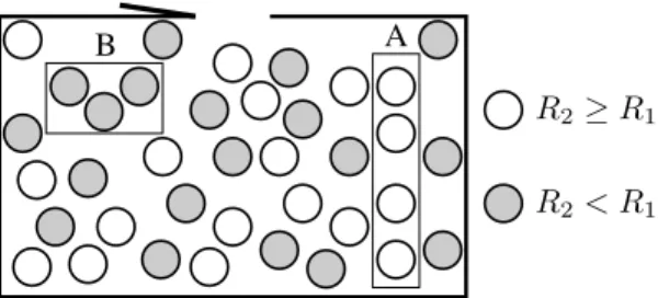
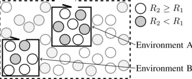
Fortunately, a simple characterization is available without further assumptions — if we work in the correct level of abstraction. To describe what we mean by “correct level of abstraction”, consider the following figure.
R2≥R1
R2< R1
B A
Figure 4: illustrative representation of the set of distributions with any kind of depen-dence.
The standard approach to the problem of revenue ranking of auctions is to give conditions (the sets A and B above) under which the revenue ranking is defined. Such approach is illustrated by Milgrom and Weber (1982)’s affiliation assumption and by Maskin and Riley (2000)’s three different assumptions for asymmetrical independent distributions.16 Under each of the these assumptions, the authors are able to say
pre-16The reader should not be confused with the citation of Maskin and Riley (2000), which do not treat
cisely what is the revenue ranking (the color of balls in the above figure). Now, if we think in the set of distributions as black box or an urn, and we want a “prevision” of the color of the ball that we are going to extract from it (the expected revenue ranking), the “correct” type of answer to our problem is the characterization of theprobabilityof obtaining one ranking or another.
Since we have the expression of the expected revenue difference, given by (4), we can obtain∆fR=Rf2−Rf1andr=Rf2−R
f
1
Rf2
, for eachf. Generating a uniform sample off ∈ Dk, we can obtain the probabilistic distribution of∆f
Ror ofr. The procedure
to generatef ∈ Dkis described in the supplement to this paper. The results are shown
in subsection 5.3 below.
Moreover, we can also obtain theoretical results about what happens for DN for
a largeN and even forD∞ =∪∞
k=1Dk. Nevertheless, for the last case, one has to
be careful with the meaning of the “uniform” distribution. In the supplement to this paper we show that a natural measure can be defined forD∞, which is analogous to
Lebesgue measure, although it cannot have all the properties of the finite dimensional Lebesgue measure.
As such, this context-free approach, without specific information, allows one to obtain theoretical results and previsions based on simulations. One possible objection to this approach is that it considers too equally the p.d.f.’s in the setsDk. But this is
exactly what we mean by “context-free”. If one has information on the environment where the auction runs, so that one can restrict the set of suitable p.d.f.’s, then this context-free approach should be substituted by the applied approach which we discuss next.
5.2.2 The applied approach, with specific information
Econometricians working in a specific auction environment may be able to restrict or characterize the set of distributions (dependence) that one finds in such environment.
R2≥R1
R2< R1
Environment A
Environment B
Figure 5: In specific auction environments — e.g. auctions of energy contracts, art ob-jects, timber, etc. — we mayexperimentallyfind different sets of typical distributions.
If we have the characterization of the typical distributions in an auction environ-ment, we may use the model presented in this paper and make simulations. In this fashion, we will be able to obtain more precise, context-specific indications about the revenue ranking of auctions in such environments.
difference between the two. With the standard approach, econometricians need to begin the analysis believing that the data obey such or such assumption.17 In our method, no assumption is required on the dependence of information. The restriction that one finds (and are illustrated in figure 5) comes from the data, not from theoretical restrictions. Methodologically, this is a big difference.
5.3
Results on Revenue Ranking
In the supplement to this paper, we develop the expression of the revenue differences from the second price auction to the first price auction forf ∈ Dk. Let us denote byRf
2
the expected revenue (with respect tof ∈ Dk) of the second price auction. Similarly, Rf1 denotes the expected revenue (with respect tof ∈ Dk) of the first price auction.
When there is no need to emphasize the p.d.f. f ∈ Dk, we writeR
1andR2instead
ofRf1 andRf2. Below, µandµk refers to the natural measure defined overD∞ =
∪∞
k=1DkandDk, respectively, as further explained in the supplement to this paper.
Fact 13 Eµk h
Rf2−R
f
1|f ∈ Dk
i
≈Eµk+1
h Rf2−R
f
1|f ∈ Dk+1
i
Fact 14 Eµk hRf
2−R
f
1
Rf2
|f ∈ Dki≈Eµ k+1
hRf
2−R
f
1
Rf2
|f ∈ Dk+1i.
The above enunciation is quite imprecise, because it does not give bounds for the approximation. This precludes us from calling them “theorems”. Nevertheless, there are mathematical arguments establishing them (in a more complex format, not worth discussing here). That is, the above “facts” are not only observations from the data. The interested reader is invited to see the details in the supplement to this paper. The same comments are valid for the following:
Fact 15 Eµ[R2−R1]&0.
We can make simulations to illustrate numerically the above results. We generated the distributionsf ∈ Dkas described in the supplement to this paper. (It is the same
process used in subsection 3.5 and section 4). We evaluate the revenue difference percentage, given by:
r= R
f
2−R
f
1
Rf2 ·100%,
that is, we carried out the following:
Numerical experiments
In what follows, we will treat the numerical simulations as giving an “experimental distribution” ofr. No confusion should arise between the “experimental distribution” ofrand the distributions generated by eachf ∈ Dk. We generated107distributions
f ∈ Dk, for k = 3, ...,9 and obtained r for each of such f. The “experimental
distribution” ofris characterized by the table below. It is worth saying that the results are already stable for 106trials.
Distribution: k= 3 k= 4 k= 5 k= 6 k= 7 k= 8 k= 9
Expectation 4.5% 8.0% 10.3% 12.1% 13.4% 14.6% 15.5%
Variance 5.3% 6.9% 7.3% 7.2% 7.0% 6.8% 6.6%
5% quantile −4% −3% −2% 0% 1% 3% 4%
10% quantile −2% −1% 0% 2% 3% 4% 6%
25% quantile 0% 2% 4% 6% 6% 8% 8%
50% quantile 2% 6% 8% 10% 10% 12.5% 12.5%
75% quantile 6% 10% 12.5% 15% 15% 17.5% 17.5%
90% quantile 10% 15% 17.5% 17.5% 19% 19% 19%
96% quantile 12.5% 17.5% 20% 20% 20% 20% 20%
99% quantile 15% 20% 25% 25% 25% 25% 25%
Table 4 - Expectation of the relative revenue differences (r) forf ∈ Dkwith PSE.
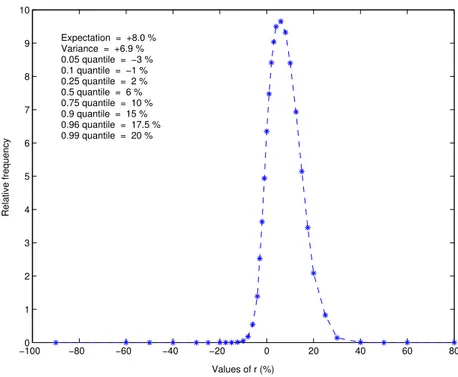
Figure 5 shows the “experimental density” (histogram) ofrfork= 4.
−1000 −80 −60 −40 −20 0 20 40 60 80 1
2 3 4 5 6 7 8 9 10
Values of r (%)
Relative frequency
Expectation = +8.0 % Variance = +6.9 % 0.05 quantile = −3 % 0.1 quantile = −1 % 0.25 quantile = 2 % 0.5 quantile = 6 % 0.75 quantile = 10 % 0.9 quantile = 15 % 0.96 quantile = 17.5 % 0.99 quantile = 20 %
Figure 5: Histogram ofrfork= 4, c= 0— for thosef ∈ Dkwith PSE.
Distribution k= 3 k= 4 k= 5 k= 6 k= 7 k= 8 k= 9
Expectation −0.08% 0.13% 0.28% 0.38% 0.46% 0.53% 0.57
Variance 10.5% 10.9% 10.5% 9.9% 9.4% 9.0% 8.5%
5% quantile −25% −20% −20% −17.5% −17.5% −15% −15%
10% quantile −15% −15% −15% −15% −12.5% −12.5% −12.5%
25% quantile −8% −8% −8% −8% −8% −8% −8%
50% quantile −1% −1% −1% −1% −1% −1% −1%
75% quantile 4% 6% 6% 6% 4% 4% 4%
90% quantile 10% 12.5% 12.5% 10% 10% 10% 10%
96% quantile 15% 15% 15% 15% 15% 15% 12.5%
99% quantile 25% 25% 25% 25% 25% 25% 25%
Table 5 - Expectation of the relative revenue differences (r) for all cases (with and without PSE).
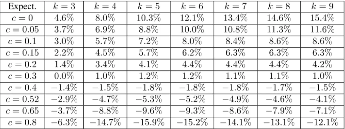
The following table allows one to compare the effects of dependence and risk aver-sion to the expected revenue differences. For this, we restrict to the case of CRRA bidders, that is, bidders with utility functionu(x) =x1−c, wherec∈[0,1).18
Expect. k= 3 k= 4 k= 5 k= 6 k= 7 k= 8 k= 9
c= 0 4.6% 8.0% 10.3% 12.1% 13.4% 14.6% 15.4%
c= 0.05 3.7% 6.9% 8.8% 10.0% 10.8% 11.3% 11.6%
c= 0.1 3.0% 5.7% 7.2% 8.0% 8.4% 8.6% 8.6%
c= 0.15 2.2% 4.5% 5.7% 6.2% 6.3% 6.3% 6.3%
c= 0.2 1.4% 3.4% 4.1% 4.4% 4.4% 4.4% 4.2%
c= 0.3 0.0% 1.0% 1.2% 1.2% 1.1% 1.1% 1.0%
c= 0.4 −1.4% −1.5% −1.8% −1.8% −1.8% −1.7% −1.5%
c= 0.52 −2.9% −4.7% −5.3% −5.2% −4.9% −4.6% −4.1%
c= 0.65 −3.7% −8.8% −9.6% −9.3% −8.6% −7.9% −7.1%
c= 0.8 −6.3% −14.7% −15.9% −15.2% −14.1% −13.1% −12.1%
Table 6 - Expectation of the relative revenue differences (r), for bidders with CRRA functionu(x) =x1−c, wherec∈[0,1).
6
Related literature, the contribution and future works
A few papers have pointed out restrictions or limitations to the implications of affil-iation. Perry and Reny (1999) presented an example of a multi-unit auction where the linkage principle fails and the revenue ranking is reversed, even under affiliation. Thus, their criticism seems to be restricted to the generalization of the consequences
18In Table 6, we restrict to the cases where PSE exists forc= 0. We do not have a generalization of the
PSE existence result (Theorem 9) — and, thus, we do not have a procedure to test for PSE existence — for
of affiliation to multi-unit auctions. In contrast, we considered single-unit auctions and non-affiliated distributions.
Klemperer (2003) argues that, in real auctions, affiliation is not as important as asymmetry and collusion. He illustrates his arguments with examples of the 3G auc-tions conducted in Europe in 2000-2001.
Nevertheless, much more was written in accordance with the conclusions of affil-iation. McMillan (1994, p.152) says that the auction theorists working as consultants to the FCC in spectrum auctions, advocated the adoption of an open auction using the linkage principle (Milgrom and Weber 1982a) as an argument: “Theory says, then, that the government can increase its revenue by publicizing any available information that affects the licensee’s assessed value”. The disadvantages of the open format in the presence of risk aversion and collusion were judged “to be outweighed by the bidders’ ability to learn from other bids in the auction” (p. 152). Milgrom (1989, p. 13) empha-sizes affiliation as the explanation of the predominance of the English auction over the first price auction.
This paper presents evidence that affiliation is a restrictive assumption. After devel-oping an approach to test the existence of symmetric increasing pure strategy equilib-rium (PSE) for simple density functions, we are able to verify that many cases with PSE do not satisfy affiliation. Also, the superiority of the English auction is not maintained even for distributions satisfying strong requirements of positive dependence. Neverthe-less, we show that the original conclusion of Milgrom and Weber (1982a) (that positive dependence implies that English auctions gives higher revenue than first price auction) is true for a much bigger set of cases , but in a weaker sense — “on average”.
We would like to highlight also two conceptual contributions of this paper that may go beyond the actual applications made here.
One of these is the restriction to a simple space of distributions. The proposed space makes possible the complete characterization of the symmetric increasing pure strategy equilibrium existence problem, because it requires only elementary (although lengthy) calculations. The set of distributions considered is as general as need for economic applications and seems suitable for modeling the asymmetric bidders case as well.
The second conceptual contribution is the way of looking at the problem of revenue ranking. We propose two levels of the answer: an abstract, theoretical level and a simulation-driven applied level.
The first level allows general theoretical conclusions that may be useful as general, context-free guidance. Using the second level, applied economists can reach case-specific conclusions which may be more accurate and valuable.
These ideas are applicable for more general setups than those pursued here. Not only equilibrium existence but also the revenue ranking can be investigated in con-texts ofnasymmetric bidders, interdependent values, risk aversion and multi-units. Although these generalizations seem doable, they are by no means trivial.19
Nevertheless, the main complement to this work seems to pertain to the fields of
19The generalization fromn = 2to generalncan be pursued, at least for the symmetric case, using
the expressions developed in the supplement of this paper. Only, instead of considering the expressions of
f(x|y)andF(x|y)as coming from a bivariate distribution, we could write the expressions as coming from
econometrics and experimentation. This is to develop a method to characterize the de-pendence (sets of distributions) typical in each specific situation. With such a method, applied works could characterize what happens in specific auctions. For instance, it is likely that the kind of dependence that appears in mineral rights auctions, or in elec-tricity market auctions, is distinct from that observed in art auctions.
If such a method is developed and if the correspondent specific characterizations are done — these are big if’s — we could find a way to explain why some kinds of markets almost always use a specific auction format, as observed by Maskin and Riley (2000): “rarely is any given kind of commodity sold through more than one sort of auction. Thus, for example, art is nearly always auctioned off according to the English rules, whereas job contracts are normally awarded through sealed bids” (p. 413). Maskin and Riley (2000) comment that the Revenue Equivalence Theorem is not able to explain such case-specific uniformity. The same argument also applies to affiliation, which would predict the use of English auction for every situation.
An auction theory model capable of general conclusions and context-specific cali-brations, using simulations and theoretical analysis, could explain this. If not, at least it will be more realistic and, thus, more useful.
Appendix
Proof of Theorem 1.
It is obvious that(III)⇒ (II) ⇒(I). The implication(IV)⇒ (III)is Theorem 4.3. of Esary, Proschan and Walkup (1967). The implication(V)⇒(IV)is proved by Tong (1980), chap. 5, p. 80. Thus, we have only to prove that(V I)⇒(V), since the implication(V II)⇒(V I)is Lemma 1 of Milgrom and Weber (1982a). Assume that
H(y|x) ≡ Ff((yy||xx)) is non-decreasing inxfor ally. Then,H(y|x) = ∂y[lnF(y|x)]
and we have
1−ln [F(y|x)] =
Z ∞
y
H(s|x)ds>
Z ∞
y
H(s|x′)ds= 1−ln [F(y|x′)],
if x > x′. Then, ln [F(y|x)] 6 ln [F(y|x′)], which implies thatF(y|x) is
non-increasing inxfor ally, as required by propertyV.
The counterexamples for each passage are given by Tong (1980), chap. 5, except those involving property (VI):(V) ; (V I),(V I) ; (V II). For the first counter
example, consider the following symmetric and continuous p.d.f. defined on[0,1]2:
f(x, y) = c 1 + 4 (y−x)2
f(y) = k
2[arctan 2 (1−y) + arctan 2 (y)]
so that we have, for(x, y)∈[0,1]2:
f(x|y) = 2h1 + 4 (y−x)2i−1[arctan 2 (1−y) + arctan 2 (y)]−1,
F(x|y) =[arctan 2 (x−y) + arctan 2 (y)] arctan 2 (1−y) + arctan 2 (y)
and
F(x|y)
f(x|y) = 2
h
1 + 4 (y−x)2i[arctan (2x−2y) + arctan (2y)].
Observe that fory′= 0.91> y= 0.9andx= 0.1,
F(x|y′)
f(x|y′) = 0.366863>0.366686 =
F(x|y)
f(x|y),
which violates property (VI). On the other hand,
∂y[F(x|y)] =
2 1+4y2 −
2 1+4(x−y)2
arctan (2−2y) + arctan (2y)
−[arctan (2x−2y) + arctan (2y)]
h
2 1+4y2 −
2 1+4(1−y)2
i
[arctan (2−2y) + arctan (2y)]2
In the considered range, the above expression is non-positive, so that property (V) is satisfied. Then,(V);(V I).
Now, fix anε <1/2and consider the symmetric density function over[0,1]2:
f(x, y) =
k1, ifx+y62−ε
k2, otherwise
wherek1>1> k2 = 21−k1 1−ε2/2/ε2>0andε∈(0,1/2).For instance,
we could chooseε = 1/3, k1 = 19/18 andk2 = 1/18. The conditional density
function is given by
f(y|x) =
1, ifx61−ε
k1
k2(x+ε−1)+k1(2−ε−x), ifx >1−εand ify62−ε−x
k2
k2(x+ε−1)+k1(2−ε−x), otherwise
and the conditional c.d.f. is given by:
F(y|x) =
1, ifx61−ε
k1y
k2(x+ε−1)+k1(2−ε−x), ifx >1−εand ify62−ε−x
k2(y+x+ε−2)+k1(2−ε−x)