COMPARATIVE ACCURACY EVALUATION OF FINE-SCALE GLOBAL AND LOCAL
DIGITAL SURFACE MODELS: THE TSHWANE CASE STUDY I
A. Breytenbach
Council for Scientific and Industrial Research, Pretoria, South Africa - [email protected]
KEY WORDS: 3D,DSM, DTM, InSAR, LiDAR, Topography, Tri-Stereo, WorldDEM
ABSTRACT:
Conducted in the City of Tshwane, South Africa, this study set about to test the accuracy of DSMs derived from different remotely sensed data locally. VHR digital mapping camera stereo-pairs, tri-stereo imagery collected by a Pléiades satellite and data detected from the Tandem-X InSAR satellite configuration were fundamental in the construction of seamless DSM products at different postings, namely 2 m, 4 m and 12 m. The three DSMs were sampled against independent control points originating from validated airborne LiDAR data. The reference surfaces were derived from the same dense point cloud at grid resolutions corresponding to those of the samples. The absolute and relative positional accuracies were computed using well-known DEM error metrics and accuracy statistics. Overall vertical accuracies were also assessed and compared across seven slope classes and nine primary land cover classes. Although all three DSMs displayed significantly more vertical errors where solid waterbodies, dense natural and/or alien woody vegetation and, in a lesser degree, urban residential areas with significant canopy cover were encountered, all three surpassed their expected positional accuracies overall.
1. INTRODUCTION
The digital representation of the Earth’s topographic surface as a regular grid amplified with diverse vegetation, manmade features and bare terrain seamlessly manifested as elevation values have become commonplace in the modern digital era. Where sufficient bandwidth and connectivity exist today, even the layman can experience 2½D or 3D data representations at home or office via popular web viewers or applications. Enabled by remote sensing (RS) technology used in Earth Observation in particular, one can appreciate and visualise familiarities in the approximated landscapes, in most cases even right up to your own neighbourhood or doorstep. This feat is technically supported and enhanced thus far by a DEM, nowadays covering the entire Earth and can be of truly remarkable quality. When the user base extends further to the more meticulous aeronautic, engineering, military and mining fields, for example, an even higher expectation and emphasis is placed on the reported positional accuracy and precision of said elevation surface (Reuter and Kersebaum, 2009).
1.1 Generating and Modelling Topographic Data
Mankind have over the last two decades successfully managed to collect vast amounts of suitable digital information to model and represent topographic surfaces. Other than traditional land surveying methods, the geo-information was largely collected by dedicated aerial and space missions. Observing from a known location and attitude, it can be passive optic sensors detecting a vast array of reflective measurements from Earth or return signals recorded from an active sensor. DEMs constructed from topographic images have a specific support size (a fixed area or volume of the land surface that is being sampled) that equals the original scanning resolution (Hengl and Evans, 2009). The values recorded at cell nodes thus represent the average value of all possible elevations in those pixels. Conversely, an active laser sensor would have a relatively small support size (in mm). Innovative DEM
extraction methods, interpolation and even fusion techniques routinely produce accurate point clouds or an elevation grid (Nelson et al., 2009) to compose a seamless topographic surface. Used to correspond to terrain relief, a DEM is a digital representation of continuous elevation values over a topographic surface by a regular array of x, y, and z values, all referenced to a common datum. As illustrated in Figure 1, the edited first stage DSM represents a continuous land surface that includes the elevation or orthometric height (in meters) of projected off-terrain objects such as buildings and vegetation, locally referenced to mean sea level (MSL). The reference geoid represents the equipotential surface of Earth’s gravity field that coincides on average with MSL (Chandler and Merry, 2010). The DSM can be converted further to a digital terrain model (DTM) – a digital representation of variables relating to the Earth’s topographic surface. The DTM is still referenced to MSL, but now technically devoid of any man-made features and vegetation after being subjected to some extensive editing and interpolation processes. The main production challenges faced here normally are to preserve the scale characteristics of different DEM (Poli et al., 2009) whilst preserving terrain continuity (Doytsher et al., 2009).
Figure 1. Seamless manifestations of various DEM types as constructed from directly measured or extracted geo-referenced
height observations from the air or from space ISPRS Annals of the Photogrammetry, Remote Sensing and Spatial Information Sciences, Volume IV-2/W1, 2016
When successful, the normalised DEM (or nDEM) can then be generated by simply computing the difference between the DSM and DTM grids (Fig.1; bottom-right). Essentially an elementary height model now, the nDEM values would normally range from zero meters at ground level (the DTM) to the vertical height of the tallest feature or point (contained in the DSM). If the DEM ground sampling distance (GSD) equates to exactly one meter, each cell value would theoretically also represent the precise volume (m3) of that pixel in 3D space, as
referenced from the Earth’s ‘bare’ surface (Grohmann et al., 2011). By definition though, since only a single elevation value can be stored per grid cell, this dimension will only resonate true for solid materials or city fabrics at a particular scale; much less so where storied vegetation, tunnels, overhangs and typical occlusions occur in urban landscapes.
1.2 Study Rationale
In South Africa progress was made from the previous 200 m and 50 m GSD national DEMs to the present version made available by the State’s custodian – grid nodes available at 25 m postings. Essentially a DTM, it unfortunately still only covers roughly two-thirds of the country at present and will only be completed sometime in future. Therefore, along with the global geospatial community elsewhere facing similar 3D data needs (Milevski et al., 2013; Rexer and Hirt, 2014), GIS practitioners, professionals and scientists in South Africa have rapidly acquainted themselves with alternative DEM sources, particularly with the 1 arc-second (~30 m) Shuttle Radar Topography Mission (SRTM) DEM product. Before the worldwide release of this original base dataset was announced by the US Government in September 2014, the need for and considerable dependency on this aging dataset collected in February 2000 was previously met by the degraded 3 arc-second product (Van Niekerk, 2015), subsequent official and unofficial versions thereof or alternatively the research-grade ASTER GDEM 1 arc-second version released in 2009 (Hirt et al., 2010; Hengl and Reuter, 2011; Pulighe and Fava, 2013). Under the currently proposed National DEM System (NDEMS) program, preliminary expert investigations into the feasibility of producing a new fine-scale seamless DEM for South Africa in a sustainable and cost-effective manner have commenced. With other DEM products also available commercially, this study formed part of the larger technical research component that focused on the accuracy evaluation of suitable off the shelf DEM alternatives in relation to those that can be produced cost-effectively from existing national ortho-optic data sources. The paper will deal specifically with the accuracy evaluation and results of the sampled DSM products.
2. STUDY AREA, DATA AND METHODS
2.1 Study Region
The area of interest identified for conducting the study stretches from the Pretoria central business district eastwards towards the Mamelodi Township; all located within the greater City of Tshwane metropolitan area. The 348 km2 region of interest was chosen to perform the comparative DSM accuracy tests primarily because it is characterised by diverse topography and land cover. The topography ranges from mountainous areas of the Magaliesberg Mountain range that often contain natural ecosystems, to relative flat plateaus covered by a variety of urban settlement patterns and activities that typifies a flourishing capital city in South Africa.
2.2 Data Selection and Preparation
Three gridded height surfaces were considered as the primary input in this positional DSM accuracy evaluation, namely:
i. an experimental 2 m GSD base DSM constructed from digital aerial photography through stereo-pair matching; ii. a 4 m GSD Elevation4™ DSM product generated from tri
-stereo image acquisitions from an operational Pléiades satellite; and
iii. the 0.4 arc-second WorldDEM™ DSM global product created from radar data collected by the ongoing TerraSAR-X add-on for Digital Elevation Measurements (TanDEM-TerraSAR-X) mission using StripMap beam mode in X-band frequency.
The reference height grids – all with 32-bit precision and at corresponding spatial resolutions – were constructed from concisely measured geo-referenced lidar data. It was collected by an airborne survey conducted over the study region between Sep. and Oct. 2013 (spring season). A random selection of this point cloud was also used as independent control points (ICPs). For comparative reasons and considering the radar acquisitions occurred (mainly) between 2011 and 2013, the time difference between all the selected height datasets did not exceed two years. The aerial photography campaign was flown in May 2012 during the autumn season, whilst the tri-stereo collection was completed just two weeks before the lidar survey. The need to assess positional DEM accuracy separately within topographically diverse classes across the entire surface was facilitated with two ancillary datasets. The nominal inputs included a recently published National Land-Cover raster dataset as well as derived surface gradient layers. Acquired simultaneously with the aforementioned lidar mission was optical data captured with a Kodak KAI-11002 dual charge coupled device (CCD) to later produce digital RGB aerial ortho-photos (10 cm GSD). A waterbody layer (shapefile) digitised from the above imagery too provided the exact extents of any significant water surface that appeared in 2013 across the region. The next four sub-sections will provide more technical details regarding the origin (sensor) and creation of each of these gridded elevation surfaces and their characteristics, together with those of the ICPs and reference datasets used during the accuracy evaluation process.
2.2.1 Aerial Photography with Stereo Pairing:
The feasibility of utilising spatial data obtainable from the State’s custodian as primary input for DEM production remained at the forefront of investigations in South Africa at time of writing. In this instance photographs (normally) captured with a Digital Mapping Camera at 50 cm GSD, along with the recorded location (latitude, longitude and altitude) and attitude (roll pitch and heading) of the aircraft in motion, were essential. As prescribed by the National Standard for the Acquisition of Digital Aerial Imagery, the horizontal positional accuracy of the pixels constituting this imagery shall not exceed three metres at the 95% confidence level (CD:NGI, 2010). Consequently the base DSM generated and sampled for this study was deemed the best performing prototype when the initial research emphasis was placed on determining the least number of bands and optimal stack depth the elevation model needs, but which is essential for seamless, but reliable baseline DEM construction. The necessary data, including the camera calibration and triangulation information, was obtained from the Chief Directorate: National Geospatial Information (CD:NGI). The data over the region of interest was collected on the 26-27th ISPRS Annals of the Photogrammetry, Remote Sensing and Spatial Information Sciences, Volume IV-2/W1, 2016
of May 2012 between 11:00 and 13:30. Each (flight) strip consists of images with a standard forward overlap of between 55% and 65% and a lateral overlap of between 25% and 40%. The flying altitudes ranged between 6,200 m to 6,500 m with the viewing geometry set about nadir and the focal length at 120 mm. The resulting stereo coverage then allows for the automated extraction and generation of height data as overlapping gridded DEM segments.
The toolsets and algorithms used to collect adequate ground control points (GCPs), establish epipolar geometries and extract the raw orthometric heights were all available in PCI Geomatica™ software, OrthoEngine in particular. It can be programmed to speedily process a quality DEM where the camera distances for each pair of pixels in overlapping aerial photographs are available (PCI Geomatics, 2013). The camera calibration data were used to set up the camera model, while the triangulation data was used to set up the exterior orientation of the raw (unrectified) aerial photographs. The camera's recorded position variables were used to calculate surface elevation using sound photogrammetric principles and finally compute qualified cells as height above a reference geoid in the specified georeferenced framework. For the DSM prototype, only the panchromatic green band was used during the epipolar DEM extraction process. A total of 33 overlapping gridded DEM segments over the surveyed area were generated. Additional DEM editing and enhancements processing chains were developed with ESRI ArcGIS 10.x software and these customised workflow modules executed with the extracted, unedited DSM as the primary input. Semi-automated routines included running a Gaussian 15x15 filter and generating a first Principal Component from the associated RGB bands for auxiliary cell values. These were useful during the ensuing DSM segment by segment merging process and to eliminate random pixels regarded as extreme outliers (based on standard deviation). These values are usually responsible for the typical ‘pit’ artefacts found in a DEM. Although the region of interest is predominantly urban and built-up in nature, some of the last-mentioned routines were of course essentially designed to cater for national coverage production, here particularly to improve the 3D construction of relatively large productive agricultural fields, including woody plantations. This is because considerably large voids in the DEM are often uncovered here locally for a variety of reasons, e.g. due to waterlogging, glare, vegetation structure or excessive shadows. The final GIS routines filled any remaining voids systematically. Cells nominally representing significant water bodies in the raster or certain wide transport features were finally artificially flattened to ultimately produce the seamless DSM prototype at 2 m postings that was included in this study.
2.2.2 VHR Satellite Imagery with Tri-stereo Coverage:
Phased 180° apart, the Pléiades-1A&B satellite constellation follows a near-polar sun-synchronous orbit around the Earth in order to deliver ortho-optic products. The in-track agility of modern high-resolution satellite image (HRSI) systems is as advantageous when attempting to map dense vegetation types or forests as when representing heterogeneous 3D city landscapes with high-rises, large complex buildings and informality abound (Krauss and Reinartz, 2010). Just past 10 am on September 8 2013, the Pléiades-1B satellite collected what was virtually cloud-free tri-stereo imagery over the study region. Pléiades images (panchromatic) are acquired with a 70 cm GSD at nadir. Orbiting along at 7.5 km/s at an altitude of 694 km, the data was collected with about 22 second lapses between the consecutive
acquisitions. Set at a focal length of 12.905m, the single alongtrack viewing angles alternated from 12.554° to 1.939° to -12.128°, whereas the across-track viewing angles was curbed at -1.114° on average. Yet, unlike the aerial frame cameras, the HRSI systems in question are based on the push-broom scanner model, with its CCD arrays used for panchromatic detection in Time Delay Integration mode (Coeurdevey and Gabriel-Robez, 2012). It remains challenging to establish epipolar geometry with this sensor model in space despite the resampling methods abound (Oh, 2011), such as the Rational Polynomial Coefficients method – a sensor model distributed by most of the commercial operating satellites. The downloaded data was therefore processed internally by the supplier using a customised industrial and multi-sensor automated processing chain implemented for bulk ortho-optic and 3D production. The automatic stereo matching processing, including a global auto-filtering of artefacts, are performed by the system, and is followed by additional manual editions. These are primed towards hydrological enhancements, the removal of spurious artefacts (spikes, voids) and the cleaning or removal of artificial obstructions observed in urban main roads. After completing the editing tasks, any remaining void is then interpolated to deliver the final digital elevation surface according to the set standards and (verified) product specifications, namely a 32-bit precision Elevation4™ DSM.
2.2.3 Space Borne SAR Interferometry:
The TanDEM-X mission is currently realized as the trendsetter in global DEM production when operating the phased radar instruments as a single-pass SAR interferometer (InSAR). Oversaw in the framework of a Public Private Partnership between the German Aerospace Center and Airbus Defence and Space, the primary objective of the TanDEM-X mission is the construction of a high quality, consistent (seamless) global DEM as the basis for a wide range of scientific research, as well as for operational and commercial DEM generation (Airbus DS, 2014). To accomplish the mission’s unique goals, the TerraSAR-X/ TanDEM-X satellites operate as a single-pass InSAR, typically in the bi-static StripMap mode. The instruments on the TerraSAR-X satellites are advanced X-band SAR based on active phased array technology which can be operated in different imaging modes and with multi-polarization capability (Krieger et al., 2010). Furthermore, and in contrast to the passive sensors described earlier, the modern SAR systems on board not only acquire data reliably since they operate independent of cloud coverage and lighting conditions, but the fine spatial resolution (up to 25 cm in staring SpotLight mode) with increased radiometric quality (and vegetation penetration) offers large potential benefits not only to those involved in geomorphometry, but also to a variety of other Earth Observation or space related research fields and industries (Hajnsek et al., 2014). Each spacecraft orbit the Earth in the phased Helix satellite formation, selected specifically for operational DEM generation (Krieger et al., 2013), since it enables an interferometric mapping of the complete Earth surface with a stable height of ambiguity using a small number of formation settings. The large initial along-track separation of 76 km (10 seconds) between the satellites also enables the observation of slow drifts and movements (Krieger et al., 2010). From the bulk of the SAR data collected in under three years, a homogeneous DEM covering the entire Earth’s land mass (150 Mkm²) was generated and made commercially available in 2014 as the WorldDEM™ product (Airbus DS, 2014). Producing the world’s first High Resolution Elevation (HRTE3) level DEM – formerly a Digital Elevation Terrain Data (DTED-3) product – ISPRS Annals of the Photogrammetry, Remote Sensing and Spatial Information Sciences, Volume IV-2/W1, 2016
was essentially achieved with two global single-pass InSAR collections and by using in-house customised interferometry and editing software. This seamless product is a refined DSM ensuring hydrological consistency, i.e. flattening of water bodies and consistent flow of rivers, and includes editing of shore- and coastlines. The grid spacing of the obtained DSM product was 0.4 arc seconds in latitude. It was a sample of this reportedly accurate global DSM product clipped over the region of interest that was made available for this technical evaluation.
2.2.4 Airborne Laser Scanning:
As the demand for very high resolution data from active sensors grow, many industries nowadays rely on specially designed laser-based systems for the acquisition of height and return signal intensity data (Al-Durgham et al., 2010). Operating active sensors that fall into the category of airborne instrumentation known as lidar (Light Detection And Ranging) have gained in popularity in those spheres of industries where highly detailed and accurate 3D data is essential for realizing their strategic planning, management, maintenance, service and other operational goals (ASPRS, 2013). Routinely mounted on a variety of airborne platforms, Airborne Laser Scanning (ALS) systems can capture highly accurate topographic data. By measuring the location and attitude of the cruising aircraft, the Euclidean distance to ground and scan angle (with respect to the base of the laser scanner housing), a precise 3D ground position for the impact point of each laser pulse can be determined. This yields direct, 3D measurements of the ground surface, vegetation, buildings and roads as required. The ability to digitize either the signal strength or the range to the reflecting surface is dependent on that surface having adequate reflectivity (Demir et al., 2009). However, provided each target results in adequate signal strength for detection, a lidar system is normally capable of detecting up to four targets for each outbound laser pulse (first, second, third, last). Tinkham et al. (2012) investigated how surface morphology and vegetation structure influence DEM errors. Vegetation structure was found to have no influence, whereas increased variability in the vertical error metrics was observed on steeper slopes (> 30°), thus illustrating that lidar classification algorithms are not limited by high-biomass forests, but rather that slope and sensor accuracy both play important roles.
Each check point and base reference DSM used in this investigation originated from ALS data. It was surveyed from a fixed wing aircraft flying at an altitude of around 1,500 m and covered the entire Tshwane metro. The campaign was divided into three flight blocks within which the flight line orientations of two (B & C), as intersected by the study region, differed. The ALS system used for the mission was equipped with a multiple-return intensity measurement feature that enabled one to measure the sizes of the reflected returns at various levels off e.g. roofs of buildings or a forest canopy (up to the first three returns; see top left in Fig. 1). This in addition to the distances to each reflecting surface as measured by the range counting cards. Operating the instrument, a Leica ALS50-II lidar sensor, at a scan angle of 37° and with a vertical discrimination distance of approximately 3.5 m for multiple targets (pulse rate of 145 KHz; scan frequency of 46.9 Hz), the region was completely surveyed. Following this, Global Positioning System (GPS) and inertial measurement units (IMU) processing software combined GPS base station data with IPAS airborne GPS data to provide a differential GPS aircraft position solution, where after this was combined with Scanner Assembly IMU data to provide smoothed position and orientation data. With
multi-pulse mode enabled and with the 30% strip overlap achieved, this resulted in (on average) eight observations per square meter on Earth. The return signal intensity data was processed into a dense point cloud and then ultimately classified into discreet ground and non-ground points using a single algorithm across the entire area of interest. These classified x,y,z measurements formed the primary input when generating both a seamless 32-bit DTM and DSM baseline product at two meter postings within a standardised georeferenced framework. This was achieved mainly by using the ANUDEM algorithm (Hutchinson et al., 2011) available in ArcGIS10.x as the ‘Topo to Raster’ tool (v5.3) to produce the base DTM, as well as running other DSM construction and quality enhancements routines when executing the customized DEM processing chains. The other reference DTMs and DSMs required to quantify the relative (or point-to-point) accuracy of each of the selected DSMs in matching spatial resolutions was created by resampling the above 2 m GSD base DEMs using a bilinear interpolation method and restricting the conversion factor between 2.0 and 2.5 in each instance. In the case of the Elevation4 DSM, reference DEMs were directly resampled to 4 m GSD, and in the case of the WorldDEM product, the 12 m GSD reference DEMs were created first by producing an intermediate 5 m elevation grid, which in turn was then resampled to the required 12 m GSD reference DEM. The recorded (absolute) positional accuracy of these respective (co-registered) resampled reference elevation grids was found to be comparable to that of the original 2 m GSD base DTM and DSM (≤ 1.0 m RMSEz).
2.3 Study Design
In order to locally quantify and compare DSM quality, the study design consisted of three basic tests: the first evaluating absolute vertical accuracy, the second relative vertical accuracy and the third relative horizontal accuracy. The three individual DSMs selected for this evaluation were measured against the ICPs and gridded reference DEMs. The resulting error measures were analysed in further detail across relevant topographic elements that included digital layers representing the dominant primary land cover/ land use (LCLU) classes of that period, as well as classified slope rasters that were calculated (% rise) from the corresponding reference DTMs. The release of the 2013 - 2014 South African National Land-Cover dataset by government for public consumption (GEOTERRAIMAGE, 2014) formed the official LCLU dataset of choice to include in this comparative DSM accuracy evaluation. Of the fifty-two tertiary classes (of a possible 72) present in the study area, these were regrouped into nine LCLU super-groups, namely i) Waterbody; ii) Wetland/ Grassland/ Golf; iii) Thicket/ Dense bush/ Woodlot; iv) Woodland/ Open bush; v) Cultivation; vi) Bare/Mines; vii) Urban Commercial/ Industrial; viii) Urban Residential (dense to open trees/bush); ix) Urban Residential (low veg/grass/bare). The surface gradient break values were 1.5, 2.0, 5.0, 10.0, 20.0 and 40.0 percent rise and greater. Any ICP could then, by performing a spatial join in GIS, be allocated a LCLU or slope attribute. The LCLU class at each check point was also validated by manual interpretation using the 10 cm RGB ortho-photos. During the relative accuracy evaluation process, this modified LCLU raster, originally distributed as a 1 arc-second product, was resampled to match the GSD of the DSM under review, using a nearest neighbour interpolator. This was done in order to extract and separately assess the error measures grouped within each LCLU class in more detail, but consistently according to scale given the original ~30 m support size.
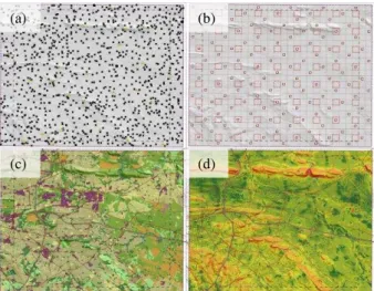
For absolute vertical accuracy calculations the superior1 lidar data functioned as the ICPs. The spatial distribution of check points or GCPs plays an important role in the accurate processing and evaluation of most ortho-optic data. When investigating the geometric quality of WorldView-2 image data, Da Costa’s (2010) preliminary results showed that the one -dimensional RMS error based on the manual measurement of a group of equally distributed ICPs is sensitive to the DEM accuracy. Further testing was recommended, especially for less accurate DEM data, diverse terrains and images characterised by high satellite inclination angle. The recommendation is to use as many points as possible and try to evenly space the points throughout the project area (ASPRS, 2013), but preferably not entirely systematic, evenly spaced control points. Thus a special algorithm was developed to harvest the appropriate number georeferenced elevation values from the available candidates in the lidar point cloud. It executed according to a stratified random selection process and robust proximity analysis that related directly to the underlying resampled LCLU or slope data. This was performed beforehand in order to closely and uniformly represent the aerial coverage each LCLU or slope class in proportion to all qualified cells, thus a pro rata number of random ICPs per class respectively. No ICPs were available within waterbodies when determining absolute accuracy. The final spatial distribution of the returned lidar data points across the entire study region is mapped in Figure 2(a), as well as some of the (b) systematic DEM sample patches used to produce displacement vectors. Also indicated are 25 existing trigonometric beacons which, together with the 1,422 ICPs selected, functioned as ground control points when the absolute accuracy of the Elevation4 and WorldDEM DSM products were determined. Of this total of available 1,447 ICPs, the experimental DSM used 1,118 of these, i.e.19 trig beacons and 1,099 ICPs.
Figure 2. The distribution of the (a) ICPs and (b) sample patches over the region of interest, as well as the (c) nine LCLU
types and (d) seven slope classes present
Also shown is (c) the LCLU classes and (d) slope classes in question. The slightly smaller extent of the DSM prototype (the
1 The required vertical accuracy for the ALS survey was set to 0.08 m
(RMSE) whilst premarks were utilized as GCP ground control. The Tshwane post-survey validation results, sampled across 30 points, revealed a mean vertical difference of +0.078 m and standard deviation of 0.059 m; with the obtained RMSEz measuring 0.062 m.
hashed rectangle) was constrained to the 276 km2 area surveyed by the aerial mission.
2.4 Assessing DSM Accuracy
The most common measure of DEM quality is absolute vertical accuracy, which theoretically accounts for all effects of systematic and random errors (Fisher and Tate, 2006). For some applications of DEMs however, the relative vertical accuracy (or geomorphological accuracy), which is controlled by the random errors in the dataset, is of much more importance than the absolute measure. Reuter et al. (2009) clearly indicated that the relative vertical accuracy of a gridded elevation surface is especially important for second- and third terrain derivatives (such as calculating slope, aspect and land forms), which make use of the local differences among adjacent elevation values. Thus the same statistical descriptors can be computed to evaluate the relative (point-to-point) accuracy of each sample DSM as measured against the reference data and matching the cell sizes. The vertical accuracy of the DSMs was sampled against the stratified randomly selected lidar measurements or ICPs (absolute error) and the prepared gridded reference surfaces (relative error). When extracting the height values from a sample DSM, a bi-linear interpolated value from the immediate 3x3 cells in the vicinity of the ICP was calculated. Vertical error in meters was calculated as:
reference
sample h
h
h
(1)
where ∆h = total vertical error distance hsample = sample DSM cell node height hreference = control point or reference height
The statistical measure of the magnitude of a varying quantity, here the difference between the sample and reference height value, was expressed by RMSEz (also known as the quadratic
mean). Particularly useful when variates have positive and negative signs (ASPRS, 2013), root mean square error was calculated as:
n
i i
z h
n RMSE
1 2 1
(2)
where RMSEz = root mean square error of sample n = number of ICPs or cell nodes (pixels)
The sample mean of all errors was calculated as:
n
i i
h n u
1 1
ˆ (3)
where û = mean error of sample
A common statistic used to express DEM error when variates are of both signs is mean absolute error (MAE). It is the arithmetic mean of the absolute error of the different height measurements in question. The formula used to calculate MAE was:
n h
MAE
i (4)(a) (b)
(c) (d)
where MAE = mean absolute error of sample
It is thus a statistic quantity used to measure how close forecasts or predictions are to the eventual outcomes (Fisher and Tate, 2006). Another useful descriptor of dispersion or variability less sensitive to outliers is the normalised mean absolute deviation (NMAD). A measure of central tendency particularly suitable for fine-scale DEMs (Höhle and Höhle, 2009), it is proportional to the median of the absolute differences between observed errors and the median error of the sample. In its general form, NMAD was calculated as:
) (
4826 .
1 median h m
NMAD i i h (5)
where NMAD = normalised median absolute deviation m∆h = median of the individual errors i = 1 …n
The sample’s standard deviation (STDDEV) is a similarly useful error statistic that indicates how tightly data are clustered around the population mean. Therefore a good measure of the reliability of the mean error value, STDDEV was calculated as:
n
i i
n h u
σ
1 ) 1 (
1
) ˆ
( (6)
where σ = standard deviation of sampled errors
There are straightforward conversion factors to translate among the three common error metrics of RMSEz, LE90, and LE95
(Maune et al., 2007). Vertical accuracy was calculated next expressed as LE90 by using the standard conversion factor:
z
z RMSE
Accuracy 1.6449 (7)
The final vertical accuracy statistic calculated was the 90% contour interval (90% CI) and, by again using the conversion factor applicable at that particular confidence level, was calculated as:
z
z RMSE
Accuracy 0.5958 (8)
These statistical accuracy descriptions represent the probability that a feature is within a given distance of its true location, here in the vertical dimension. The threshold for outliers (N) throughout the assessment was set at ±3.0σ and any error value beyond these two break-values was disregarded in the final error and accuracy computations. The reported vertical error (RMSEz of 0.062 m) of the Tshwane lidar survey was deemed
trivial enough to not add it to the overall user error.
Horizontal accuracy was tested by comparing the planimetric coordinates of well-defined points in the dataset with coordinates of the same points from an independent source of higher accuracy. When generally dealing with the positional accuracy of digital geospatial data, the probability that a feature is within a given radial distance of its true location is represented by RMSEr (ASPRS, 2013). This statistical
description, or probability, can also be represented as CE90 (circular error 90%), CE95, etc., where the other two descriptors would state the measurement and unit, e.g. 2.5 m CE90. In the case of DEMs however, calculating this planimetric statistic is not the elementary task it appears to be.
Although all efforts are usually made to preserve the scale characteristics of different DEMs at its specific GSD (Poli et al., 2009), it remains nearly impossible to have any of the check points placed at the very centre of any individual cell in the gridded DEM. Or, if a control point represents a physical feature or structure on Earth e.g. a trigonometric beacon, it will not necessarily be observable in the DSM under review like it would have been in the case of say, the 10 cm ortho-photos. The horizontal accuracy of the three selected DSMs was thus calculated with displacement vectors based on a modified method similar to that proposed by Van Niel et al. (2008). Although this method can rectify the mis-registration caused by the relative horizontal movement and determine the accuracy by the shift step, it does not rectify the errors induced by rotation, skew, and scaling. Here, following the initial registration process using control points, the sampled DEM (patch) was shifted along the x and y directions in cell by cell increments along the reference elevation surface, until the best registration was determined by the shift that produced the highest spatial autocorrelation. Since RMSEr measures radial distance from
control point (0,0) to data point, can a displacement vector (DV) then in turn function as a check point if any horizontal registration adjustment (‘x, y-bump’) is necessitated.
The horizontal accuracy of the three DSMs was thus assessed by first calculating the required displacement vectors in sufficient numbers and spread uniformly across each sample (see Fig.2b). The computation of a displacement vector was expressed mathematically by Reuter et al. (2009) as:
s s
s s
DV corr z z
j i j
i, ) max ( ), ( )
( (9)
where = the displacement vector resulting from the cross correlation of a reference surface patch when compared with a DSM subset created for different systematic offsets (si,sj) and by recording the offset with the best (highest) correlation.
Throughout the cross correlation process, the coefficient of determination, expressed as adjusted R2, was calculated with
ESRI’s ‘Exploratory Regression’ tool across the cells of each sample subset or patch for every pixel-by-pixel shift it completed in the algorithm. Therefore, depending on the size of the DSM being evaluated (and how much computing power was available), a number of horizontal displacement vectors were computed systematically for every xth
cell, whilst ensuring that a sampling percentage of (at least) two percent was achieved throughout. These vectors are then useful as a positional measure of fit by giving the proportion of the total variability in the sampled DSM elevations that can be accounted for by the reference values. When routinely inspecting the DV’s to validate their usefulness as an ICP, some extreme values were observed. These were mostly attributed to obvious blunders often related to latency observable in the 10 cm images e.g. significant soil or rock excavations occurred between the respective missions. Such erroneous observations were then removed and the overall horizontal accuracy statistics recalculated. Horizontal error in meters was first measured by running the ‘Linear Directional Mean’ tool available in ArcGIS (Mitchell, 2005) on the displacement vectors to compute the arithmetic mean of the displacement vectors or mean displacement length (MDL). Thereafter the mean absolute deviation was calculated as:
) , (s s DV
j i
) ˆ ( 1
u h n
MAD i h (10)
where MAD = mean absolute deviation
û∆h = mean of the individual errors i = 1 …n
Horizontal accuracy was then also calculated as:
reference
sample x
x
x
(11)
where ∆x = total planimetric error distance (x-axis) xsample = x-coordinate of sample DSM cell node xreference = x-coordinate of check point / reference cell
node
The horizontal root mean square error (RMSEx) was computed
from all measured displacements in the x-direction using Formula (2), but replacing ∆h with ∆x and n equalled the number of check points or DV’s tested after removing blunders. Repeating the same process for the y-coordinate values to find RMSEy, could the horizontal radial error measure RMSEr be
calculated by using the formula:
2 RMSEy RMSEx
RMSEr 2 (12)
where RMSEr = radial error measure of sample
Planimetric accuracy expressed as CE90 was then finally calculated by using the standard conversion factor:
r
r RMSE
Accuracyxy 1.5175 (13)
2.5 Geo-Referencing and Datum Considerations
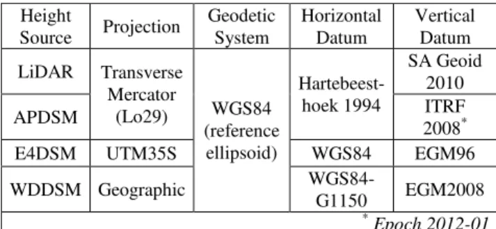
The digital aerial photography, DSM products and lidar data selected for this study utilised different geo-reference systems when originally obtained. The coordinate and geodetic systems that applied to each of the data sources are listed in Table 1.
Table 1. Coordinate and reference systems associated with the obtained height source data
The Lo29 reference system based on the WGS84 reference ellipsoid was the geo-reference framework of choice during this comparative accuracy evaluation. The Elevation4 product was therefore reprojected directly to Lo29 WGS84 using a bilinear method in ESRI software, whilst enforcing strict pixel-to-pixel registration with the gridded reference DEM of matching spatial resolution (‘snap’ raster) in the process. No further positional
x,y-shift was further required with this product. The WorldDEM DSM was similarly co-registered at exactly twelve meter postings, again using bilinear interpolation. The calculation of preliminary displacement vectors and closer visual inspection of the WorldDEM data revealed that a 48 m latitudinal shift directly southwards was required. By subtracting this distance from the raster’s y-coordinates, the DEM was accordingly adjusted horizontally, i.e. ‘bumped’ directly southwards with four pixels. Several software solutions are capable of computing most of the highly complex spatial projections or datum conversions necessary for the sample DEM to achieve proper alignment or co-registration with the reference data. After correctional computations this would produce a reliable orthometric height once the appropriate vertical datum is aligned with the geoidal heights (Chandler and Merry, 2010). To determine the z-offset though, one needs both ellipsoidal height from precise GPS measurements at benchmarks and geoidal height from precise geoidal heights. Ultimately, according to the ASPRS (2013), “it is the client (end user) who must decide whether remaining biases, identified post-delivery, should be removed, or whether they want to avoid the delays and extra cost of removing them”. Since no datum conversions was anticipated from a user’s perspective and because of the co-registration process, the remaining vertical bias, substantially revealed by the preliminary ICPs and the mean relative error of the samples, was removed to expedite the comparative DSM analysis further. Thus, assuming a normal distribution of errors for non-biased datasets, STDDEV and RMSEz will theoretically be the same
when û approaches zero. This was achieved by normalising all three sample DSMs across all cells. Three surface masks at matching grid resolutions were used to eliminate certain pixels beforehand to provide the ultimate z-offset value. The dynamic nature of some off-terrain heights (e.g. tree canopy structure or new buildings) was mitigated by only considering cells at ground (DTM) level. For this purpose a bare surface mask that covered about 77% of the total study region was prepared from the classified laser ground returns. A waterbody mask, rasterised from the digitised vector layer, was used to remove all cells representing physical waterbodies present at the time. The third mask was the extreme outlier constraint set at ±3σ. The uniform z-offset or vertical bias of the Elevation4 DSM was calculated as 7.73 m, for the WorldDEM DSM -0.37 m and the aerial 2 m DSM prototype 0.10 m. Thereafter only the waterbody and outlier constraint masks were again applied to remove the erroneous heights in each unbiased DSM sample before the final error and accuracy metrics of each was computed in both absolute and relative terms as described.
3. EVALUATION RESULTS AND DISCUSSION
3.1 Test 1 – Absolute Vertical Accuracy
The respective absolute accuracy statistics computed for the aerial DSM prototype, the tri-stereo Elevation4 DSM and WorldDEM DSM are shown in Table 2. The ultimate number of ICPs (n) and outliers (N) are also listed accordingly. The differences in absolute vertical accuracy between the three DSM samples were relatively small with only 0.41 m separating the best and worst RMSEz values resulting from the Elevation4 and
WorldDEM samples, respectively. With the overall expected (producer) accuracy descriptor stated for each DSM across all land cover classes, it was clear that all three sample products performed very well. Despite the WorldDEM DSM being the coarsest grid resolution involved, it performed best with regards to the user and producer LE90 accuracy. The tri-stereo DSM Height
Source Projection
Geodetic System
Horizontal Datum
Vertical Datum
LiDAR Transverse Mercator
(Lo29) WGS84 (reference ellipsoid)
Hartebeest-hoek 1994
SA Geoid 2010
APDSM ITRF
2008*
E4DSM UTM35S WGS84 EGM96
WDDSM Geographic
WGS84-G1150 EGM2008
* Epoch 2012-01
basically matched the expected accuracy, whilst the 2 m prototype was marginally beyond the producer accuracy. The selection of absolute accuracy statistics, the variability between LCLU and slope classes and magnitude thereof as computed from the ICPs are presented in the Appendix. Table 1(a) shows these absolute metrics within the relevant LCLU classes. From the resulting graphs one can easily garner that wherever dense natural and/ or alien woody vegetation, urban residential areas with significant canopy cover and, to a lesser degree, commercial or industrial areas were encountered, the error values increased significantly. The same pattern can be observed across all three DSMs, which indicates that it remains challenging to model these complex surfaces with current RS technology (vs laser surveys). Absolute STDDEV and RMSEz
values per LCLU class seldom corresponded closely since the error observations were much less clustered around the (less reliable) positive mean values of ≤ 1 m. The results as assessed across seven different slope classes are shown in Table 1(b). As expected, the error statistics indicate a gradual decrease in accuracy as the slope percentage rise increases. Commercial DEM producers often state the supplied accuracy measure conforms only to slopes < 20% rise, and then supply a separate (larger) statistic for gradients of more than twenty percent (Airbus DS, 2014). These are illustrated by the light-blue shaded areas in the graphs as the expected (producer) accuracy which, in contrast with the expected accuracy measure that was applied uniformly across all LCLU classes involved, caters here for the decrease in accuracy accordingly when negotiating the steeper gradients greater than 20% rise and beyond. The large absolute errors observed in the dense thicket and bush category before has now partly revealed itself (relatively) along the +10% slope classes where large settlement types rarely exist (concurrent to existing building line and land use restrictions) and typically an increase in both natural and alien woody vegetation occurs. The rest of the large absolute error that was realized as the dense urban tree cover are now spread more or less evenly along the moderate to relatively flatter areas (< 5% rise) and in relation to mainly the copious prevailing residential land uses.
DSM Sample
Grid
Size* MAE NMAD RMSEz
User LE90
Prod.
LE90 n N
APDSM 2.0 1.45 0.97 2.06 3.39 3.00 1088 30
E4DSM 4.0 1.42 0.84 1.80 2.96 3.00 1410 37
WDDSM 12.0 1.70 1.26 2.21 3.64 4.00 1424 23 *
All statistical descriptors are in meter units, except n and N
Table 2. Absolute vertical errors and accuracy results for the three DSM samples using ICPs
3.2 Test 2 – Relative Vertical Accuracy
The experimental DSM and the Elevation4 product produced almost identical accuracies with RMSEz values of just below
two metres computed for both. Compared to the absolute LE90 results, the relative accuracy of the base DSM indicated a minor improvement, whilst the tri-stereo DSM fared marginally worse. The coarser WorldDEM performed well again by displaying only slightly larger errors and by maintaining its overall accuracy prediction. A selection of overall relative error and accuracy statistics computed for the three sample DSMs respectively are presented in Table 3. When compared to the results in Test 1, the accuracy values closely followed the same characteristic pattern across all the underlying classes in review. It follows that if one is able to thoroughly measure and report the absolute vertical accuracy, one could have a fair idea of
what relative accuracy to expect from the same 3D data. The relative vertical accuracy results are presented in a similar fashion as Test 1, with Table 2(a) and 2(b) in the Appendix showing the error statistics analysed across the LCLU types and seven slope classes, respectively. The few remaining cells representing waterbodies were the remainder of the resampled LCLU rasters where such (mixed) pixels extended well over the digitised waterbodies at places and can be regarded as insignificant. Because there was now more cells to consider in the Bare/ Mine class than there were ICPs available to determine the absolute error metrics, relatively vertical statistics were more meaningful here. The Cultivation class is where the best vertical accuracy values was obtained in both relative and absolute terms, followed closely by the Wet- and Grassland class and the Woodland/ Open bush classes. As with Test 1, the larger error statistics found in dense natural and/or alien vegetation, and to a lesser extent, urban residential areas with significant canopy cover, were again encountered. Except for these two classes and to some extent the Commercial/ Industrial areas, the STDDEV and RMSEz values were almost identical
measured relatively across the LCLU classes with small, mostly negative mean values. These relative errors thus represent the over (+) or under (-) estimations in height in each LCLU class, and here indicative of the extensive urban canopy cover commonly found here. All three DSM samples performed satisfactorily in the lower to flat gradients (< 5% rise) where the vertical RMSEz values of the stereo and tri-stereo products
measured around 1.75 m. Height underestimations were gradually larger as the percentage slope rise increased, particularly in the case of the WorldDEM. As opposed to the absolute statistics computed in the above 40% slope class, the increased point-to-point count produced more reliable accuracy metrics for that class as reflected by the lower relative values – for the 2 m and 12 m DSMs in particular.
DSM Sample
Grid
Size* û σ MAE RMSEz
User LE90
Prod. LE90 APDSM 2.0 -0.13 1.95 1.36 1.96 3.22 3.00
E4DSM 4.0 -0.22 1.97 1.38 1.98 3.26 3.00
WDDSM 12.0 -0.47 2.16 1.59 2.21 3.63 4.00 *
All statistical descriptors are in meter units
Table 3. Relative vertical errors and accuracy results for the three DSM samples using reference surfaces
3.3 Test 3 – Relative Horizontal Accuracy
The error metrics and results from all the horizontal accuracy computations of the DSMs samples involved after blunders (N) were removed are summarised in Table 4. The horizontal user LE90 accuracies computed for the 2 m base DSM sample, the Elevation4 DSM and the WorldDEM DSM sample were all better than the producer estimates. Each DSM performed well with the overall user error and grid size ratio being around one to one-and-half pixel.
DSM Sample
Grid
Size* MDL MAD RMSE
r
User LE90
Prod.
LE90 n N
APDSM 2.0 2.14 1.01 2.21 3.35 4.00 255 13
E4DSM 4.0 4.30 1.78 3.65 5.54 6.00 126 8
WDDSM 12.0 12.80 4.22 6.00 9.11 10.00 72 0 *
All statistical descriptors are in meter units, except n and N
Table 4. Relative horizontal errors and accuracy results for three DSM samples using computed displacement vectors (DVs) ISPRS Annals of the Photogrammetry, Remote Sensing and Spatial Information Sciences, Volume IV-2/W1, 2016
3.4 Final Remarks and Conclusion
This study was concerned with testing local DSM quality in order to address a dire need for high resolution elevation data in South Africa. Conducted over part of the City of Tshwane, three alternatives to the incomplete national DEM was investigated. The overall accuracy results indicated that the 2 m DSM prototype constructed from aerial stereo-pairs, the tri-stereo Elevation4 product and global WorldDEM DSM sample all comfortably met their proclaimed geo-positional accuracy criteria. The good performance shown by the experimental baseline DSM was very encouraging by closely emulating the tri-stereo product. The prototype demonstrated that it is feasible to consider its realisation at 2 m to 4 m postings over the entire country to obtain a good quality baseline DSM. By achieving the second best absolute vertical RMSEz and best relative
RMSEz results, the experimental DSM performed very similar
to the 4 m tri-stereo product as intended. However, the digital aerial photographs will serve a national purpose only with no (similar) height data available to mesh with seamlessly once the country’s international borders are reached with its six neighbours. The Elevation4 tri-stereo product was the best performer in terms of absolute RMSEz and basically as accurate
as the 2 m prototype relative to its co-registered reference surface. The HRSI system provided by the Pléiades satellite constellation thus offers an attractive ortho-optic data option, especially when considering the large swath on hand, agility and reactivity for large surface area surveys. The Pléiades’ 400 km2 large footprint could cover the entire study region with ease during the tri-stereo acquisitions. Similarly operational like the Pléiades constellation, the Tandem-X mission poses novel InSAR technology to measure and monitor larger across-border phenomena, yet largely irrespective of cloud cover – the optic sensor’s constant adversary in parts of this country. It is in this context that the quality of the WorldDEM DSM product is truly remarkable when considering its global coverage. It resembles a DEM system where both the DSM and DTM are regarded as vital 3D products necessary to support routine small to large scale city planning, civil engineering and other related specialist 3D tasks and investigations. Although it seems that the model cannot resolve minor local variation in topography as well as the previous two DSM samples when appraising its accuracy results, the original support cell size is much smaller than the product’s 12 m resolution. Adding newly collected InSAR data and routinely upscaling the data will no doubt continue to improve the model over time, as well as deal more effectively with steep surface gradients. Both space borne commercial DSM alternatives above unfortunately remain high cost options at present for the country. Nonetheless, the impact that all three these very useful 3D data sources and topographic representations will make in the local geomorphometry domain is almost evident. Other than contributing to an improved standard of orthorectification (Henrico et al., 2016), it would certainly also advance most image processing, classification or segmentation and change detection techniques. It could also benefit scientific biomass and hydrological investigations that came to the fore more prominently here and elsewhere, but which lack quality spatial data or 3D details.
ACKNOWLEDGEMENTS
The author would like to thank the City of Tshwane and AAM Geomatics for permitting the CSIR to freely utilise the lidar data and metadata; the CD:NGI in Mowbray, Cape Town for the basic free use of their expansive archived aerial photography resources; Airbus Defence and Space for supplying the
WorldDEM™ sample for this assessment permissible under a Technical Evaluation License Agreement with the CSIR; and finally GeoTerra Image™ for the GTI National Land Cover 2013/14 dataset supplied in agreement to its open licence status and standard EULA.
REFERENCES
Airbus DS, 2014. Technical Product Specification, Version 1.0, Geo-Intelligence Programme, April 2014, Airbus Defence and Space, Toulouse, France, pp. 1-33.
Al-Durgham, M., Fotopoulos, G. and Glennie, C., 2010. On the accuracy of LiDAR derived digital surface models. In: Mertikas, S.P. (ed.), Gravity, geoid and earth Observation, International Association of Geodesy Symposia 135, Springer-Verlag, Berlin pp. 689-695.
ASPRS, 2013. American Society of Photogrammetry and Remote Sensing Accuracy Standards for Digital Geospatial Data, Photogrammetric Engineering & Remote Sensing, December 2013, pp. 1073-1085.
CD:NGI, 2010. National Standard for the Acquisition of Digital Aerial Imagery (QLAS.SD.2_v1_2010.12.14.doc), Chief Directorate: National Geospatial Information, Mowbray, Cape Town, South Africa.
Chandler, G., and Merry, C., 2010. The South African Geoid 2010: SAGEOID10. PositionIT, June 2010, EE Publishers, Muldersdrift, South Africa, pp. 29-33.
Coeurdevey, L., and Gabriel-Robez, C. 2012. Pléiades Imagery - User Guide, Technical Report No. USRPHR-DT-125-SPOT-2.0, October, 18, 2012 http://www.intelligence-airbusds.com/en/4555-pleiades-user-guide (22 June 2016).
Da Costa, J.K.N., 2010. Geometric quality testing of the WorldView-2 image data acquired over the JRC Maussane Test Site using ERDAS LPS, PCI Geomatics and Keystone digital photogrammetry software packages – Inital Findings. Scientific and Technical Research Series, ISSN 1018-5593, Publications Office of the EU, Luxembourg, pp. 1-25.
Demir, N., Poli, D., and Baltsavias, E., 2009. Combination of image and LiDAR data for building extraction. Proceedings of the 9th Conference on Optical 3D Measurement Techniques, 1-3 July, 2009, Vienna, Austria, pp. 1-10.
Doytsher, Y., Dalyot, S., and Katzil, Y., 2009. Digital terrain models: a tool for establishing reliable and qualitative environmental control processes. In: De Amicis, R. et al. (eds.), GeoSpatial Visual Analytics: Geographical Information Processing and Visual Analytics for Environmental Security, Springer-Verlag, Berlin, pp. 215-234.
Fisher, P.F., and Tate, N.J., 2006. Causes and consequences of error in digital elevation models. Progress in Physical Geography 30, pp. 467-489
GEOTERRAIMAGE, 2014. 2013 - 2014 South African National Land Data User Report and MetaData, February 2015, v.05, GEOTERRAIMAGE, Pretoria, South Africa, pp. 1-53.
Grohmann, C.H,, Sawakuchi, A.O., and Mendes, V.R., 2011. Cell size influence on DEM volume calculation. Proceedings of Geomorphometry 2011, 7-9 September 2011, ESRI Campus Redlands, Los Angeles, USA, pp. 63-66.
Hajnsek, I., Busche, T., Krieger, G., Zink, M., Schulze, D., and Moreira, A., 2014. Announcement of Opportunity: TanDEM-X Science Phase. Doc.: TD-PD-PL-0032, Issue: 1.0, 19.05.2014, TanDEM-X Ground Segment, Microwaves and Radar Institute (DLR-HR), Germany, pp. 1-27.
Henrico, I., Breytenbach, A., and Combrinck, L., 2016. Accuracy comparison of ortho-images by alternating the number of GCPs and elevation sources. South African Journal of Geomatics, (in print), pp. 13.
Hirt, C., Filmer, M.S., and Featherstone, W.E., 2010. Comparison and validation of the recent freely available ASTER-GDEM ver1, SRTM ver4.1 and GEODATA DEM-9S ver3 digital elevation models over Australia. Australian Journal of Earth Sciences 57, pp. 337-347.
Hengl, T., and Reuter, H., 2011. How accurate and usable is GDEM? A statistical assessment of GDEM using LiDAR data. Proceedings of Geomorphometry 2011, 7-9 September 2011, ESRI Campus Redlands, Los Angeles, USA, pp. 45-48.
Hengl, T., and Evans, I.S., 2009. Mathematical and digital models of the land surface. In: Hengl, T. and Reuter, H.I. (eds.), Developments in Soil Science 33, Elsevier, Amsterdam, Netherlands, pp. 31-63.
Höhle, J., and Höhle, M., 2009. Accuracy assessment of digital elevation models by means of robust statistical methods. ISPRS Journal of Photogrammetry and Remote Sensing 64, pp. 398-406.
Hutchinson, M.F., Xu, T., and Stein, J.A., 2011. Recent progress in the ANUDEM elevation gridding procedure. In: Geomorphometry 2011, Hengel, T., Evans, I.S., Wilson J.P., and Gould, M. (eds.), Redlands, California, USA, pp. 19-22.
Krauss, T., and Reinartz, P., 2010. Enhancement of dense urban digital surface models from VHR optical satellite stereo data by pre-segmentation and object detection. Proceedings of the ISPRS COM I Symposium "Image Data Acquisition – Sensors & Platforms", 15-18 June, 2010, Calgary, Canada.
Krieger, G., Moreira, A., Fiedler, H., Hajnsek, I., Werner, M., Younis, M., and Zink, M., 2010. TanDEM-X: A satellite formation for high resolution SAR interferometry. IEEE Transactions on Geoscience and Remote Sensing, 45(11), pp. 3317–3341.
Krieger, G., Zink, M., Bachmann, M., Bräutigam, B., Schulze, D., Martone, M., Rizzoli, P., Steinbrecher, U., Walter A.J., De Zan, F., Hajnsek, I., Papathanassiou, K., Kugler, F., Rodriguez C.M., Younis, M., Baumgartner, S., Lopez Dekker, P., Prats, P., and Moreira, A., 2013. TanDEM-X: A radar interferometer with two formation flying satellites. Acta Astronautica, Elsevier, Vol. 89, pp 83-98.
Maune, D.F., Maitra, J.B., and McKay, E.J., 2007. Accuracy standards and guidelines. In: Digital Elevation Model Technologies and Applications: The DEM User’s Manual, 2nd ed., Maune, D. (ed.), Bethesda, American Society for Photogrammetry and Remote Sensing, pp. 65-97.
Milevski, I., Gorin, S., Markoski, B., and Radevski, I., 2013. Comparison of accuracy of DEM’s available for the Republic of Macedonia. In: Efe, R., Atalay, I., Cürebal, I. (eds.) GEOMED
2013. Proceedings of the 3rd International Geography Symposium, 10-13 June 2013, Antalya, Turkey, 165-172.
Mitchell, A., 2005. The ESRI Guide to GIS Analysis, Vol. 2, ESRI Press, Redlands, California, USA, pp. 1-252.
Nelson, A., Reuter, H.I., and Gessler, P., 2009. DEM production methods and sources. In: Hengl, T. and Reuter, H.I. (eds.), Developments in Soil Science 33, Elsevier, Amsterdam, Netherlands, pp. 65-85.
Oh, J.H., 2011. Novel approach to epipolar resampling of HRSI and satellite stereo imagery-based georeferencing of aerial images. Unpublished PhD Dissertation. Columbus, Ohio State University, USA, pp. 1–93.
PCI Geomatics, 2013. OrthoEngine Training Manual, Geomatica OrthoEngine Course Exercises Version 2013 http://www.pcigeomatics.com/pdf/OrthoEngine_CourseGuide_ 2013.pdf (02 Nov. 2016).
Poli, D., Wolff, K. and Gruen, A., 2009. 3D geodata recovery from high resolution satellite imagery. In: Proceedings of the 33rd International Symposium on Remote Sensing of Environment, Sustaining the Millennium Development Goals, May 2009, Ispra, Italy, Vol. 1, Part 2, pp. 1081-1085.
Pulighe, G., and Fava, F., 2013. DEM extraction from archive aerial photos: accuracy assessment in areas of complex topography. European Journal of Remote Sensing, 46, pp. 363-378.
Reuter, H.I. and Kersebaum, K.C., 2009. Applications in precision agriculture. In: Hengl, T. and Reuter, H.I. (eds.), Developments in Soil Science 33, Elsevier, Amsterdam, Netherlands, pp. 623-636.
Reuter, H.I,. Hengl, T., Gessler, P., and Soille, P., 2009. Preparation of DEMs for geomorphometric analysis. In: Hengl, T. and Reuter, H.I. (eds.), Developments in Soil Science 33, Elsevier, Amsterdam, Netherlands, pp. 87-120.
Rexer, M., and Hirt, C., 2014. Comparison of free high-resolution digital elevation data sets (ASTER 1 GDEM2, SRTM v2.1/v4.1) and validation against accurate heights from the Australian National 2 Gravity Database. Australian Journal of Earth Sciences 2014, pp 1-15.
Tinkham, W.T., Smith, A.M.S., Hoffman, C., Hudak, A.T., Falkowski, M.J., Swanson, M.E., and Gessler, P.E., 2012. Investigating the influence of LiDAR ground surface errors on the utility of derived forest inventories. Tecnical Report 182, USDA Forest Service, Lincoln Faculty Publications, University of Nebraska, USA, pp. 1-12.
Van Niekerk, A., 2015. Stellenbosch University Digital Elevation Model (SUDEM), 2015 Edition, Technical report DOI: 10.13140/RG.2.1.1795.6324 http://146.232.21.108/ Downloads/sudem/SUDEM_Product_Description.pdf (08 April 2016).
Van Niel, T.G., McVicar, T.R., Li, L.T., Gallant, J.C., and Yang, Q.K., 2008. The impact of misregistration on SRTM and DEM image differences, Remote Sensing and Environment 112(5), pp. 2430-2442.
APPENDIX