Pages: 186-194 DOI: 10.13057/biodiv/d150210
Spatial gradients in freshwater fish diversity, abundance and current
pattern in the Himalayan region of Upper Ganges Basin, India
AJEY KUMAR PATHAK, UTTAM KUMAR SARKAR♥, SHRI PRAKASH SINGH
National Bureau of Fish Genetic Resources, Canal Ring Road, Post - Dilkusha, Lucknow 226002, Uttar Pradesh, India. Tel: +91-5222442440, Fax: +91-5222442403,♥email: [email protected]
Manuscript received: 3 June 2014. Revision accepted: 10 July 2014.
ABSTRACT
Pathak AK, Sarkar UK, Singh SP. 2014. Spatial gradients in freshwater fish diversity, abundance and current pattern in the Himalayan region of Upper Ganges Basin, India. Biodiversitas 15: 186-194.The present study describes the analysis and mapping of the different measurements of freshwater fish biodiversity of the Upper Ganges basin in the Himalayan region using spatial interpolation methods of Geographical Information System. The diversity, richness and abundance of fishes for each sampling location were determined and Kriging interpolation was applied on each fisheries measurement to predict and produce semivariogram. The semivariogarms produced were cross validated and reclassified. The reclassified maps for richness, abundance and diversity of fishes, occurrence of cold water threatened fish and abundance of important genera like Tor, Schizothorax and species were produced. The result of the Kriging produced good results and overall error in the estimation process was found significant. The cross validation of semovariograms also provided a better result with the observed data sets. Moreover, weighted overlay analysis of the reclassified raster maps of richness and abundance of fishes produced the classified raster map at different evaluation scale (0-10) qualitatively describing the gradient of species richness and abundance compositely. Similarly, the classified raster map at same evaluation scale qualitatively describing the gradient of species abundance and diversity compositely was produced and published. Further, basin wise analysis between Alaknanda/Pindar and Ganga1 sub basins showed 0.745 disparities at 0.745 distances in 2 dimensional spaces. The richness, diversity and abundance of threatened fishes among the different sampling locations were not significant (p = 0.9).
Key words:Fish diversity, GIS, Himalayan region, India, spatial gradients, Upper Ganga basin.
INTRODUCTION
The freshwater biodiversity is declining at an alarming rate, far greater than that which has been noted for even the most affected terrestrial systems (Dudgeon et al. 2006). Additionally, global warming, climate change (Buisson et al. 2008) extreme weather, natural and man-made pollution, overharvesting, overexploitation, invasion of exotic fishes (Dudgeon et al. 2006) and other human disturbances have also much impacted on the fish biodiversity (Lipsey and Child 2007). Thus, in order to develop and test hypotheses about the processes responsible for this decline and to set conservation priorities, it is essential to understand the pattern of spatial variation in diversity (Fischer and Paukert 2008; Wu et al. 2011).
In India, the Ganges basin is one of the most valuable resources of biotic diversity and it is one of the most populated river basin in the world, with over 400 million people and a population density of about 1,000 inhabitants per square mile (390/km2) (Arnold 2000). The flow of many tributaries of the Ganges has been diverted and controlled by barrages for irrigation due to which the fish catch has been declined and caused loss of species diversity (Das 2007; Payne et al. 2004; Sarkar et al. 2013). Twenty nine freshwater fish species recorded from the river Ganges
have been listed as threatened under vulnerable and endangered categories (Lakra et al. 2010). The fish fauna of the Ganges river and its tributaries have been studied by several researchers and information generated was mostly based on the taxonomy, biogeographical distribution and ecological aspects (e.g., Hamilton 1822; Hora 1929; Day 1888; Krishnamurti et al. 1991; Bilgrami and Datta-Munshi 1985; Srivastava 1980; Revenga and Mock 2000; Sinha 2006; Payne et al. 2004; Sarkar et al. 2010, 2012). Such information is insufficient to address the critical issues pertaining to conservation and management of fish diversity in the Ganges due to the mounting tendency of different threats. Therefore, conservation and restoration of rivers have become imperative for overall fisheries development, ecological integrity as well as livelihood security for the local community.
and underlying habitat characteristics for management and restoration, managing resources and many more. Identification of critical habitat is a priority for many fisheries managers, especially those trying to manage large river fisheries resources (Raibley et al. 1997). The value of GIS to fisheries professionals is that it allows for 3-D visualization with correct spatial features and attributes for each point. Previous analysis of fisheries data did not permit the analysis of spatial data in three dimensions.
Thus, in view of the above, the present study was planned to spatially document, analyze and map different fisheries measurements using the techniques of GIS. The present paper discusses the different statistical and geostatistical methods used in analyzing and mapping the different fisheries measurements (richness, diversity and abundance) in the Himalayan region of the upper Ganga basin.
MATERIAL AND METHODS
Data sources and collection
The data on fish was collected according to the methodology described by Sarkar et al. (2012) by sampling into the main channel and selected tributaries of Alaknanda/Pindar and Ganga1 sub basins. Figure 1 presents the collection map of sampling locations and Table 1 presents the list of sampling locations in the different rivers covered in each district. Geographic Positioning System (GPS) was used to record the geographical position of the sampling points. The satellite image from LISS III sensor of Indian Remote Sensing Satellite (IRS) was used to delineate the rivers and tributaries. Toposheets from Survey of India (SOI), Dehradun was used for geometric correction of the satellite image. Administrative Boundary Database procured from SOI, Dehradun was used for extracting the administrative boundaries.
Figure 1. Fish sample collection map of locations in Uttarakhand, India
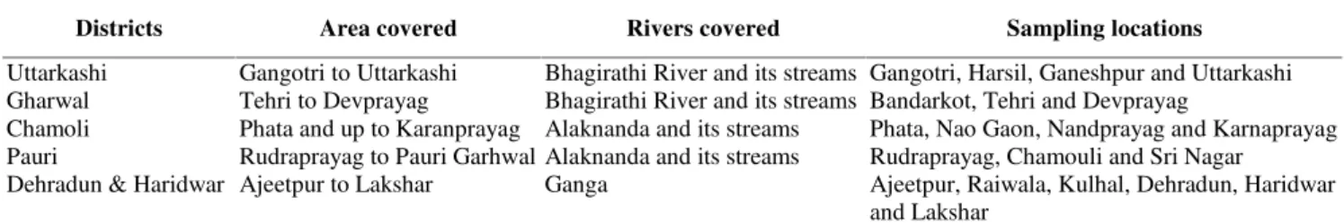
Table 1. List of sampling locations in the different rivers passing through the districts of Uttarakhand, India
Districts Area covered Rivers covered Sampling locations
Uttarkashi Gangotri to Uttarkashi Bhagirathi River and its streams Gangotri, Harsil, Ganeshpur and Uttarkashi Gharwal Tehri to Devprayag Bhagirathi River and its streams Bandarkot, Tehri and Devprayag
Chamoli Phata and up to Karanprayag Alaknanda and its streams Phata, Nao Gaon, Nandprayag and Karnaprayag Pauri Rudraprayag to Pauri Garhwal Alaknanda and its streams Rudraprayag, Chamouli and Sri Nagar
Dehradun & Haridwar Ajeetpur to Lakshar Ganga Ajeetpur, Raiwala, Kulhal, Dehradun, Haridwar
Specimen and fish data analysis
The collected specimens from each sampling location were identified by following Jayaram (1999) and Sarkar et al. (2012). The fish diversity for each sampling location was calculated using the following formula suggested by Shannon and Wiener (1963).
n i N ni N ni H 1 2 logWhere H = Shannon-Wiener index of diversity; ni = total numbers of individuals of species,N = total number of individuals of all species.
The threatened status categories for the identified fish species was determined by following the IUCN Red List criteria and the percentage relative abundance of the threatened fishes for each sampling location was calculated.
Spatial data set preparation and analysis
ESRI's ArcGIS ArcINFO 10 (ESRI 2014) and PCI's Geomatica 10 (PCI Geomatics 2006) software was used to prepare the GIS based vector base map covering rivers, administrative boundaries and sub basins derived from geometrically corrected satellite image from LISS III sensor, Administrative boundary database and Hydro 1K data sources. A point vector layer for sampling points using GPS was created and arranged on the base map. The table of the point vector layer was populated with fish and fisheries measurement data. ESRI’s ArcGIS Geostatistical
Analyst Software (GAS), which provides an extensive set of interpolation tools, was used to interpolate the fisheries measurement data. Though this software includes different interpolation methods that allows predictions of unknown values of a random function from observations at known locations, the present study describes the Kriging interpolation method, which was applied for spatial prediction and mapping. For interpolation and calculation of spatial autocorrelation statistics, the study area was divided into30 minute interval and grid cells were assigned to the cell centroid. All data were analyzed in the Polyconic projection. The projection was necessary to ensure that the value of x and y units is equivalent and constant across the study region. The spatial mapping process consisted of sequence of operations: creation of spatial weight matrix for checking spatial autocorrelation of different fisheries measurements; selection of geostatistical method for interpolation; fitting the best model; generation of semivariogram; cross validation and publishing.
RESULTS AND DISCUSSION
Statistical analysis of fisheries measurements
A total of 50 species belonging to 33 genus and 14 families were recorded. The analysis of the fish data showed that 22 species belong to Alaknanda/ Pindar and 42 species in Ganga1 sub basin, 13 species were found common in both the sub basins. Table 2 provides the list of
species recorded in these two sub basins and Figure 2 provides the scatter plot of the species.
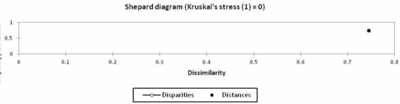
Further proximity analysis between the sub basins showed 0.745 dissimilarity. The result of the proximity analysis using the Jaccard's coefficient has been presented in Table 3. This dissimilarity was observed at 0.745 disparity/ distance in two dimensional spaces when
Table2. List of fish species collected from the different sampling locations of different rivers (1-presence and 0 -absence)
Fish species Alaknanda/Pindar Ganga1
Amblyceps mangois 0 1
Barilius barila 1 0
Barilius bendelisis 1 1
Barilius tileo 0 1
Barilius vagra 1 0
Botia lohachata 1 0
Catla catla 0 1
Chagunius chagunio 0 1
Channa marulius 0 1
Channa striatus 0 1
Chela cachius 0 1
Chitala chitala 0 1
Cirrhinus mrigala 1 0
Cirrhinus reba 0 1
Crossocheilus latius 0 1
Cyprinus carpio 1 0
Glyptothorax sp. 1 1
Glyptothorax telchitta 0 1
Heteropneustes fossilis 0 1
Labeo bata 1 1
Labeo calbasu 1 0
Labeo dyocheilus 1 1
Labeo pangusia 0 1
Labeo rohita 0 1
Macrognathus aral 1 0
Mastacembelus armatus 0 1
Nemacheilus beavani 1 1
Nemacheilus botia 1 1
Nemacheilus corica 0 1
Nemacheilus montanus 1 0
Nemacheilus rupicola 0 1
Ompok pabda 0 1
Oncorhynchus mykiss 1 0
Puntius chelynoides 1 1
Puntius ticto 0 1
Rasbora daniconius 1 1
Rita rita 0 1
Salmophasia bacaila 0 1
Schizothorax curvifrons 0 1
Schizothorax progastus 1 1
Schizothorax richardsonii 1 1
Schizothorax sinuatus 0 1
Setipinna phasa 0 1
Silonia silondia 0 1
Sperata aor 0 1
Tetraodon fluviatilis 0 1
Tor putitora 1 1
Tor tor 1 1
Wallago attu 0 1
Xenentodon cancila 0 1
Figure 2. Scatter plot of fish species between Alaknanda/ Pindar and Ganga1 sub basin.
Figure 4. Shepard diagram showing disparities and distnace between Alaknanda/Pindar and Ganga1 subbasins.
multidimensional scaling (MDS) of the proximity was performed. Figures 3 and 4 presents the Configuration and Shepard diagram after performing the MDS analysis using Kruskal's stress (1). Tables 4 and 5 summarize the result of descriptive statistics and correlations. Further, ANOVA single factor analysis of the sampling locations at 95% confidence level on the species richness, fish diversity index and abundance of threatened fish species was done and the pvalue was found not significant (Table 6).
Geostatistical analysis and mapping
The spatial autocorrelation of different fisheries measurements like index of fish diversity, species richness and abundance, abundance of threatened fishes, abundance of Tor and Barilius species showed that the spatial distribution of feature values is the result of random spatial processes as the computed value of p was found not statistically significant. Thus, the observed spatial pattern of feature values could very well be one of many, many possible versions of complete spatial randomness (CSR). The p value (0.013) in the spatial autocorrelation of abundance of genusSchizothorax species was statistically significant and the z score (2.473) was found positive. This result showed that the null hypothesis could be rejected and the spatial distribution of high values and/or low values in the dataset is more spatially clustered than would be expected if underlying spatial processes were random. Further, the composite evaluation of the species richness and abundance was done using the overlay weighted
Table 3.Species frequency and percentage in Alaknanda/ Pindar and Ganga1 subbasins (A); Similarity/ Proximity matrix between Alaknanda/ Pindar and Ganga1 subbasins (B)
A. Summary statistics:
Variable Categories Freq. Perc.
Alaknanda/Pindar 0 29 56.863
1 22 43.137
Ganga1 0 9 17.647
1 42 82.353
B. Proximity matrix (Jaccard coefficient):
Alaknanda/Pindar Ganga1
Alaknanda/Pindar 1 0.255
Ganga1 0.255 1
Table 4. Descriptive statistics of the sampling locations on the variables species richness, fish diversity index and abundance of threatened fish species.
Parameters Species
richness
Index of fish diversity
Abundance of threatened fish
species (%)
Mean 6.16 0.09 1.16
SE 0.93 0.03 0.16
Median 4 0.03 1.34
Mode 3 0.01 0
SD 4.66 0.17 0.81
SV 21.8 0.03 0.65
Kurtosis 3.62 19.51 -0.82
Skewness 1.95 4.22 -0.18
Range 19 0.879 2.67
Min. 2 0.012 0
Max. 21 0.891 2.67
Sum 154 2.42 29.22
Count 25 25 25
Largest (1) 21 0.89 2.67
Smallest (1) 2 0.012 0
Note: SE = Standard Error, SD = Standard Deviation, SV = Sample Variance, Min. = Minimum, Max. = Maximum.
Table 5.Degree of correlation among the sampling locations on the variables species richness, fish diversity index and abundance of threatened fish species.
Variables species
richness Index of fish diversity Abundance of threatened fish species (%)
Species richness 1.000 0.813 0.797
Index of fish diversity 0.813 1.000 0.546 Abundance of threatened
fish species (%)
0.797 0.546 1.000
Table 6.The result of ANOVA among sampling sites on species, index of fish diversity and relative abundance of threatened fish species.
Source of Variation
SS df MS F P-value F crit
Between groups
240.1535 24 10.0064 0.607749 0.906785 1.73708 Within
groups
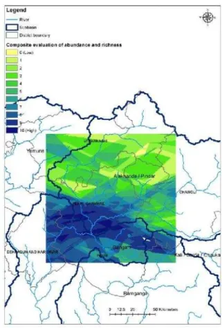
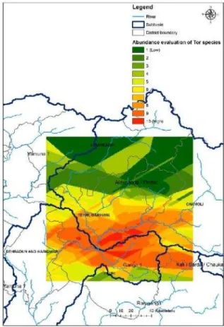
analysis of the classified cross validated raster maps of species richness and abundance produced after the Kriging interpolation (Figure 5) and the study indicated that upper part of the Ganga1, upper northern part of Ramganga and southern lower part of the Alaknanda form the greater composition of species richness and abundance. Similarly, the composite evaluation of species abundance and index of fish diversity (Figure 6) showed that upper northern part of Ganga1 and middle and lower southern part of Alaknanda/ Pindar sub basins have greater composition in terms of abundance and diversity. The semivariogram map produced after application of Kriging interpolation methods on the abundance of threatened fish species (Figure 7) indicates that upper part of Ganga1 and Ramganga sub basins are relatively important for more abundance of threatened fish species. The analysis of semivariogram map produced after Kriging interpolation methods for abundance ofSchizothorax species (Figure 8) revealed that the species are abundantly colonized in the middle and upper part of Alaknanda/ Pindar, north eastern upper part of Ganga1 and upper northern part of the Ramganga sub basin. The semivariogram map of Tor species (Figure 9) showed the high degree of abundance in Alaknanda/Pindar, Ganga1 and upper northern part of Ramganga. The abundance distributional range of this species was found fairly larger than Schizothorax species. Similarly, the abundance of Barilius species (Figure 10) was noticed relatively more in Ganga1. The lower southwestern part of Alaknanda adjacent to Ganga1 basin also showed a high degree of abundance ofBarilius species.
Discussion
Planning the conservation of freshwater fish biodiversity at regional scale requires mapped information on current patterns of fish diversity and conservation targets at a relatively fine scale (Fitz-Hugh 2005). Hence, many of the GIS based studies represented a major step in defining patterns of freshwater biodiversity and identifying freshwater conservation priorities in some areas of the world (Higgins et al. 2003; Weitzell et al. 2003; Januchowski-Hartley et al. 2011). The present study demonstrates the changing pattern of different fisheries measurements and hardly significant differences were observed between predicated and observed values. Sources of variability in our observed data stem from the inefficiency of capture, and less number of sampling points. The prediction accuracy was found satisfactory and more promising for all the fisheries measurements. Further, gradients in abundance of important genera (Schizothorax,
TorandBarilius species),showed that areas of abundance predicted by the used model are correct and justifies the studies (Nautiyal et al. 1998). The high abundance of
Schizothorax species was noticed in Alaknanda/Pindar sub basin while the high abundance ofTor species was noticed both in Alaknanda/Pindar and Ganga1 sub basins. Similarly, the high abundance of Barilius species was noticed in the Ganga1 sub basin only. At very high altitudes, the model predicted the very meager abundance of Tor andBarilius species while on the other hand the abundance ofSchizothorax species was predicted relatively
Figure 5. Classified interpolated raster map of species abundance and richness
Figure 7. Classified interpolated raster map of the abundance of threatened fishes
Figure 8. Classified interpolated raster map of the abundance of
Schizothorax species
Figure 9. Classified interpolated raster map of the abundance of
Torspecies
Figure 10. Classified interpolated raster map of the abundance of
high which again justifies the studies. Thus, this model presents the areas of conservation value with reference to
Schizothorax, Torand Barilius species and also the areas where high species diversity was noticed. The comparative evaluation showed that Ganga1 is better than southern part of Alaknanda/Pindar sub basin. Similarly, Ganga1 again showed the better enrichment in terms of species richness and abundance. Further, results on the abundance of threatened fishes indicated that these are fairly distributed in the tributaries of the main channels of all three sub basins. Therefore, effective conservation and prioritization of potential sites of the fish biodiversity could be planned in the areas as the model presents the areas of key locations within the river basin at spatial scale. The GIS tools have been instrumental to incorporate freshwater biodiversity into its eco-regional assessment process, because they can efficiently produce the necessary output products using widely available GIS datasets (Fitz-Hugh 2005).
CONCLUSION
Our study concerns essentially with diversity, abundance and distribution pattern of freshwater fish species in the upper Ganges, but it posits an important challenge to the domains and the respective key drivers that play an important role behind these patterns. The unprecedented river flow regulation for hydropower generation, disturbances in landscape habitat, introduction of exotic fish species are some noticeable key drivers in the Upper Ganga basin. In the Himalaya water discharge was found one of the key drivers behind diversity and distribution pattern. Thus, with reference to Upper Ganga basin in the Himalayan region, there is an urgent need to correlate the fish diversity data with landscape scale habitat pattern and attributes, river flow and other disturbances like damming in order to classify the suitable fish habitat and predict the fish distribution for better management decision. The present study suggests determining the spatial pattern of diversity, abundance and distribution of species in relation to landscape habitat variables. Indeed, this could be one of the local specific models for prioritization of sites for conservation and management of fish biodiversity with reference to upper Ganges which is a highly sensitive ecosystem.
ACKNOWLEDGEMENTS
The authors are grateful to the Director, NBFGR, Lucknow, Uttar Pradesh, India for providing necessary facilities and suggestions.
REFERENCES
Arnold G. 2000. World strategic highways. Taylor & Francis, New York. Bilgrami KS, Datta-Munshi JS 1985. Ecology of River Ganges
(Patna-Farakka); impact of human activities and conservation of aquatic biota. Final Technical Report, Department of Environment Research Project under MAB Programme, India.
Buisson L, Thuiller W, Lek S, Lim P, Grenouillet G. 2008. Climate change hastens the turnover of stream fish assemblages. Glob Chang Biol 14: 2232-2248.
Das MK, Samanta S, Saha PK. 2007. Riverine health and impact on fisheries in India. Policy Paper No. 01, Central Inland Fisheries Research Institute, Barrackpore, Kolkata.
Day F. 1888. The Fishes of India; being a natural history of the fishes known to inhabit the seas and fresh waters of India, Burma and Ceylon. Williams and Norgate, London. [Digitizing by Harvard University, Museum of Comparative Zoology, Ernst Mayr Library; available at https://archive.org/details/fishesofindiabei03dayf] Dudgeon D, Arthington AH, Gessner MO, Kawabata ZI, Knowler DJ, et
al. 2006. Freshwater biodiversity: Importance, threats, status and conservation challenges. Biol Rev 81: 163-182.
ESRI. 2014. ArcGIS® 10.2.1 for Desktop Functionality Matrix. ESRI, New York. http://www.esri.com/software/arcgis/arcgis-for-desktop Fischer JR, Paukert CP. 2008. Habitat relationships with fish assemblages
in minimally disturbed Great Plains regions. Ecol Freshw Fish 17: 597-609.
Fitz-Hugh TW. 2005. GIS tools for freshwater biodiversity conservation planning. Trans in GIS 9(2): 247-263.
Hamilton F. 1822. An account of the fishes found in the river Ganges and its branches. Printed for A. Constable and company, Edinburgh. Higgins JV. 2003. Maintaining the ebbs and flows of the landscape:
Conservation planning for freshwater ecosystems. In Groves CG (ed)
Drafting a Conservation Blueprint: A Practitioner’s Guide to Planning
for Biodiversity. Island Press, Washington, DC.
Hora SL. 1929.An aid to the study of Hamilton-Buchanan’s ‘‘Gangetic fishes’’. Mem Indian Mus 9: 169-192
Januchowski-Hartley SR, Pearson RG, Puschendrf R, Rayner T. 2011. Freshwaters and Fish diversity: Distribution, protection and disturbance in tropical Australia. PLOS One 6 (10): e25846.DOI: 10.1371/journal.pone.0025846
Jayaram KC. 1999. The freshwater fishes of the Indian region. Narendra Publishing House, India
Krishnamurti CR, Bilgrami KS, Das TM, Mathur RP. 1991. The Ganga, a scientific study. Ganga Project Directorate. Northern Book Center, New Delhi.
Lakra WS, Sarkar UK, Gopalakrishnan A, Pandian AK. 2010. Threatened freshwater fishes of India. NBFGR Publication, Lucknow, India. Lipsey MK, Child MF. 2007. Combining the fields of reintroduction
biology and restoration ecology. Conserv Biol 21: 1387-1388. Nautiyal P, Bhatt JP, Rawat VS, Kishor B, Nautiyal R, Singh HR. 1998.
Himalayan Mahseer: Magnitude of commercial 1030 fishery in Garhwal hills. Fish Genet Biodiv Conserv Nat in Pub 5: 107-114. Payne AI, Sinha RK, Singh HR, Haq S. 2004. A review of the Ganges
Basin: its fish and fisheries. In: Welcomme RL, Peter T (eds) Proceedings of the Second International Symposium on the Management of Large Rivers for Fisheries, vol 1, FAO Regional Office for Asia and the Pacific, Bangkok, Thailand.
PCI Geomatics. 2006. Geomatica 10.0.3. PCI Geomatics, Ontario, CA. www.pcigeomatics.com
Raibley PT, Irons KS, O'Hara TM, Blodgett KD, Sparks RE. 1997. Winter habitats used by largemouth bass in the Illinois River, a large river-floodplain ecosystem. North American J Fish Manag 17: 401-412. Revenga C, Mock G. 2000. Pilot Analysis of global ecosystems:
freshwater systems and world resources 1998-99. World Resources Institute, Washington, DC.
Sarkar UK, Gupta BK, Lakra WS. 2010. Biodiversity, eco-hydrology, threat status and conservation priority of the freshwater fishes of river Gomti, a tributary of river Ganga (India). Environmentalist 30 (1): 3-17.
Sarkar UK, Pathak AK Sinha RK, Sivakumar K., Pandian AK, Pandey A, Dubey VK, Lakra WS. 2012. Freshwater fish biodiversity in the River Ganga (India): Changing pattern, threats and conservation perspectives. Rev Fish Biol Fish 22: 251-272.
Shannon CE, Wiener W. 1963. The mathematical theory of communication. University of Illinois Press, Urbana.
Sinha RK. 2006. The Ganges river dolphin Platanista gangetica. J Bombay Nat HistSoc 103: 254-263.
Srivastava GJ. 1980. Fishes of U.P. and Bihar, Vishwavidyalaya Prakashan, Varanasi, India.
Wu J, Wang J, He Y, Cao W. 2011. Fish assemblage structure in the Chishui River, a protected tributary of the Yangtze River. Knowled