Near Rough and Near Exact Subgraphs in Gm-Closure Spaces

(1)

Near Rough and Near Exact Subgraphs in G

m

-Closure Spaces

A. E. Radwan1 and Y. Y. Yousif 2

1

Department of Mathematics, Faculty of Science, Ain Shams University, Cairo-Egypt

2

Department of Mathematics, Faculty of Education Ibn-Al-Haitham, Baghdad University, Baghdad-Iraq

Abstract

The basic concepts of some near open subgraphs, near rough, near exact and near fuzzy graphs are introduced and sufficiently illustrated. The Gm-closure space induced by closure operators is used to generalize the basic rough graph concepts. We introduce the near exactness and near roughness by applying the near concepts to make more accuracy for definability of graphs. We give a new definition for a membership function to find near interior, near boundary and near exterior vertices. Moreover, proved results, examples and counter examples are provided. The Gm-closure structure which suggested in this paper opens up the way for applying rich amount of topological facts and methods in the process of granular computing.

Key words: Graph Theory, Gm-closure space, Near rough

graphs, near exact graphs, Near fuzzy graphs, Near rough membership function.

(2000) Math. Subject Classification: 54C05

1. Introduction

The notions of closure operator and closure system are very useful tools in several sections of mathematics. As an example, in algebra [5, 7], topology [8, 13, 14] and computer science theory [23, 28]. Many works have appeared recently for example in structural analysis [24, 25], in chemistry [26], and physics [11]. The theory of rough sets, proposed by Pawlak [20], is an extension of set theory for the study of intelligent systems characterized by insufficient and incomplete information. Using the concepts of lower and upper approximation in rough set theory, knowledge hidden in information systems may be unraveled and expressed in the form of decision rules. This leaded several authors to investigate about the closure systems and the closure operators in the framework of fuzzy set theory. As an example, see [4, 10, 23, 28]. The purpose of the present work is to put a starting point for the application of abstract topological graph theory in the rough set analysis. Also, we shall integrate some ideas in terms of concept in topological graph theory. Topological graph theory is a branch of Mathematics, whose concepts exists not only in almost all branches

of Mathematics, but also in many real life application. We believe that topological graph structure will be an important base for modification of knowledge extraction and processing.

2. Preliminaries

This section presents a review of some fundamental notions of Gm-closure spaces [24, 25] and Pawlak's

rough sets [6, 20, 21].

2.1 Fundamental Notions of Gm-Closure Spaces In this section, we introduce the concepts of closure operators on digraphs, several known topological property on the obtained Gm-closure spaces are studies.

Definition 2.1.1. _{[24, 25] Let G = (V(G), E(G)) be a}

digraph, P(V(G)) its power set of all subgraphs of G and ClG : P(V(G))  P(V(G)) is a mapping associating

with each subgraph H = (V(H), E(H)) a subgraph ClG(V(H))  V(G) called the closure subgraph of H

such that:

ClG(V(H)) = V(H){v  V(G) – V(H) ; 

hv  E(G) for all hV(H)}.

The operation ClG is called graph closure operator and

the pair (G, FG) is called G-closure space, where FG is

the family of elements of ClG. Evidently ClG(V(H)) =

∩{V(F) ; V(F) FG and V(H)  V(F)}. The dual of the

graph closure operator ClG is the graph interior

operator IntG : P(V(G))  P(V(G)) defined by

IntG(V(H)) = V(G)  ClG(V(G)  V(H)) for all

subgraph H  G. A family of elements of IntG is called

interior subgraph of H and denoted by TG. Clear that

(G, TG) is a topological space. Evidently IntG(V(H)) =

 {V(O) ; V(F)  TG and V(O)  V(H)}. Then the

domain of ClG is equal to the domain of IntG and also

ClG(V(H)) = V(G)  IntG(V(G)  V(H)). A subgraph H

(2)

ClG(V(H)) = V(H). It is called open subgraph if its

complement is closed subgraph, i.e., ClG(V(G)  V(H))

= V(G)  V(H), or equivalently IntG(V(H)) = V(H).

Example 2.1.1. Let G = (V(G), E(G)) be a digraph such that: V(G) = {v1, v2, v3, v4},

E(G) = {(v1, v2), (v1, v3), (v2, v1), (v2, v3), (v4, v3)}.

v1 v4

v2 v3

Fig. 1 Graph G given in Example 2.1.1.

Table 1: ClG for all subgraph H  G.

V(H) ClG(V(H)) V(H) ClG(V(H))

V(G) V(G) {v1,v4} V(G)

  {v2,v3} {v1,v2,v3}

{v1} {v1,v2,v3} {v2,v4} V(G)

{v2} {v1,v2,v3} {v3,v4} {v3,v4}

{v3} {v3} {v1,v2,v3} V(G)

{v4} {v3,v4} {v1,v2,v4} V(G)

{v1,v2} { v1,v2,v3} {v1,v3,v4} V(G) {v1,v3} {v1,v2, v3} {v2,v3,v4} V(G) FG = {V(G), , {v3}, {v3, v4}, {v1, v2, v3}},

TG = {V(G), , {v4}, {v1, v2}, {v1, v2, v4}}.

We obtain a new definition to construct topological closure spaces from G-closure spaces by redefine graph closure operator on the resultant subgraphs as a domain of the graph closure operator and stop when the operator transfers each subgraph to itself.

Definition 2.1.2. [24, 25] Let G = (V(G), E(G)) be a digraph and ClGm : P(V(G))  P(V(G)) an operator

such that:

(a)It is called Gm-closure operator if ClGm(V(H)) =

ClG(ClG(… ClG(V(H)))), m-times, for every

subgraph H  G,

(b)it is called Gm-topological closure operator if

ClGm+1(V(H)) = ClGm(V(H)) for all subgraph H  G.

The space (G, FGm) is called Gm-closure space.

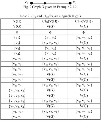
Example 2.1.2. Let G = (V(G), E(G)) be a digraph such that: V(G) = {v1, v2, v3, v4},

E(G) = {(v1, v3), (v2, v1), (v2, v3) , (v3, v4) , (v4, v1)}.

v1 v4

v2 v3

Fig. 2 Graph G given in Example 2.1.2.

Table 2: ClG and ClG2 for all subgraph H  G.

V(H) ClG(V(H)) ClG2(V(H))

V(G) V(G) V(G)

  

{v1} {v1, v3} {v1, v3, v4}

{v2} {v1, v2, v3} V(G)

{v3} {v3, v4} {v1, v3, v4}

{v4} {v1, v4} {v1, v3, v4}

{v1, v2} {v1, v2, v3} V(G)

{v1, v3} {v1, v3, v4} {v1, v3, v4} {v1, v4} {v1, v3, v4} {v1, v3, v4}

{v2, v3} V(G) V(G)

{v2, v4} V(G) V(G)

{v3, v4} {v1, v3, v4} {v1, v3, v4}

{v1, v2, v3} V(G) V(G)

{v1, v2, v4} V(G) V(G)

{v1, v3, v4} {v1, v3, v4} {v1, v3, v4}

{v2, v3, v4} V(G) V(G)

{v1, v4} {v1, v3, v4} {v1, v3, v4}

{v2, v3} V(G) V(G)

FG2 = {V(G), , {v1, v3, v4}}, TG2 = {V(G), , {v2}}.

Proposition 2.1.1. [24] Let (G, FGm) be a Gm-closure

space. If H and K are two subgraphs of G such that H

 K G, then

ClGm(V(H))  ClGm(V(K)) and IntGm(V(H)) 

IntGm(V(K)).

space. If H and K are two subgraphs of G, then (a) ClGm(V(H)  V(K)) = ClGm(V(H))  ClGm(V(K)).

(b) IntGm(V(H) ∩ V(K)) = IntGm(V(H)) ∩ IntGm(V(K)).

space. If H and K are two subgraphs of G, then

(a) ClGm(V(H) ∩ V(K))  ClGm(V(H)) ∩ ClGm(V(K)),

and

(b) IntGm(V(H))  IntGm(V(K))  IntGm(V(H) 

V(K)).

Remark 2.2.1. The converse of proposition (2.1.3) above need not be true in general, as the following example (2.3 in [24]).

Definition 2.1.3. [24] Let (G, FGm) be a Gm-closure

(3)

BdGm(V(H)) = ClGm(V(H))  IntGm(V(H)).

space and H  G, then

(a)

BdGm(V(H)) = ClGm(V(H)) ∩ ClGm(V(G)  V(P)).

(b)

BdGm(V(P)) = BdGm(V(G)  V(P)).

(c)

ClGm(V(P)) = V(P)  BdGm(V(P)).

(d)

IntGm(V(P)) = V(P)  BdGm(V(P)).

By a similar way of definitions of regular open set [27], semi-open set [16], pre-open set [18], -open set [9] (b-open set [2]), -open set [15], and -open set [1] (=semi-pre-open set [3]). We introduce the following definitions which are essential for our present study. In

Gm-closure space (G, FGm) the subgraph H in (G, FGm) is

called

(a) Regular open subgraph [24] (briefly R-osg) if V(H)

= IntGm(ClGm(V(H))).

(b) Semi-open subgraph [24] (briefly S-osg) if V(H)

 ClGm(IntGm(V(H))).

(c) Pre-open subgraph [24] (briefly P-osg) if V(H)

 IntGm(ClGm(V(H))).

(d)

-open subgraph (briefly -osg) if V(H)  ClGm(IntGm(V(H)))IntGm(ClGm(V(H))).

(e)

-open subgraph [24] (briefly -osg) if V(H)  IntGm(ClGm(IntGm(V(H))).

(f)

-open subgraph [24] (briefly -osg) if V(H)  ClGm(IntGm(ClGmV(H))).

The complement of an R-osg (resp. S-osg, P-osg,  -osg, -osg and -osg) is called R-closed subgraph (briefly R-csg) (resp. S-csg, P-csg, -csg, -csg and  -csg).

The family of all R-osgs (resp. S-osgs, P-osgs, -osgs,

-osgs and -osgs) of (G, FGm) is denoted by ROGm(G)

(resp. SOGm(G), POGm(G), OGm(G), OGm(G) and OGm(G) ). All of SOGm(G), POGm(G), OGm(G), OGm(G) and OGm(G) are larger than TGm and closed

under forming arbitrary union.

The family of all R-csgs (resp. S-csgs, P-csgs, -csgs,

-csgs and -csgs) of (G, FGm) is denoted by RCGm(G)

(resp. SCGm(G), PCGm(G), CGm(G), CGm(G) and CGm(G) ).

The near closure (resp. near interior and near boundary)of a subgraph H of G in a Gm-closure space

(G, FGm) is denoted by ClGmj (V(H)) (resp.

Int_Gmj (V(H)) and Bd_Gmj (V(H)) ) and defined by

Cl_Gmj (V(H)) = ∩{V(F) ; V(F) is j-csg and V(H) 

V(F)}.

(resp. Int_Gmj (V(H)) = V(G)  Cl_Gmj (V(G)  V(H)) and

Bd_Gmj (V(H)) = Cl_Gmj (V(H))  Int_Gmj (V(H)) ) where

j{R, S, P, , α, }.

Proposition 2.1.5. [24] Let (G, FGm) be Gm-closure

space, the implication TGm and the families of near open

and near closed graphs are given by following statements.

(a)ROGm(G)  TGm  OGm(G)  SOGm(G)  OGm(G) OGm(G),

(b)OGm(G)  POGm(G) OGm(G),

(c)RCGm(G) FGmCGm(G)  SCGm(G) CGm(G) CGm(G),

(d)CGm(G)  PCGm(G) CGm(G).

2.2. Fundamental Notions of Uncertainty

Motivation for rough set theory has come from the need to represent subsets of a universe in terms of equivalence classes of a partition of that universe. The partition characterizes a topological space, called approximation space K = (X, R), where X is a set called the universe and R is an equivalence relation [17, 21]. The equivalence classes of R are also known as the granules, elementary sets or blocks, we shall use Rx X to denote the equivalence class containing x 

X. In the approximation space, we consider two operators, the upper and lower approximations of subsets: Let A  X, then the lower approximation (resp. the upper approximation) of A is given by

L(A) = {x  X : Rx A}

(resp. U(A) = {x  X : Rx∩ A })

Boundary, positive and negative regions are also defined:

BdR(A) = U(A) – L(A),

POSR(A) = L(A),

NEGR(A) = X – U(A).

These notions can be also expressed by rough membership functions [21], namely,

X x , R

A R ) x (

x x R

A 

 

 .

Different values defines boundary (0 < R_A(x) < 1),

positive (R_A(x) = 1) and negative (R_A(x) = 0) regions.

(4)

Fuzzy set [29] is a way to represent populations that the set theory cannot describe definitely, fuzzy sets use a many (usually infinite) valued membership function, unlike classical set theory which uses a two valued membership function (i.e. an element is either in a set or it is not). Let X denotes a universal set and A  X. Then a membership function on X, A, is a function;

A : X  L for some partially order set L. L usually is a lattice [11]. Intuitively the membership function, A, gives the degree to which an element x  X is in the fuzzy set A. In the case L is the closed interval [0, 1], we call it the Standard Fuzzy Set Theory.

2. Near Rough and Near Exact Subgraphs

in G

m

-closure Spaces

The present section is devoted to introduce the near exactness and near roughness by applying the concepts of near open subgraphs to make more accuracy for definability of graphs. Let H be a subgraph of a graph G. Let IntGm(V(H)), ClGm(V(H)) and BdGm(V(H)) be

Gm-closure, Gm-interior and Gm-boundary region

respectively. H is Gm-exact if BdGm(V(H)) = 

otherwise H is Gm-rough [14]. We shall express near

Gm-rough graph properties in terms of Gm-topological

closure concepts. Let Cl_Gmj (V(H)), Int_Gmj (V(H)) and

Bd_Gmj (V(H)) be near Gm-closure, near Gm-interior, and

near Gm-boundary vertices respectively, where j{R,

S, P, , α, }. H is a near Gm-exact (briefly jGm-exact)

graph if BdGmj (V(H)) = , otherwise H is a near Gm

-rough (briefly jGm-rough). It is clear H is jGm-exact iff

Cl_Gmj (V(H)) = Int_Gmj (V(H)). In Pawlak space a subset

A  X has two possibilities rough or exact. The following definition introduces new types of near definability for a subgraph H  G in a Gm-closure

space (G, FGm).

Definition 3.1. Let (G, FGm) be a Gm-closure space and

H  G, then H is called

(a) totally jGm-definable (jGm-exact) graph if

Int_Gmj (V(H)) = V(H) = Cl_Gmj (V(H)),

(b) internally jGm-definable graph if IntGmj (V(H)) =

V(H), Cl_Gmj (V(H))  V(H),

(c) externally jGm-definable graph if IntGmj (V(H)) 

V(H), Cl_Gmj (V(H)) = V(H),

(d) jGm-indefinable (jGm-rough) graph if Int_Gmj (V(H))

 V(H), Cl_Gmj (V(H))  V(H), where j{R, S, P, , α, }.

Proposition 3.1. Let (G, FGm) be a Gm-closure space

and H be a subgraph of G. If H is Gm-exact graph, then

it is jGm-exact for all j{R, S, P, , α, }

Proof. The proofs of the six cases are similar; So, we will only prove the case when j = : Let H be Gm-exact

graph, then ClGm(V(H)) = V(H) =IntGm(V(H)). Now,

ClGm(V(H)) = ∩ {V(F) ; V(F) FGm and V(H)  V(F)}

∩{V(F) ; V(F) CGm(G) and V(H)  V(F)}

since FGm CGm(G)

= Cl_Gm (V(H)) (3.1.1)

Also, IntGm(V(H)) = V(G)  ClGm(V(G)  V(H))

 V(G)  Cl_Gm(V(G)  V(H))

since TGmOGm(G)

= Int_Gm(V(H)) (3.1.2)

From (3.1.1) and (3.1.2) we get IntGm(V(H)) 

Int_Gm(V(H))  V(H)  Cl_Gm(V(H))  ClGm(V(H)).

Since H is exist we get Int_Gm (V(H)) = V(H) =

Cl_Gm(V(H)). Hence H is Gm-exact.

The converse of the above proposition is not true in general as the following example illustrates.

Example 3.1. Let G = (V(G), E(G)) be a digraph such that: V(G) = {v1, v2, v3, v4},

E(G) = {(v2, v3), (v3, v4), (v4, v2)}.

v1. v4

v2 v3

Fig. 3 Graph G given in Example 3.1.

FG2 = {V(G), , {v1}, {v2, v3, v4}},

TG2 = {V(G), , {v1}, {v2, v3, v4}}.

Let H = (V(H), E(H)); V(H) = {v1, v2}, E(H) = . Then

IntG2(V(H)) = {v1} and ClG2(V(H)) = V(G), that is, H is

a G2-rough graph. But

Int_G₂(V(H)) = V(H) = Cl_G₂(V(H)), that is, H is G2

(5)

In a Gm-topological closure space (G, TGm), we shall

use Int_Gmj (V(H))|_TGm (resp. ClGmj (V(H))|TGm and

Bd_Gmj (V(H))|_TGm) for a subgraph H  G to denote

Int_Gmj (V(H)) (resp. Cl_Gmj (V(H)) and Bd_Gmj (V(H)) )

with respect to the Gm-topology TGm for all j{R, S, P,

, α, }.

Proposition 3.2. Let (G, FGm) and (G', F 'Gm) be two

Gm-closure space such that the family of jGm-open

subgraphs in TGm subset of the family of jGm-open

subgraphs in T 'Gm for all j{R, S, P, , α, }. If H  G,

G' is jGm-exact in (G, FGm) then H is jGm-exact in (G', F

'Gm).

Proof. Since Bd_Gmj (V(H))|T 'Gm Bd_Gmj (V(H))|TGm and

Bd_Gmj (V(H))|TGm =  for all j{R,S,P, ,α, }. Then

Bd_Gmj (V(H))|T 'Gm =  and H is jGm-exact with respect

to T 'Gm.

In Proposition (3.2), it is not necessary for TGm to be

coarser than T 'Gm, also the converse of this proposition

is not true in general as the following example illustrates.

Example 3.2. Let G = (V(G), E(G)) and G' = (V(G), E(G')) be two digraph such that V(G) = {v1, v2, v3, v4},

E(G) = {(v1, v2), (v1, v3), (v1, v4), (v2, v1), (v2, v3), (v4,

v3)} and E(G') = {(v2, v3), (v3, v4), (v4, v2)}.

v1 v4 v1 . v4

v2 v3 v2 v3

G G' Fig. 4 Graph G and G' given in Example 3.2.

FG1 = {V(G), , {v3}, {v3, v4}, {v1, v2, v3}}, TG1 = {V(G), , {v4}, {v1, v2}, {v1, v2, v4}}. F 'G2 = {V(G), , {v1}, {v2, v3, v4}}, T 'G2 = {V(G), , {v1}, {v2, v3, v4}}.

Then POG1(G)|TG1 POG2(G')|T 'G2.

If H = (V(H), E(H)); V(H)={v4}, E(H) = ,

BdGP1(V(H))|TG1 = {v3} and BdGP'2(V(H))|T 'G'2 = .

Thus H is is PG2-exact graph in T 'G'2 but it is not PG1

-exact in TG1.

Lemma 3.1. Let (G, FGm) and (G', F 'Gm) be two Gm

-closure space and H is a subgraph of G, G'. Then

Cl_Gmj (V(H))|T 'Gm = Cl_Gmj (V(H))|TGm if and only if

Int_Gmj (V(H))|T 'Gm = IntGmj (V(H))|TGm for all j{R, S,

P, , α, }.

Proof. The proofs of the six cases are similar; So, we will only prove the case when j = : Now,

Cl_Gm(V(H))|_T'Gm = ClGm(V(H))|TGm if and only if

∩ {V(F)  V(G); V(H)  V(F), V(F) CGm(G') with

respect to T 'G'}

= ∩ {V(F)  V(G); V(H)  V(F), V(F)  CGm(G)

with respect to TG}

if and only if

V(G) – ∩ {V(F)  V(G); V(H)  V(F), V(F) 

CGm(G') with respect to T 'G'}

= V(G) – ∩ {V(F)  V(G); V(H)  V(F), V(F) 

CGm(G) with respect to T G}

if and only if

{V(G)–V(F)V(G);V(G)–V(H)V(G)–V(F), V(G)–

V(F) OGm(G') w. r. t. T 'G'}

={V(G)–V(F)V(G);V(G)–V(H)V(G)–V(F),

V(G)–V(F)OGm(G) w. r. t. TG}

if and only if

Int_Gmj (V(H))|_T'Gm = Int j

Gm(V(H))|TGm.

Let us observe Lemma 3.1. The following proposition

gives the condition for jGm-exact graphs in (G', F 'Gm) to

be jGm-exact graphs in (G, FGm), where the family of

jGm-open graphs in (G, FGm) subset of the family of

jGm-open graphs in (G', F 'Gm) for all j{R,S,P, , α, }.

Proposition 3.3. Let (G, FGm) and (G', F 'Gm) be two

Gm-closure space such that the family of jGm-open

subgraphs in TGm subset of the family of jGm-open

subgraphs in T 'Gm for all j{R, S, P, , α, }. Then

(6)

Gm) if and only if Cl j

Gm(V(H))|TGm = Cl_Gmj (V(H))|T 'G'm

for all subgraph H  G, G'.

Proof. If H is jGm-exact graph in (G', F 'G'm) for all

j{R, S, P, , α, }, then Cl_Gmj (V(H))|T 'G'm = V(H) and

Cl_Gmj (V(H))|TGm = V(H), hence ClGmj (V(H))|TGm =

Cl_Gmj (V(H))|T 'G'm . Conversely, if ClGmj (V(H))|TGm =

Cl_Gmj (V(H))|_T'G'm and H is jGm-exact in (G', F 'G'm).

Then H is jGm-exact in (G, FGm).

3. Near Rough Membership Function in

G

m

-closure Spaces

Original rough membership function is defined using equivalence classes. It was extended to topological

spaces [15], namely. If TGm is a Gm-topology on a finite

graph G, then the Gm-rough membership function for

subgraph H on G is

H

Gm(v) =

| } ) K ( V { | | )) H ( V )} K ( V { | v v   

, v  G (4.1)

where Kv is any suggraph of TGm containing v.

In equation (4.1), since it is not necessary for { ∩ Kv }

to be a j-open graph for all j{R, S, P, , α, }, then we cannot use this equation to express j-boundary region, j-interior and j-exterior of a subgraph H  G in a Gm

-closure space (G, FGm) even thought Kv is a j-open

graph.

Example 4.1. Let (G, FGm) be a Gm-closure space

which is given in Example (2.1.1).

FG1 = {V(G), , {v3}, {v3, v4}, {v1, v2, v3}}, TG1 = {V(G), , {v4}, {v1, v2}, {v1, v2, v4}},

OG1(G) = {V(G),  {v1}, {v2}, {v4}, {v1, v2}, {v1, v3}

{v1, v4}, {v2, v3}, {v2, v4}, {v3, v4}, {v1, v2, v3}, {v1, v2,

v4}, {v1, v3, v4}, {v2, v3, v4}}.

If H = (V(H), E(H)); V(H)={v1, v3, v4}, E(H)= {(v1,

v3), (v4, v3)}, in equation (4.1), then

H

Gm(v1) =

| } ) K ( V { | | } v , v , v { )} K ( V { | 1 1 v 4 3 1 v    2 1 | } v , v { | | } v , v , v { } v , v { | 2 1 4 3 1 2 1 _   ,

That is v1IntGm(V(H)); but IntGm(V(H)) = {v1, v3,

v4}.

Also, in the case of Kv OGm(G) and H = (V(H),

E(H)); V(H) = {v3}, E(H) = , then

H

Gm(v3) = 1

| } v { | | } v { } v { | | } ) K ( V { | | } v { )} K ( V { | 3 3 3 v 3 v 3

3   

  

; but

Int_Gm(V(H)) = .

In a Gm-closure space (G, FGm), we use jGm-boundary

region "briefly jBdGm(V(H))" (resp. jGm-positive region

"briefly jPOSGm(V(H))" and jGm-negative region

"briefly jNEGGm(V(H))) to denote Bd_Gmj (V(H)) (resp.

Int_Gmj (V(H)) and Ext_Gmj (V(H)) ) for a subgraph H 

G, where j{R, S, P, , α, }.

we introduce the following definition for a jGm-rough

membership function to express jBdGm (V(H)),

jPOSGm(V(H))) and jNEGGm(V(H))) for a subgraph H 

G, where j{R, S, P, , α, }.

H  G. Then the near Gm-rough (briefly jGm-rough)

membership function on G is jH_Gm : G  [0, 1] and it

is given by

jH Gm(v) =

         otherwise )) H ( V ( K min )), H ( V ( K 1 if 1 v j v j

where jKv(V(H)) =

       opengraph,v V(K) Gm a is K : | ) K ( V | | ) H ( V ) K ( V | j 

for all j{R, S, P, , α, }.

Theorem 4.1. Let (G, FGm) be a Gm-closure space and

H  G. Then

(a) v  Int_Gmj (V(H)) if and only if jHGm(v) = 1,

(b) v  Bd_Gmj (V(H)) if and only if 0 < jH_Gm(v) < 1,

(c) v  is a jGm-exterior vertex of H (briefly v 

EXT_Gmj (V(H)) ) if and only if jH_Gm(v) = 0.

For all j{R, S, P, , α, }.

Proof. The proofs of the six cases are similar; So, we will only prove the case when j = :

(a) v  Int_Gm(V(H)) iff  K OGm(G) such that v 

V(K)  V(H)

iff  K  OGm(G), v  V(K) such that

| ) K ( V | | ) H ( V ) K ( V |  = 1

(7)

(b) v  Bd_Gm(V(H)) iff  K OGm(G), v  V(K),

we have V(K) ∩ V(H)   and V(K) ∩ (V(G) – V(H)) 

iff  K OGm(G), v  V(K), we have 0 < | V(K)

∩ V(H) | < | V(K) |

iff  K  OGm(G), v  V(K), we have 0 <

| ) K ( V |

| ) H ( V ) K ( V

| 

< 1

iff 0 < jH_Gm(v) < 1.

(c) v  EXT_Gm(V(H)) iff  K OGm(G) such that v  V(K)  (V(G) – V(H))

iff  K OGm(G), v  V(K) such that V(K) ∩

V(H) = 

iff  K  OGm(G), v  V(K) such that

| ) K ( V |

| ) H ( V ) K ( V

| 

= 0

iff HGm(v) = 0.

The jGm-rough membership function defines

jBdGm(V(H)) (resp. jPOSGm(V(H)) and jNEGGm(V(H))

if 0 < jHGm(v) < 1 (resp. jHGm(v) = 1 and jHGm(v) =

0) for all j{R, S, P, , α, } in a Gm-closure space (G, FGm) and H  G. The following example illustrates

Theorem (4.1) for j{ , α, }.

FG1 = {V(G), , {v3}, {v3, v4}, {v1, v2, v3}}, TG1 = {V(G), , {v4}, {v1, v2}, {v1, v2, v4}},

OG1(G) = {V(G), , {v1}, {v2}, {v4}, {v1, v2}, {v1, v4},

{v2, v4}, {v3, v4}, {v1, v2, v3}, {v1, v2, v4}, {v1, v3, v4},

{v2, v3, v4}},

OG1(G) = {V(G), , {v4}, {v1, v2}, {v1, v2, v4}}, and OG1(G) = {V(G), , {v1}, {v2}, {v4}, {v1, v2}, {v1,

v3} {v1, v4}, {v2, v3}, {v2, v4}, {v3, v4}, {v1, v2, v3},

{v1, v2, v4}, {v1, v3, v4}, {v2, v3, v4}}.

If H = (V(H), E(H)); V(H)={v1, v3}, E(H)= {(v1, v3)},

we get:

GmH (v1) = 1/3, GmH (v2) = 1/3,HGm(v3) = 1/2,

GmH (v4) = 0,

GmH (v1) = 1, GmH (v2) = 0, HGm(v3) = 1/3,

GmH (v4) = 0,

HGm(v1) = 1, HGm(v2) = 0, HGm(v3) = 1, GmH (v4)

= 0, Therefore

Int_Gm(V(H)) = {v1}, Bd_Gm(V(H)) = {v3},

EXT_Gm(V(H)) = {v2, v4},

Int_Gm(V(H)) = , Bd_Gm(V(H)) = {v1, v2, v3},

EXT_Gm(V(H)) = {v4},

Int_Gm(V(H)) = {v1, v3}, BdGm(V(H)) = , EXT



Gm

(V(H)) = {v2, v4}.

4. Near Fuzzy Graphs in G

m

-closure

spaces

Near membership functions allow us to express fuzzy theory in Gm-closure spaces. In the following definition

we define a near Gm-fuzzy (briefly jGm-fuzzy) graph by

using the jGm-rough membership function of Gm

-closure spaces for all j{R, S, P, , α, }.

H  G. The jGm-fuzzy graph of H is denoted by jHf and

is given by

jH f

= {(v, jH_Gm(v)) : for all v  G }, j{R,S,P, ,α, }.

then

Hf = {(v1, 1), (v2, 0), (v3, 1/3), (v4, 0)},

Hf = {(v1, 1/3), (v2, 1/3), (v3, 1/2), (v4, 0)}, and

Hf = {(v1, 1), (v2, 0), (v3, 1), (v4, 0)}.

Now, we introduce some simple operations on jGm

-fuzzy graphs for all j{R, S, P, , α, }.

Definition 5.2. Let H and K be two subgraphs of G in a Gm-closure space (G, FGm). We say that jHf is included

in jKf (briefly jHf jKf) for all j{R, S, P, , α, } if

and only if

jH

Gm(v)  jKGm(v) for all v  G.

Definition 5.3. Let H and K be two subgraphs of G in a Gm-closure space (G, FGm). We say that jH

f

and jK f

are

equal (briefly jHf = jKf) for all j{R, S, P, , α, } if

and only if

jH

Gm(v) = j K

Gm(v) for all v  G.

If at least one v of G is such that the equality jHGm(v)

= j_GmK (v) is not satisfied, we say that jH f

and jK f

are

(8)

Definition 5.4. Let H and K be two subgraphs of G in a Gm-closure space (G, FGm). We say that jH

f

and jK f

are

complementary (briefly jK f

= jH fc

) for all j{R, S, P, , α, } if and only if

jK

Gm(v) = 1 – j H

Gm(v) for all v  G.

One obviously has (jH fc

)c = jH f

for all j{R,S,P, ,α, }.

then

Hf = {(v1, 1), (v2, 0), (v3, 1/3), (v4, 0)},

Hfc = {(v1, 0), (v2, 1), (v3, 2/3), (v4, 1)}.

Definition 5.5. Let H, K and M be subgraphs of G in a Gm-closure space (G, FGm). We define the intersection

jHf∩jKf for all j{R, S, P, , α, } as the largest jGm

-fuzzy graph contained at the same time in jHf and jKf.

that is, if jM f

= jH f_∩

jK f

, then

jM

Gm(v) = min { j H Gm(v), j

K

Gm(v) } for all v  G.

Definition 5.6. Let H, K and M be subgraphs of G in a Gm-closure space (G, FGm). We define the union jH

f_

jK f

for all j{R, S, P, , α, } as the smallest jGm-fuzzy

graph contains both jH f

and jK f

. that is, if jM f

= jH f_

jK f

, then

jM

Gm(v) = max { j H Gm(v), j

K

Gm(v) } for all v  G.

If H = (V(H), E(H)); V(H) ={v1, v3}, E(H) = {(v1, v3)},

and If K = (V(K), E(K)); V(K) = {v1, v2, v3}, E(H) =

{(v1, v2), (v1, v3), (v2, v1), (v2, v3)}, then

v1 v1

v2 v3 v3

H K

Fig. 5 Subgraph H and K given in Example 5.3.

Hf = {(v1, 1/3), (v2, 1/3), (v3, 1/2), (v4, 0)},

Kf = {(v1, 1), (v2, 1), (v3, 3/4), (v4, 0)},

Hf∩Kf = {(v1, 1/3), (v2, 1/3), (v3, 1/2), (v4, 0)},

HfKf = {(v1, 1), (v2, 1), (v3, 3/4), (v4, 0)}.

Definition 5.7. Let H and K be two subgraphs of G in a Gm-closure space (G, FGm). The disjunction sum of two

jGm-fuzzy graph for all j{R, S, P, , α, } is define in

terms of union and intersections in the following fashion

jHfjKf = (jHf∩jKfc)  (jHfc∩jKf).

Example 5.3. In Example (4.3)., we get

Hf = {(v1, 1/3), (v2, 1/3), (v3, 1/2), (v4, 0)},

Kf = {(v1, 1), (v2, 1), (v3, 3/4), (v4, 0)}. Hence

Hfc = {(v1, 2/3), (v2, 2/3), (v3, 1/2), (v4, 1)},

Kfc = {(v1, 0), (v2, 0), (v3, 1/4), (v4, 1)},

Hf∩Kfc= {(v1, 0), (v2, 0), (v3, 1/4), (v4, 0)},

Hfc ∩ Kf= {(v1, 2/3), (v2, 2/3), (v3, 1/2), (v4, 0)}.

Thus

HfKf = (Hf∩Kfc)  (Hfc∩Kf) = {(v1, 2/3),

(v2, 2/3), (v3, 1/2), (v4, 0)}.

Definition 5.8. Let H and K be two subgraphs of G in a Gm-closure space (G, FGm). The difference jH

f

– jK f

for

all j{R, S, P, , α, } is define by

jH f

– jK f

= jH f_∩

jK fc

.

Of course, except in particular cases, jHf – jKf = jKf –

jHf for all j{R, S, P, , α, }.

Hf = {(v1, 1/3), (v2, 1/3), (v3, 1/2), (v4, 0)},

Kf = {(v1, 1), (v2, 1), (v3, 3/4), (v4, 0)}. Then

Hf –Kf = Hf∩Kfc= {(v1, 0), (v2, 0), (v3, 1/4), (v4,

0)}, since

Kfc= {(v1, 0), (v2, 0), (v3, 1/4), (v4, 1)}.

Definition 5.9. Let H and K be two subgraphs of G in a finite Gm-closure space (G, FGm). The j-Hamming

distance between H and K for all j{R, S, P, , α, } is define by

jd(H, K) =





   n

1 i

i K Gm j i H Gm

j (v) (v)|

| .

Hf = {(v1, 1/3), (v2, 1/3), (v3, 1/2), (v4, 0)}, and

Kf = {(v1, 1), (v2, 1), (v3, 3/4), (v4, 0)}. Then

d(H, K) = | 1/3 – 1 | + | 1/3 – 1 | +| 1/2 – 3/4 | +| 0 – 0 |

= 2/3 + 2/3 + 1/4 +0 = 1.583 .

Definition 5.10. Let H and K be two subgraphs of G in a finite Gm-closure space (G, FGm). The j-Euclidean

(9)

je(H, K) =



    n 1 i 2 i K Gm j i H Gm

j (v) (v))

( .

Definition 5.11. Let H and K be two subgraphs of G in a finite Gm-closure space (G, FGm). The j-Euclidean

norm between H and K for all j{R, S, P, , α, } is define by

je 2

(H, K) =



   n 1 i 2 i K Gm j i H Gm

j (v) (v))

( .

Hf = {(v1, 1/3), (v2, 1/3), (v3, 1/2), (v4, 0)}, and

Kf = {(v1, 1), (v2, 1), (v3, 3/4), (v4, 0)}. Then

je(H, K) = 4/94/91/160 0.9510.975, and

je 2

(H, K) = 4/9 +4/9 +1/16 +0 = 0.951.

Definition 5.12. Let H and K be two subgraphs of G in a finite Gm-closure space (G, FGm). The generalized

relative j-Euclidean between H and K for all j{R, S, P, , α, } is define by

j(H, K) = n ) K , H ( d j =



    n 1 i i K Gm j i H Gm

j (v) (v)|

| n 1

.

Hf = {(v1, 1/3), (v2, 1/3), (v3, 1/2), (v4, 0)}, and

Kf = {(v1, 1), (v2, 1), (v3, 3/4), (v4, 0)}. Then

(H, K) =

4 583 . 1

= 0.396 .

Definition 5.13. Let H and K be two subgraphs of G in a finite Gm-closure space (G, FGm). The relative

j-Euclidean between H and K for all j{R, S, P, , α, } is define by

j(H, K) =

n ) K , H ( e j =



    n 1 i 2 i K Gm j i H Gm

j (v) (v))

( n 1

.

Definition 5.14. Let H and K be two subgraphs of G in a finite Gm-closure space (G, FGm). The relative

j-Euclidean norm between H and K for all j{R, S, P, , α, } is define by

j2_{(H, K) =}

n ) K , H ( e2 j =



    n 1 i 2 i K Gm j i H Gm

j (v) (v))

( n 1

.

Hf = {(v1, 1/3), (v2, 1/3), (v3, 1/2), (v4, 0)}, and

Kf = {(v1, 1), (v2, 1), (v3, 3/4), (v4, 0)}. Then

(H, K) = 2 975 . 0

= 0.488 , and

2(H, K) =

4 ) 975 . 0 ( 2

= 0.238 .

6. Conclusions

In this paper, we used Gm-closure space concepts to

introduce definitions to near rough, near exact and near fuzzy graphs. We generalize near rough graphs in the frameworks of topological spaces. We believe such generalization will be useful in digital topology [22] as well as biomathematics [26]. The topological applications which introduced help for measuring near exactness and near roughness of graphs. Our approach is to topologize information systems. We connect near rough graphs, topological spaces, near rough membership function, and near fuzzy graphs.

References

[1] M. E. Abd El-Monsef, S. N. El-Deeb, R. A. Mohmoud, -open sets, -continuous mappings, Bull. Fac. Sc. Assuit Univ., 12(1983), 77-90. [2] D. Andrijevic, On b-open sets, Mat. Vesnik, 48

(1996),59-64.

[3] D. Andrijevic, Semi-preopen sets, ibid. 38(1986), 24-32.

[4] R. Belohlavek, Fuzzy Closure Operators, J. of math. Analysis and Application, 262 (2001), 473-491.

[5] G. Birkhoff, Lattice Theory, AMS Colloq Publications, Providence, 6 RI, 1940, (3 rd edition, 1967).

(10)

[7] W. Buszkowski, A representation Theorem for Co-diangonalizable Al-gebras, Reports on Mathematical Logic, 38 (2004),13-22.

[8] D. Dikranjan, W. Tholen, Catergorical Structure of Closure Operators, Klumer Academic Publishers, Dordrecht, 1995.

[9] A. A. El-Atik, A study of Some Types of Mappings on Topological Spaces, M. Sc. Thesis, Tanta Univ. (1997).

[10] G. Elsalamony, On Two Types of Fuzzy Closed Sets, J. Egypt. Math. Soc. Vol.15(1) (2007) pp.69-78.

[11] A. Galton, A generalized Topological View of Motion in Discrete Space, Theory. Comput. Sci. (2002).

[12] M. Goldstern, Lattices, Interpolation and set Theory, In Contr. General Algebra 12 (2000), 23-36.

[13] C. Kuratowski, Topolgie, Warsaw,1952.

[14] C. Largeron, S. Bonneray, A pre-topological Approach For Structural Analysis, Information Scienecs, 144, (2002), 169-185.

[15] E. Lashin, A. Kozae, A. Abo Khardra and T. Medhat, Rough Set Theory for Topological spaces, International Journal of Approximate Reasoning 40 (2005) 35-43.

[16] N. Levine, Semi-open Sets and Semi-continuity in Topological Spaces, Amer Math. Monthly, 70 (1963), 36-41.

[17] T.Y. Lin, Topological and Fuzzy Rough Sets, in: R. Slowinski (Ed.), Decision Supportby Experience-Application of the Rough Sets Theory, Kluwer Academic Publishers, 1992, pp. 287–304. [18] A. S. Mashhour, M. E. Abd Monsef, S. N.

El-Deeb, On pre continuous and weak pre continuous mappings, Proc. Math. Phys. Soc. Egypt, 53 (1982), 47-53.

[19] O. Njastad, On Some Classes of Nearly Open Sets, Pacific J. Math., 15(1956), 961-970.

[20] Z. Pawlak, Rough Sets, Int. J. Information Comput. Sci. 11(5) (1982) 341-356.

[21] Z. Pawlak, Rough Sets, Theoretical Aspects of Reasoning about Data, Kluwer Academic, Boston, 1991.

[22] A. Rosenfeld, Digital Topology, American Mathematical Monthly 86 (1979), 621-630.

[23] W. Shi, K. Liu, A fuzzy Topology for Computing the Interior, Boundary, and Exterior of Spatial Objects Quantitatively in GIS, Computer & Geosciences, 33 (2007), 898-915.

[24] M. Shokry, Y. Y. Yousif, Closure Operators on Graphs, Australian J. of Basic and Applied Sciences (preprint 2011).

[25] M. Shokry, Y. Y. Yousif, Connectedness in Graphs and Gm-closure spaces. Int. J. Math. &

Computer Sciences, Vol.22 No.3 (preprint 2011). [26] B.M.R. Stadler, P.F. Stadler, Generalized

Topological Spaces in Evolutionary Theory and

Combina-torial Chemistry, J.Chem.Inf.Comput.Sci.42(2002) 577-585.

[27] M. Stone, Application of the Theory of Boolian Rings to General Topology, Trans. Amer, Math. Soc., 41(1937), 374-481.

[28] W-Z Wu, W-X Zharg, Constructive and Axiomatic Approaches of Fuzzy Approximation Operators, Information Sciences, 159 (2004), 233-254.

[29] L. A. Zadeh, Fuzzy Sets, Information and Control 8 (1965) 338-352.

A. R. Radwan, PhD. He was born in Cairo, Egypt in 1958. He received the PhD in pure Mathematics from Ain Shams University in 1991. He received the M. Sc. in pure Mathematics from Ain Shams University, Faculty of Science, Department of Mathematics in 1986. Moreover, he is currently Professor and head of Department of Mathematics, Faculty of Science, Ain Shams University, Cairo-Egypt.

Y. Y. Yousif. is Ph.D student in pure Mathematics (New studies for topological generalizations and uncertainty in graph theory) in department of Mathematics, Faculty of Science, Ain Shams University, Cairo-Egypt. He was born in Baghdad, Iraq in 1971. He completed his M.Sc in Mathematics Science, Faculty of Graduate Study, University of Jordan, Amman, 2001. He is a permanent lecturer in department of Mathematics, Faculty of Education Ibn-Al-Haitham, Baghdad University, Baghdad-Iraq.