Blenders for a non-normally Hénon-like family.

UNIVERSIDADE FEDERAL DE MINAS GERAIS

INSTITUTO DE CI ˆ

ENCIAS EXATAS - ICEX

DEPARTAMENTO DE MATEM ´

ATICA

Jailton Viana da Concei¸c˜ao Advisor: Mario Jorge Dias Carneiro

Blenders For a Non-Normally H´

enon-Like Family

JULY/2012

1 Introduction 1

2 Background 2

3 Blender in 3D 7

4 Examples of Blenders 12

4.1 The Affine Blender . . . 12 4.2 Blender in the Henon-Like Family . . . 17

Bibliographics References 37

Chapter 1

Introduction

Consider the familyψ((a, b),(x, y,)) = (1₋ax2_{+by, x). We know by Benedicks- Calerson (see [4]) that this} two dimensional family have some strange atractor(see[15] for definition) for some parameters values a and b

and we also kow that inside this atractor we have a homoclinic tangence (see [12] ).

This work is a detailed study of [1] where is considered the familyϕ:R4_×R3 _→R3_{given byϕ((a, b, c, d),(x, y, z)) =} (1−ax2_{+by, x, cz+dx).}

This is a 3-dimensional version of the Henon family called in [1] Non-Normally Henon Like family. It is proved that if the parameters satisfy _

     

0<_|b_|< δ;

a > 15(1+₄|b|)2; _P._C

1 +_|d_|< c < 10₉; 0<|d|< 1₉.

then this family have a blender (we are going to define Blender late). This object was used in [10] to obtain robust heterodimensional cycle and in [2] to obtain non-uniformly hyperbolic robustly transitive diffeomorphism.

Background

Now we are going to present some definitions and results about hyperbolic dynamics. We will not prove no result here but the reader can find a proof in [5, 14].

Definition 2.0.1 Let M _{be a C}k_{-manifold and let f ∈C}1_{(M,M). One say that a point x∈ M is a hyperbolic}

fix point of f when the spectrum of the linear function df(p) : TxM → TpM has no intersection with the circle

S1 _{⊂C. One say that a point p∈M is periodic hyperbolic point(with period k) of f when it is a hyperbolic fix}

point of fk_.

Definition 2.0.2 Let M _{be a metric space and let f ∈C}0₍M_,M_{) and x∈}M_. • One call stable set of a point x the set Ws_{:={y∈M| lim}

n→∞Dist(fn(y), fn(x)) = 0}

If f ∈Homeom(M_,M_{) then}

• One call unstable set of xthe set Wu _{:={y∈M| lim}

n_→∞Dist(f−n(y), f−n(x)) = 0}, that is, the unstable

set of x is the stable set ofx by f−1_;

• One call local stable set of x(with sizeǫ >0) the set Ws

ǫ(x) :={y∈M| Dist(fn(y), fn(x))< ǫ, ∀n ≥0};

• One call local unstable set of x (with size ǫ > 0) the set Wu

ǫ (x) := {y ∈ M| Dist(f−n(y), f−n(x)) <

ǫ, _∀n_≥0_};

Theorem 2.0.1 (The Hartman₋Grobman Theorem)

Let M _{be a C}k_{-manifold and letf ∈Dif f}1_{(M)with a hyperbolic fix point p∈M. Then there are neighborhoods}

Vp ⊂M and V0 ⊂TpM and a h∈Homeom(Vp, V0) such that

h_◦f =df(p)_◦h.

Corollary 2.0.1 Let M _{be a C}k_{-manifold, f ∈C}0_{(M,M) and p∈M a hyperbolic fix point of f. Then there is}

ǫ0 >0 such that: • Ws

ǫ0(p)⊂W

s_{(p) and W}u

ǫ0(p)⊂W

u_(p);

• Ws

ǫ0(p) is a topological sub-manifold with the same dimension of E

s_(p);

• Wu

ǫ0(p) is a topological sub-manifold with the same dimension of E

u_(p);

3

Figure 2.1: λ-Lemma

• Ws_{(p) =}S

n_≤0f−n(Wǫs0(p)) and W

u_{(p) =}S

n_≤0fn(Wǫu0(p)) are immersed topological sub-manifolds

Proof: It follows immediately from the Hartman-Grobman Theorem.

Corollary 2.0.2 Suppose p is a hyperbolic fix point of f thus there is a neighborhood Vp ⊂ M such that if

fn_(q)∈V

p for all n ∈Z then q=p.

Lemma 2.0.1 (The λ₋Lemma)

Suppose that

• M _{is a connected compact boundaryless C}r_{- Riemannian manifold of dimension n;} • f ∈Dif fr_(M);

• p_∈M _{is a periodic hyperbolic point for f;} • Du _{is a compact disc in W}u_(p);

• D is a disc centered in a point x_∈Ws_{(p) such that dim(D) = dim(W}u_{(p)) and x∈D⋔W}s_(p).

Then for every ε > 0 there is an integer n0 > 0 such that for all n ≥ n0 there is a disc Dn ⊂ D so that

fn_(D

n) is a disc ε−C1-near of Du.

Definition 2.0.3 (Hyperbolic set)

1. Λ compact invariant ;

2. For every x∈Λ there is subspaces Es_{(x), E}u_(x)⊂T

xM such that:

(a) TxM=Es(x)⊕Eu(x);

(b) df(x)(Es_{(x)) =E}s_{(f(x)) and df(x)(E}u_{(x)) =E}u_(f(x));

(c) There are constants c > 0 and 0< λ < 1 such that: i. kdfn_{(x)(v)k ≤cλ}n_{kvk, ∀v ∈E}s_{(x) and ∀n≥0;}

ii. _kdf−n_(x)(v)

k ≤cλn

kv_k, _∀v _∈Eu_{(x) and}

∀n _≥0. The sub-bundles Es _:=

∪x∈Λ{(x, v)|x ∈Λ and v ∈Es(x)} and Eu :=∪x∈Λ{(x, v)|x∈Λ and v ∈Eu(x)}

are called stable sub-bundle and unstable sub-bundle respectively and we have TΛM=Es⊕Eu.

On this way if p is a hyperbolic periodic point of f with period k, then Λ = _{p, f(p), f2_{(p), ...., f}k−1_{(p)} is a}

hyperbolic set for f. Note that hyperbolicity does not depends on the Riemannian Metric.

Proposition 2.0.1 If f ∈Dif fr_{(M) and Λ ∈M is a hyperbolic set for f then the subspaces E}s_{(x) and E}u_(x)

depends continuously on the point x.In particular , they have dimensions locally constant.

Proposition 2.0.2 (Adapted Meric) If f _∈ Dif fr_{(M) and Λ}

⊂ M _{is a hyperbolic set for f, then there is a}

C∞_{- Riemannian Metric on} M _{and a constant 0< a <1 such that:} • kdf(x)(vs_{)k∗ < akv}s_{k∗, ∀v}s_∈Es_{(x) and ∀x∈Λ;}

• kdf−1_(x)(vu_{)k∗ < akv}u_{k∗, ∀v}u _∈Eu_{(x) and ∀x∈Λ;}

Where _k._k∗ is the norm which come from the metric.

Definition 2.0.4 Let V a real Hilbert space. We say that a set C _⊂V is a cone on V if and only if ,V admits a splitting V =E⊕F and there is a real number a >0 such that

C=_{(vE, vF)∈V| kvEk ≤akvFk}

Proposition 2.0.3 Let V be a real Hilbert space. Then a set C _⊂V is a cone on V if, and only if, there is a continuous non-degenerated quadratic form B :V →R _{such that}

C =_{v _∈V_| B(v)_≤0_}.

Definition 2.0.5 Let V be a Hilbert space with finite dimension and let C be a cone on V.

• We say that the cone C has dimension k when k =M ax{dimW| W ⊂C is a subspace of V}.

• We say that a non-degenerated quadratic form B : V → R _{has dimension k if k is the dimension of the}

cone determined of it.

5

• One call a continuous field of quadratic form a functionB which associates to each pointx∈Λ a quadratic form B(x) : TxM → R. By continuous one means that the coefficients of the quadratic forms B(x) are

continuous real functions on Λ.

• One call a continuous cone-field on Λ a function C which to each point x _∈Λ associates a cone C(x) in

TxM. By continuous cone-field one means that the field of quadratic form determined byC is a continuous

field of quadratic form.

• If f _∈C1_{(M,M) and B is a continuous field of quadratic form on Λ, one call the pull-back of B the field}

of quadratic form defined by

(f∗B)(x) = B(f(x))(df(x)(v))

where we are supposing that f(Λ)_⊂Λ.

Theorem 2.0.2 (Characterization of hyperbolicity via cone₋fields)

Suppose that

• M _{is a connected compact boundaryless C}r_{- Riemannian manifold of dimension n;} • f _∈Dif fr_(M);

• Λ ⊂M _{is compact f-invariant.}

The following statements are equivalent : 1. Λ is a hyperbolic set for f;

2. There is a continuous field B of non-degenerated quadratic forms on Λ and whose dimension is constant through the orbits of f in points of Λ and such that the quadratic form f∗_{B−B is positive defined, where}

f∗_{B(v) = B(f(v)).}

3. There is on Λ ,two continuous cone-fields Cs _{and C}u _{where the dimensions of them are point-wise}

com-plements and constant through the orbits of f in points of Λ and such that : (a) df(x)(Cu_(x))⊂Cu_{(f(x)) and df−}1_(x)(Cs_(x))⊂Cs_(f−1_(x));

(b) There is σ > 1 and m >0 such that

i. kdfm_{(x)(v)k ≤σkvk , ∀v ∈C}u_{(x) and ∀x∈Λ;}

ii. kdf−m_{(x)(v)k ≤σkvk , ∀v ∈C}s_{(x) and ∀x∈Λ.}

Theorem 2.0.3 (The Stable Manifold Theorem)

Suppose that

• M _{is a connected compact boundaryless C}r_{- Riemannian manifold of dimension n;}

• f ∈Dif fr_(M);

• Λ _⊂M _{is a hyperbolic set forf.}

• Ws

ε(x) is a Cr-Embedded sub-manifold of M so that TxWεs(x) = Es(x);

• Ws

ε(x)⊂Ws(x);

• Ws_{(x) =} S

n_≤0f−n(Wεs(fn(x))) and is a Cr-Immersed sub-manifold of M. Moreover Ws(x) depends

continuously on the point x.

Obviously there is an analogously result for Wu_{(x) because W}u_{(x, f) = W}s_{(x, f−}1_).

Corollary 2.0.3 In the same hypothesis of the previous theorem one can deduce that there is δ >0 such that for every x, y _∈Λ with d(x, y)< δ one have Ws

Chapter 3

Blender in 3D

In this chapter following [2] we are going to define blender and prove some properties of such object.

Rougly speaking a Blender is a hyperbolic set Λ, locally maximal invariant with a dense orbit such that Ws_(Λ)

is locally homeomorphic to the product of a Cantor set by an interval. But it bahaves as a topological surface in the following sense: There is a conefield _Cuu _{around the strong unstable direction of Λ so that every curve}

γ tangent to Cuu _{intersects W}s_{(Λ)(see lemma 3.0.6). That is why we need of the hyperbolicity theory in the}

background.

So here is the definition of Blender.

Definition 3.0.7 Let M3 _{be a boundaryless Riemaniann manifold of dimension 3 and f ∈ Dif f}1₍M3_).

Con-sider the box

B_{:= [−1,1]×[−1,1]×[−1,1]⊂}R3 _and D _{the image of an embedding E :O ⊃}B_→M3_.

Decompose the boundary of D _{into three parts as follow:}

∂uu_D=

E((_{−1_{} ∪ {}+1_})_×[₋1,1]_×[₋1,1])

∂u_D=

E([₋1,1]_×[₋1,1]_×(_{−1_{} ∪ {}+1_}))

∂sD_{=E([−1,1]×({−1} ∪ {+1})×[−1,1])}

Suppose that :

• There is a connected component A _of D_∩f(D_{) disjoint from the union ∂}sD_∪f(∂uD_);

• There are an integer n0 >0 and a connected component B of fn0(D)∩D so that B is disjoint from ∂sD,

from f(∂uu_{D) and from E([−1,1]×[−1,1]× {+1}). (See Figure)}

• There is a cone field Cu_{(q) on f−}1_(A)∪f−n0

(B_{) such that :}

– _∀q_∈f−1_{(A)⇒df(q)(C}u_(q))⊂Int(Cu_(f(q)));

– _∀q_∈f−n0(_B)

⇒dfn0(q)(Cu(q))

⊂Int(Cu_(fn0(q))).

• There is a cone field Cuu_(q)⊂Cu_{(q) on f}−1_(A)∪f−n0(_B) such that :

– _∀q∈f−1_{(A)⇒df(q)(C}uu_(q))⊂Int(Cuu_(f(q)));

– _∀q∈f−n0

(B_)⇒dfn0

(q)(Cuu_(q))⊂Int(Cuu_(fn0 (q))).

• There is a cone field Cs_{(q) on A∪B such that :}

– _∀q∈A_⇒df−1_(q)(Cs_(q))⊂Int(Cs_(f−1_(q)));

– _∀q_∈B_⇒df−n0(q)(Cs(q))

⊂Int(Cs_(f−n0(q))).

Then we have the followings definitions:

• We say that a segment L of smooth curve in D _{is an unstable segment when L is tangent to C}uu _{and its}

boundary ∂L is contained in ∂uu_{D. We shall denote an unstable segment for L}u_.

• We say that a segmentLof smooth curve inD_{is a stable segment whenLis tangent toC}s_{and its boundary}

∂L is contained in ∂s_{D and we shall denote a stable segment for L}s_.

Note that if Ls _{is a stable segment in Dsuch thatL}s

∩∂u_D=

∅. Then inD_/Ls _{there are just two homotopy}

classes of unstable segments. One is the homotopy class of L+ _{:=E([−1,1]× {0} × {+1}) and the other}

one is the homotopy class of L− _{:=E([−1,1]× {0} × {−1}).}

• We say that an unstable segment Lu _{is on the upper region of L}s _{when L}s_∩Lu _{=∅ and L}u _{is homotopic}

to L+ _{in D/L}s_.

• We say that a stable segment Ls _{is on the lower region of L}s _{when L}s_∩Lu _{=∅ and L}u _{is homotopic to}

L− _in D_/Ls_.

• One call an unstable strip trough D _{an embedding Φ : [−1,1]×[−1,1]→}D _{such that for every t ∈[−1,1]}

the image ct of [−1,1]× {t} is an unstable segment through D and the image S of [−1,1]×[−1,1] is

tangent to Cu_.

For the sake of notational simplicity given an unstable strip Φ : [₋1,1]_×[₋1,1]_→D _{we also call unstable}

strip the image _S of [₋1,1]_×[₋1,1] by Φ.

• The unstable boundary ∂S of an unstable strip S is the union of ∂±_{S, where ∂}±_{S = Φ({±1} ×[−1,1]).} • An unstable strip S is maximal if its unstable boundary ∂S is contained in∂u_D.

• The width of an unsatable strip S, ωd(S), is

inf{ℓ(α)/α is an arc in S joining the two components ∂±S of ∂S}. Lemma 3.0.2 The following holds.

sup_{wd(_S)/_{S ⊂}D _{is unstable strip}<+∞.} To proof see [2] page 364.

Definition 3.0.8 Let M3 _{be a boundaryless Riemaniann manifold and f ∈Dif f}1₍M3_{). Consider the box} B_{:= [−1,1]×[−1,1]×[−1,1]⊂}R3 _and D _{the image of an embedding E :O ⊃}B_→M3_.

We say that the pair (D_{, f) is a blender if it satisfies the following hypothesis:}

• (H1) There is a connected component A _of D_∩f(D_{) disjoint from the union ∂}sD_∪f(∂uD_);

• (H2) There are an integer n0 >0 and a connected component B of fn0(D)∩D so that B is disjoint from

9

• (H3) (hyperbolicity conditions).

– There is a cone field Cu_{(q) on f}−1_(A)∪f−n0

(B_{) such that :} ∗ ∀q∈f−1_{(A)⇒df(q)(C}u_(q))⊂Int(Cu_(f(q)));

∗ ∀q_∈f−n0(_B)

⇒dfn0(q)(Cu(q))

⊂Int(Cu_(fn0(q))).

– There is a cone field Cuu_(q)⊂Cu_{(q) on f}−1_(A)∪f−n0(_B) such that : ∗ ∀q_∈f−1_{(A)⇒df(q)(C}uu_(q))⊂Int(Cuu_(f(q)));

∗ ∀q∈f−n0

(B_)⇒dfn0

(q)(Cuu_(q))⊂Int(Cuu_(fn0 (q))).

– There is a cone field Cs_{(q) on A∪B such that :}

∗ ∀q_∈A_⇒df−1_(q)(Cs_(q))⊂Int(Cs_(f−1_(q))); ∗ ∀q_∈B_⇒df−n0(q)(Cs(q))

⊂Int(Cs_(f−n0(q))).

– There is an expanding constantρ >1such that the derivatives df, df−1_{, df}n0

anddf−n0

are uniformly

ρ-expanding through the cones fields above defined.

The Lemma below will assures us that as a consequence of (H1) and (H3) the diffeo f has a hyperbolic fix point q whose index is 2. We denote by W_D(s _{q) the connected component of the intersection W}s_∩D

containing the point q. It is immediate that W_D(s _{q) is a stable segment through D.}

• (H4) There is a neighborhood U− _{of the lower face E([−1,1]×[−1,1]× {−1}) of} D _{so that every unstable}

segment Lu _{on the upper region of WD(}s _{q) has no intersection with U}−_;

• (H5) There are a neighborhood _O+ _{of the upper face E([−1,1]×[−1,1]× {+1}) of D and a neighborhood} V of W_D(s _{q)so that for every unstable segment L}u _{on the upper region of WD(}s _{q)one of the two possibilities}

holds:

– f(Lu₎

∩A _{contains an unstable segment on the upper region of WD(}s _{q) and disjoint ofO}+_;

– fn0(Lu)

∩B _{contains an unstable segment on the upper region of WD(}s _{q) and disjoint of V.}

Remark 3.0.1 One can note that both definitions above are the same of Bonatti-Dias [2] ,pages 365-369. Here we just consider 3-dimensional manifolds and a slightly different nomination. But essentially are the same things.

Lemma 3.0.3 Let (D_{, f) be pair satisfying (H1) and (H3) in the definition of blender. Then}

• For every stable segment Ls _{the intersection A∩L}s _{is a segment of curve whose boundary ∂L}s _{is contained}

in ∂s_{A. In particular, f}−1_(A∩Ls_{) is a stable segment onD;}

• For every maximal unstable strip _S the intersection f(_S)_∩A _{is a maximal unstable strip;}

• The diffeo f has an unique fixed point ,say q, in A _{and whose index is 2. Moreover WD(}s _{q) is a stable}

segment through D_;

• IfLu _{is an unstable segment, then the intersectionf(L}u₎

∩A_{contains at most one unstable segment through} D_.

Lemma 3.0.4 Let (D_{, f) be a blender as in definition above and S an unstable strip through} D _{on the upper}

region of W_D(s _q).

If Se is an unstable strip through D _{that is either a connected component of f(S)∩}A _{or a component of}

fn0(

S)_∩B_{. Suppose yet that the unstable boundary ∂S}e_{is included in the image of the one of S. Then the width}

wd(Se) of Seis bigger than ρ.wd(S).

Proof: Suppose that _Seis a connected component of f(_S)_∩A_{. Then every arc αe in S}e_{joining ∂}−_Se_{to ∂}+_Se_is the image by f of an arcγ in_S joining∂−_{S to∂}+_{S.Thus , from the expanding conditions for the cone field C}u_,

ρ.ℓ(γ)< ℓ(α_e).

Lemma 3.0.5 Let (D_{, f) be a blender as in definition above and S an unstable strip through} D _{on the upper}

region of W_D(s _{q). Then there are two possibilities:}

• Either f(S)∪fn0

(S) intersects W_D(s _{q) or}

• There is an unstable strip _Seon the upper region of W_D(s _{q)and contained in f(S)∪f}n0(

S)so that its width

wd(Se) is bigger than ρ.wd(S).

To proof see Bonatti-Dias Paper [2] page 368.

Lemma 3.0.6 For any unstable strip S on the upper region ofW_D(s _{q)there is an integer m >0such thatf}m_(S)

intersects W_D(s _q).

Proof: Let _S be an unstable strip as in the statement. By previous lemma either f(_S)_∪fn0(

S) intersects

W_D(s _{q) and in this case we are done or there is an unstable strip}

S0 on the upper region ofWD(s q) and contained in f(S)∪fn0

(S) so that its widthwd(S0) is bigger than ρ.wd(S).

• If (f(S0)∪fn0(S0))∩WD(s q)6=∅ then [f2n0(S)∪fn0+1(S)∪f2(S)]∩WD(s q)6=∅ and we are done. • If not then we take _S1 ⊂[fn0(S0)∪f(S0)]∩Dwith width wd(S1)≥ρwd(S0)≥ρ2wd(S).

• If [fn0

(S1)∪f(S1)]∩WD(s q)6=∅then asS1 ⊂[fn0(S0)∪f(S0)]∩D⇒[f2n0(S0)∪fn0+1(S0)∪f2(S0)]∩WD(s q)6= ∅. But _S0 ⊂(f(S ∪fn0(S)). Thus [f3n0(S)∪f2n0+1(S)∪fn0+2(S)∪f3(S)]∩WD(s q)6=∅and we are done . • If not ,then we take _S2 ⊂[fn0(S1)∪f(S1)]∩D with width wd(S2)≥ρ.wd(S1)≥ρ2.wd(S0)≥ρ3.wd(S).

We can make this process ever and by induction we are going to obtain a sequence (Sn) with width

wd(_Sn)≥ ρn+1.wd(S). But by lemma 3.0.2 above that sequence must stop in some moment, that is, we

can find an m >0 such that fm₍

S)_∩W_D(s _q)

6

=_∅.

Lemma 3.0.7 The stable manifold Ws_{(q) of the hyperbolic pointq intersects transversally every unstable strip}

11

Proof: Its immediate from the previous lemma.

Now we are going to prove the amazing global fact about the stable manifold of a blender which is :

Lemma 3.0.8 Suppose that there is a hyperbolic fixed point p , of f, with index 1 so that Wu_{(p)∩D contains}

an unstable segment through D _{on the upper region of WD(}s _{q). Then W}s_(p)⊂Ws_(q).

Proof: We fix a pointq_binWs_{(p) and then we take an arbitrary neighborhood V}

b

q of it. Theλ-Lemma assures

us that for some integer j >0 the set fj_(V

b

q) must contain an unstable strip on the upper region of WD(s q). But

from the previous Lemma we must have fj_(V

b

q)∩Ws(q)=6 ∅. Sincef is a diffeo and Ws(q) is a stable manifold

Examples of Blenders

4.1

The Affine Blender

In this section we will present an example of blender called affine blender. It is the most simple model of a Blender. The reference is [8]

To begin let f ∈Dif f1_(R2_{) andR = [0,1]×[0,1] such that (f, R) is a Smale horseshoe for f, that is :}

• R_∩f(R) has has two connected componentsJ1 and J2 such thatJi =Ii×[0,1] for some compact interval

Ii ⊂Int[0,1] where i= 1,2;

• R _∩f−1_{(R) has has two connected components R}

1 and R2 such that Ri = Ii ×[0,1] for some compact

interval Ii ⊂Int[0,1] where i= 1,2;

• The restriction of f toR1∪R2 is affine with linear parts:

±1

3 0

0 ±3

In particular, such restrictions preserves the horizontal and vertical directions (see figures 2.1).

Then one obtain that f has an unique hyperbolic fixed point, say q = (y0, z0) in J1 whose stable manifold is a horizontal segment of line Ws_{(q) = [0,1]× {z}

0}and another fixed point p= (y1, z1) in J2.

Now consider a diffeomorphismF _∈Dif f1_(R3_{) such that on the boxD:= [−1,1]×Rhas the following aspect:}

F(x, y, z) =

5x

4, f(y, z)

; if (x, y, z)∈H_{1 := [−1,1]×R1;} 5x

4 − 1

2, f(y, z)

; if (x, y, z)_∈H_{2 := [−1,1]×R2} Now we denoteV_{1 = [−1,1]×J1 and} V_{2 =−1,}3

4

×J2. It follows that

V_{1 ⊂F(}H_{1) =}−5 4 ,

5 4

×J1 ⊂F(D);

V_{2 ⊂F(}H_{2) =}−7 4 ,

3 4

×J2 ⊂F(D).

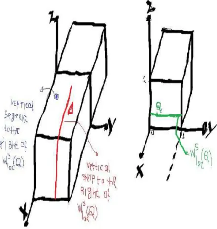
The Affine Blender 13

Figure 4.2: On red color we have vertical strip and on blue a vertical segment

Then we get D_∩F(D_{) =}V_1∪V_{2 and} D_∩F−1₍D_{) =}H_1∪H_{2 (disjoint unions !).} Note that

F−1(u, v, w) =

₄u

5 , f−

1_{(v, w); se (u, v, w)∈V} 1; 4u

5 + 2 5, f−

1_{(v, w); se (u, v, w)∈V} 2.

See figure 2.2.

So let us prove the existence of Blender.

Claim1. F has an unique hyperbolic fix point Qin V_{1 whose index is equal 2,that is, dimW}u_{(Q) = 2.}

In fact, we take Q = (0, q) = (0, y0, z0) where q is the fix point of f in V1. Then F(Q) = F(0, y0, z0) = (0, f(y0, z0)) = (0, y0, z0) =Q and obviously Q∈V1.

LetWs

The Affine Blender 15

Now consider the sets

X± _{:={±1} ×[0,1]×[0,1]}

Y+_{:= [−1,1]× {0} ×[0,1]}

Y−_{:= [−1,1]× {1} ×[0,1]}

Z+_{:= [−1,1]×[0,1]× {1}}

Z−_{:= [−1,1]×[0,1]× {0}}

∂uuD_=Z+_∪Z−_;

∂uD_=X+_∪X−_∪Z+_∪Z−_;

∂s_D=Y+

∪Y−. Claim 2. V_1∩∂s_D=∅;

In fact, this follows from the construction of horseshoe (f, B) where we have I1 ⊂Int([0,1]).

Claim 3. V_1∩F(∂uD_{) =∅;}

Of course, if there is (u, v, w)∈ V_1∩F(∂uD_{)⇒(u, v, w) =F(x, y, z) where (x, y, z)∈∂}uD_{. Then x=±1 and} (4u

5 ,3v,

w

3) = (±1, y, z)⇒u=± 5

4 absurd!

Claim 4. V_2∩∂s_D=∅;

In fact, otherwise we should have _{0,1_{} ∩}I2 6=∅ an absurd!

Claim 5. V_2∩F(∂uu_{D) =∅;}

Of course,By construction of the Smale’s horseshoe (f, B) we have that f(∂uu_{B) =f([0,1]}

×(_{0_{} ∪ {}+1_})) has no intersection with B. Then by construction of F we have the result.

Now note that as F is affine in D_∩F(D_{) =}V_{1 ∪}V_{2 and the tangent space is decomposed in one unstable} plane XLZ where Z is the strong unstable direction and X is the weak unstable direction, and the stable direction which is Y-direction. This implies immediately that F satisfies the hyperbolicity conditionH3 in the definition of blender .Actually the maximal invariant set of F inD _{is hyperbolic set for F.}

Claim 6. There is a neighborhoodU− _{of the face{−1} ×[0,1]×[0,1] of}D_{such that every vertical segment}

L to the right of W_D(s _{Q) has no intersection with U}−_.

Of course,in this case any vertical segment to the right of W_D(s _{Q) is exactly a segment of straight line parallel}

to z-axis and it is far from that face.

Claim 7. For every vertical segment to the right of W_D(s _{Q) one of the two things holds:}

• f(L)∩V_{1 is a vertical segment to the right of WD(}s _Q); • f(L)_∩V_{2 is a vertical segment to the right of WD(}s _Q).

Of course,If L is a vertical segment to the right of W_D(s _{Q) then L = {t} × {y} ×[0,1] with t > 0. Thus the}

x-coordinate of f(L)_∩V_{1 is} 5t

4 and the x-coordinate of f(L)∩V2 is 5t

4 − 1

2. Then we have two possibilities: If t < 4₅ then we get f(L)∩V_{1 to the right of WD(}s _Q).

If 4

5 ≤t≤1 then we get 5t

4 − 1 2 >

1

2 and from thatf(L)∩V2 is to the right of W

s

D(Q).

• f(L)∩V_{1 is disjoint of O}+_; • f(L)∩V_{2) is disjoint ofV.}

In fact, suppose this is not true. Then we can find a sequence Ln of vertical segment to the right ofWD(s Q) such

that as n _{→ ∞} we have limn→∞Dist(F(Ln)∩V1, X+) = 0 = limn→∞Dist(F(Ln)∩V2, WD(s Q)). So denote by

Li

n = F(Ln∩Vi , xin the x-coordinate of Lin where i = 1,2 and xn the x-coordinate of Ln. Since F preserves

vertical directions then we must have limn_→∞x1n = 1 and limn_→∞x2n = 0. On the other hand by using the

definition of F−1 _inV

1∪V2 we must have xn= 4 x1

n 5 =

4x2 n 5 +

2

5. It follows that the sequencexn has two different limits which impossible.

Note that the segments F−1_(L1

n) =Ln∩H1 and F−1(L2n) =Ln∩H2 must have the same x-coordinate. Hence the pair (F,D_{) satisfies the blender conditions.}

Now let us prove directly the main properties of blenders to (F,D_).

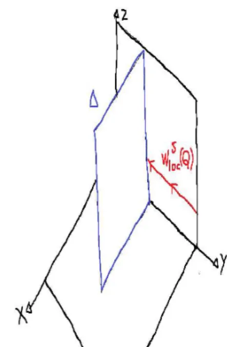
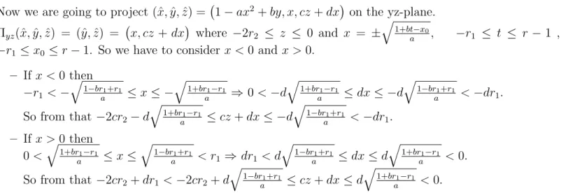
Lemma 4.1.1 If ∆ is a vertical strip to the right of Ws

loc(Q) then either F(∆) intersects Wlocs (Q) or else

F(∆)∩D _{must contain another vertical strip ∆}b _{to the right of W}s

loc(Q) with w(∆) =b 54w(∆).

Proof: Let ∆ = [x1, x2]× {y} ×[0,1] be a vertical strip to the right ofWlocs (Q).

Denote ∆1 =F(∆)∩V1 ⊂D∩F(D) and ∆2 =F(∆)∩V2 ⊂D∩F(D). ThenF−1(∆1) = ∆∩F−1(V1) = ∆∩H1. It follows that we must have F−1_(∆

1) = ∆∩H1 = [x1, x2]× {y} ×[0, z]. So by definition of F the strip ∆1 has

wd(∆1) = 5x₄2−5x₄1. On the other hand we have F−1(∆2) = ∆∩F−1(V2) = ∆∩H2 which implies inF−1(∆2) = ∆_∩H_{2 = [x1, x2]× {y} ×[0, z]. So again by definition of F the strip ∆2 has wd(∆2) = (}5x2

4 − 1 2)−(

5x1 4 −

1 2). Now We have the following cases:

CASE 1 :If x2 ≤ 4₅, then [5₄x1,5₄x2] ⊂ (0,1] and this implies that ∆1 must be a vertical strip to the right of

Ws

loc(Q) and more w(∆1) = 5₄w(∆).

CASE 2: If 4₅ < x2 ≤1 then 5₄x2−1₂ ∈(₂1,3₄].By definition ofF there exists a y′ such that ∆2 =F(∆)∩V2 = [5₄x1− 1₂,5₄x2− 1₂]× {y′} ×[0,1].This gives us more two subcases.

CASE 2.1 :If ₄5x1−1₂ >0 then ∆2 shall be a vertical strip to the right ofWlocs (Q) with widthw(∆2) = 5₄w(∆). CASE 2.2 : If 5₄x1− 1₂ ≤ 0 then ∆2 meets Wlocs (Q) because W

s

loc(Q) = {0} ×[0,1]× {z0} and the proof is

concluded.

Lemma 4.1.2 For any vertical strip ∆ to the right of Ws

loc(Q) there exists an integer n >0 such that Fn(∆)

intersects Ws

loc(Q). In particular every vertical strip ∆to the right of Wlocs (Q)intersects Ws(Q). See figure 4.3.

Proof: Let ∆ be a vertical strip to the right ofWs

loc(Q).If F(∆) intersects Wlocs (Q) it is finished.Otherwise, as

we know there is a vertical strip ˆ∆1 to the right ofWlocs (Q) so that ˆ∆1 ⊂F(∆)∩Bandω( ˆ∆1) =

5

4ω(∆).IfF( ˆ∆1) intersects Ws

loc(Q) it is finished because F( ˆ∆1)⊂F2(∆)∩F(B)⊂F2(∆).Otherwise there is a vertical strip ˆ∆2 to the right of Ws

loc(Q) such that ˆ∆2 ⊂F( ˆ∆1∩Bandω( ˆ∆2) = 54ω( ˆ∆1) = ( 5 4)

2_{ω(∆).IfF( ˆ∆}

2) intersectsWlocs (Q)

it finished since F( ˆ∆2) ⊂ F( ˆ∆1)∩F(B) ⊂ F3(∆)∩F2(B) ⊂ F3(∆). Otherwise we may apply the previous proposition again and since 5₄ >1 it follows that for somen >0 we shall obtain a vertical strip ˆ∆n to the right

of Ws

loc(Q) such that ω( ˆ∆n) = (5₄)nω(∆)>1 and ˆ∆n ⊂F( ˆ∆n−1)⊂Fn(∆).Hence for some n >0 Fn(∆) must intersects Ws

Blender in the Henon-Like Family 17

Figure 4.3: vertical strip eventually intersects stable manifold

4.2

Blender in the Henon-Like Family

On this section our main objective is study the blender structure for the non-normally H´enon-like family defined as follows.

Definition 4.2.1 (Non-Normally Henon-Like Family)Consider the function ϕ :R4_×R3 _→R3 _{given by}

ϕ((a, b, c, d),(x, y, z)) = (1− ax2 _{+by, x, cz +dx). Thus for each point (a, b, c, d) ∈ R}4 _{one have a smooth}

function,which we shall call ϕ too, given by ϕ(x, y, z)) = (1₋ax2 _{+by, x, cz +dx) and this family depends}

smoothly on the parameters (a, b, c, d)

Let us now state the main result of the reference [1] which is the following theorem:

Theorem 4.2.1 There exists a constant 0< δ < 1

4 such that if the parameters a, b, c and d satisfies:

      

0<|b|< δ;

a > 15(1+₄|b|)2; _P._C

1 +|d|< c < 10₉; 0<_|d_|< 1

9.

Then each diffeomorphisim ϕ has a blender Λ = T_n∈Zfn(D), for some cube D ⊂ R3, containing a saddle fix

point p= (xp, yp, zp) with index 2 and satisfying

dim Πyz Ws(p)

∩D _{= 2.}

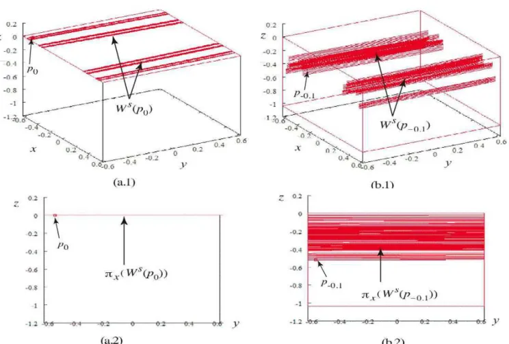
Remark 4.2.1 Numerical simulations in figure 4.4 also support this main theorem. In fact,although uniformly hyperbolicity of ϕ does not break down under (_P._C, geometrical dispersions of stable segment abruptly occurs if

d cross 0, which corresponds to the phase transition from the non-normally hyperbolic horseshoe to the blenders.

Figure 4.4: (a.1) Stable segments forϕa,b,c,d ford= 0 and (a.2) their projective images on theyz-plane , (b.1) Stable

segments for ϕa,b,c,d when d = −0.1 and (b.2) their projective images on the yz-plane ,where (a, b, c) is fixed near

Blender in the Henon-Like Family 19

When in the family above we haveb 6= 0 andc6= 0,then each functionϕ :R3 _→R3 _{is a diffeomorphism.} In fact, it is easy verify that ϕ is a bijective function. Moreover in any point (x, y, z) the jacobian matrix is

Jϕ(x, y, z) =



−21ax 0b 00

d 0 c

 

whose determinant is detJϕ(x, y, z) = ₋bc ₆= 0. So from now on we shall consider only the case b ₆= 0 and

c6= 0 and with that we have a family of diffeomorphism .

Does that family ϕ(x, y, z) = (1₋ax2_{+by, x, cz+dx) have some fix point ?}

Well _

   

1−ax2+by =x x=y

cz+dx=z

⇒     

1−ax2+by−x= 0

x=y

(1−c)z =dx

⇒     

x= (b−1)± √

4a+(b₋1)2 2a

y=x

(1₋c)z =dx

Thus if we have d₆= 0 then z ₆= 0 andc= 1 because₆ x₆= 0 since (x, y, z) is a fix point.So in the case d₆= 0 the point (x, y, z) is a fix point of ϕ if and only if

    

x= (b−1)± √

4a+(b₋1)2 2a

y=x z = dx

1−c

In the case d= 0 the fix point must be only

    

x= (b−1)± √

4a+(b₋1)2 2a

y=x z = 0

For now suppose d₆= 0 and let (x0, y0, z0) be the fixed point of ϕ. Then

Jϕ(x, y, z) =



(1−b)± p

4a+ (1₋b)2 _{b 0}

1 0 0

d 0 c

 

which gives us the characteristic polynomial

P+(λ) = det



(1−b) + p

4a+ (1₋b)2_{−λ b 0}

1 ₋λ 0

d 0 c−λ

 

⇒P+(λ) = −λ3+p4a+ (1−b)2+c+ 1−bλ2+b(1 +c)−c1 +

p

4a+ (1₋b)2_λ−bc. For the other case we obtain

P₋(λ) = det



(1−b)− p

4a+ (1−b)2_{−λ b 0}

1 −λ 0

d 0 c₋λ

 

Lemma 4.2.1 There exists 0 < δ < 1₄ such that if the family ϕ(x, y, z) satisfies P.C then ϕ(x, y, z) = (1−ax2_{+by, x, cz+dx) has a fixed point p= (x}

0, y0, z0) of index 2.

Proof: We already saw that if d6= 0 then the points of coordinates

x=y= (b−1)±

p

4a+ (b₋1)2

2a , z=

d

1₋cx

are fixed points of ϕ.

Consider the fix point of coordinates

x=y= (b−1)−

p

4a+ (b−1)2

2a , z=

d

1₋cx

As we know the characteristic polynomial of the jacobian matrix of ϕ at this fixed point is

P₋(λ) = −λ3+ [(1−b+c)−p4a+ (1−b)2_]λ2_{+ [b(1 +c)−c(1−}p_{4a+ (1−b)}2_)]λ−bc • Claim 1: P₋(λ) has at least one real root in the interval (₋1,1)

In fact, we have that:

P₋(1) = −1 + (1−b+c)−p4a+ (1−b)2_+b+bc−c+cp_{4a+ (1−b)}2_−bc= = (c₋1)p4a+ (1₋b)2

Since c >1 it follows that P₋(1) >0. On the other side we have that:

P₋(₋1) = 1 + 1₋b+c₋p4a+ (1₋b)2_{−b−bc+c−c}p_{4a+ (1−b)}2_−bc= = 2(1₋bc₋b+c)₋(c+ 1)p4a+ (1₋b)2 ₌

= 2(1₋b)(1 +c)₋(c+ 1)p4a+ (1₋b)2 Therefore

P₋(₋1)<0_⇔

2(1₋b)<p4a+ (1₋b)2 _⇔ 4(1₋2b+b2)<4a+ 1₋2b+b2 _⇔

3(1−b)2 4 < a

But by P.C we have a > 15(1+₄|b|)2 > 3(1−₄b)2 which implies P₋(−1)<0.

Hence by Intermediate Value Theorem for Continuous Functions follows that the claim is true.

• Claim 2: P₋(λ) has at least one real root in the interval (1,+_∞).

In fact, since P₋(1)>0 and limλ→+∞P(λ) = −∞this claim is true by Intermediate Value Theorem.

• Claim 3: P₋(λ) has at least one real root in the interval (_−∞,₋1).

Blender in the Henon-Like Family 21

Hence since we have a polynomial of degree 3 then by the claims above the fix point of coordinates

x=y= (b−1)−

p

4a+ (b−1)2

2a , z=

d

1−cx

must be hyperbolic and its index is equal 2. Now let us make some conventions. 1. r1 :=

3(1+|b|)+2√4a+(1+|b|)2

4a ;

2. r2 := |

d_||(b₋1)−√4a+(b₋1)2 | 2a(c₋1)

3. D_{= [−r1, r1]×[−r1, r1]×[zp−r2, zp+r2], where (x0, y0, z0) is the fixed point on of the lemma 4.2.1. As} we can see D _{depends on the parameters (a, b, c, d);}

4. X+ _:=D∩({r

1} ×R2) and X− :=D∩({−r1} ×R2); 5. Y+ _{:=D∩(R× {r}

1} ×R) and Y− :=D∩(R× {−r1} ×R); 6. Z+_:=D∩(R2 _{× {z}

0+r2}) and Z− :=D∩(R2× {z0−r2}).

Lemma 4.2.2 The followings holds(see figure 4.5): (I) |b|+1+

√

4a+(|b|+1)2

2a < r1 <

4 5;

(II) d <0_⇒Z− _⊂R2 _{× {−2r2} and Z}+_⊂R2_{× {0};}

(III) d >0_⇒Z−_⊂(R2_{× {0})∩}D _{and Z}+ _⊂(R2 _{× {2r2})∩}D_.

Proof: (I) The inequality |b|+1+ √

4a+(|b_|+1)2

2a < r1 is immediate as a consequence of the definition of r1.

So let us prove that r1 < 4₅.

0<|b|< δ < 1₄ a > 15(1+₄|b|)2 ⇒

1 +_|b_|< 5₄

1 4a <

1 15(1+|b|)2 <

1 15

So ₁₆1_a2 < 1

225. Thus :

r1 =

3(1 +_|b_|) 4a + 2

r

(1 +_|b_|)2 16a2 +

1 4a <3

1 15

5 4 + 2

r

1 225(

5 4)

2₊ 1 15 =

1 4 + 2

r

53 720 <

4 5 . (II) Suppose we have (x, y, z)_∈Z−_{. Then z =z}

0 −r2 where

z0 =

d(b₋1)−√4a+(b₋1)2

2a(1−c) and r2 =

−db₋1−√4a+(b₋1)2

2a(c₋1) . It follows that:

z = d

2a(1₋c)

(b₋1)₋p4a+ (b₋1)2_{−(b−1)−}p_{4a+ (b−1)}2₌

d

2a(1−c)

2(b₋1)₋p4a+ (b₋1)2_{|] =−2r} 2 ⇒ ⇒(x, y, z)_∈(R2_{× {−2r2})∩}D_.

Blender in the Henon-Like Family 23

Lemma 4.2.3 Suppose that the family ϕ(x, y, z) satisfies the P.C with d 6= 0

1. If d <0 then the set ϕ(D_)∩D _{possesses two connected components} A _and B _on D _{such that:} • A_∩Y+_∪ϕ(X+_∪Z+_)=∅;

• A_∩Y−_∪ϕ(X−_∪Z−_)=∅;

• B_∩(Y+_∪Z+_)∪ϕ(X+_∪Z−_{) =∅;} • B_∩(Y−_∪Z+_)∪ϕ(X−_∪Z−_{) =∅}

2. If d >0 then the set ϕ(D_)∩D _{possesses two connected components} A _and B _on D _{such that:} • A_∩Y+_∪ϕ(X+_∪Z+_)=∅;

• A_∩Y−_∪ϕ(X−_∪Z−_)=∅;

• B_∩(Y+_∪Z−_)∪ϕ(X+_∪Z−_{) =∅;} • B_∩(Y−_∪Z−_)∪ϕ(X−_∪Z−_{) =∅.}

Proof: Ifd <0 we fixed some special points in the edge of D_.

• P1 := (0,−r1,0) P2 := (0,−r1,−2r2);

• P1± := (±r1,−r1,0) P2± := (±r1,−r1,−2r2); • Q1 := (0, r1,0) Q2 := (0, r1,−2r2);

• Q±₁ := (±r1, r1,0) Q±2 := (±r1, r1,−2r2); In the figure 4.6 we can see that points in D_.

Now consider Πxy :R3 →R2 the projection in the xy-plane. Then Πxy ◦ϕ(x, y, z) = (1−ax2+by, x,) that is ,

the projection on the xy-plane gives us the Henon-Family.Let us analyze the points : • Πxy◦ϕ(P1) = (1−br1,0);

• Πxy◦ϕ(P1−) = (1−ar21−br1,−r1) = Πxy ◦ϕ(P2−); • Πxy◦ϕ(P1+) = (1−ar21−br1, r1) = Πxy ◦ϕ(P2+); • Πxy◦ϕ(Q−1) = (1−ar12+br1, r1) = Πxy ◦ϕ(Q−2); • Πxy◦ϕ(Q+₁) = (1−ar₁2+br1, r1) = Πxy ◦ϕ(Q+₂);

• Πxy◦ϕ(Q1) = (1 +br1,0);

Blender in the Henon-Like Family 25

• Claim 1: 1−ar2

1 +|b|r1 <−r1. In fact ,we have that r1 =

3(1+|b_|)2

+2√4a+(1+|b_|)2

4a . Thus 1−ar

2

1+|b|r1 <−r1 ⇔1−ar12+ (1 +|b|)r1 <0⇔ ⇔1₋9(1+|b|)

2

+12(1+|b_|)√4a+(1+|b_|)2 +16a

16a

+3(1+|b|) 2

+2(1+|b_|)√4a+(1+|b_|)2

4a <0⇔

⇔1₋9(1+|b|) 2

+12(1+|b_|)√4a+(1+|b_|)2 16a

−16a

16a +

3(1+|b_|)2

+2(1+|b_|)√4a+(1+|b_|)2

4a <0⇔

⇔ 3(1+|b|) 2

−4(1+|b_|)√4a+(1+|b_|)2

16a <0⇔

↔3(1 +_|b_|)<4p4a+ (1 +_|b_|)2_{. But this last inequality is true by the parameters conditions.} As 1₋ar2

1 ±br1 ≤1−ar21+|b|r1.It follows from the previous claim that 1−ar12±br1 <−r1.

This shows that all of the points Πxy ◦ ϕ(P₁±),Πxy ◦ϕ(P₂±),Πxy ◦ϕ(Q±₁) and Πxy ◦ ϕ(Q±₂) lies in the

semi-plane _{(x, y)_∈R2_{/x <−r1}.}

• Claim 2: Πxy◦ϕ(Y+) is a quadratic curve between the points Πxy◦ϕ(Q−1) = Πxy◦ϕ(Q−2), Πxy◦ϕ(Q+1) = Πxy◦ϕ(Q+₂) and whose critical point is Πxy◦ϕ(Q1) = Πxy ◦ϕ(Q2).

Of course ,as Y+_{={(x, y, z)∈D/y =r}

1} then given (x, y, z)∈Y+ ⇒ ⇒ϕ(x, y, z) = (1₋ax2_+br

1, x, cz+dx)⇒Π◦ϕ(x, y, z) = (1−ax2+br1, x).But (x, y, z)∈D⇒ |x| ≤r1. On this way we have:

– when x=₋r1 ⇒Π◦ϕ(x, y, z) = (1−ar21+br1,−r1);

– when x= 0_⇒Π_◦ϕ(x, y, z) = (1 +br1,0);

– when x=r1 ⇒Π◦ϕ(x, y, z) = (1−ar21+br1, r1); which means that the quadratic curve (1₋ax2_+br

1, x) pass by the points Πxy◦ϕ(Q−₁) = Πxy◦ϕ(Q₂−) = (1−ar₁2+br1,−r1),

Πxy◦ϕ(Q+1) = Πxy◦ϕ(Q+2) = (1−ar12+br1, r1) and Πxy◦ϕ(Q1) = Πxy ◦ϕ(Q2).

See the figure 2.7

• Claim 3:Πxy◦ϕ(Y−) is a quadratic curve between the points Πxy◦ϕ(P1−) = Πxy ◦ϕ(P2−), Πxy◦ϕ(P1+) = Πxy◦ϕ(P2+) and Πxy◦ϕ(P1) = Πxy◦ϕ(P2.)

Of course, as Y+_{={(x, y, z)∈D/y =−r}

1} then given (x, y, z)∈Y− ⇒ ⇒ϕ(x, y, z) = (1₋ax2_+br

1, x, cz+dx)⇒Π◦ϕ(x, y, z) = (1−ax2−br1, x). This sows that Πxy◦ϕ(Y−)

is a quadratic curve.In another side (x, y, z)_∈Y− _{⇒ |x| ≤r}

1. Thus

– when x=₋r1 ⇒Π◦ϕ(x, y, z) = (1−ar21−br1,−r1);

– when x= 0⇒Π◦ϕ(x, y, z) = (1−br1,0) and

– when x=r1 ⇒Π◦ϕ(x, y, z) = (1−ar21−br1, r1). But

Πxy◦ϕ(P1−) = Πxy ◦ϕ(P2−) = (1−ar21−br1,−r1), Πxy◦ϕ(P₁+) = Πxy ◦ϕ(P₂+) = (1−ar2₁−br1, r1), Πxy◦ϕ(P1) = Πxy ◦ϕ(P2) = (1−br1,0).

See the figure 2.7

• Claim 4: Πxy◦ϕ(Ω) is a quadratic curve between the curves Πxy◦ϕ(Y+) and Πxy ◦ϕ(Y−).

In fact, if (x, y, z) ∈Ω then ϕ(x, y, z) = (1−ax2_+br

1, x, cz+dx) ⇒ Π◦ϕ(x, y, z) = (1−ax2+brδ, x). This sows that Πxy ◦ϕ(Ω) is a quadratic curve.

Now as

Πxy ◦ϕ(Y+) = (1−ax2+br1, x),|x| ≤r1 Πxy ◦ϕ(Y−) = (1−ax2−br1, x),|x| ≤r1. and we have ₋r1 < δ < r1 then

– If b >0_{⇒ −}br1 < bδ < br1 ⇔1−ax2−br1 <1−ax2+bδ <1−ax2+br1.

– If b <0 and−r1 <0< δ < r1 then br1 < bδ <0<−br1 ⇔ ⇔1₋ax2_+br

1 <1−ax2+bδ <1−ax2−br1.

The following figure shows Πxy ◦ϕ(D) in the caseb <0 and d <0.

Since the connectedness is invariant by continuous functions we obtain that D_∩ϕ(D_{) must possesses two} connected components in D_.

Now we are going to determine the projection of D _{and ϕ(}D_{) in the xz-plane,that is ,the sets Πxz(}D_{) and} Πxz◦ϕ(D). As we haved <0 it is immediate verify that Πxz(D) is the rectangle [−r1, r1]×[zp−r2, zp+r2] = [−r1, r1]×[−2r2,0]. Also is immediate verify that

– Πxz◦ϕ(P1) = (1−br1,0) , Πxz◦ϕ(P2) = (1−br1,−2cr2);

– Πxz◦ϕ(Q1) = (1 +br1,0) , Πxz◦ϕ(Q2) = (1 +br1,−2cr2);

– Πxz◦ϕ(P1−) = (1−ar12−br1,−dr1);

– Πxz◦ϕ(P2−) = (1−ar12−br1,−2cr1−dr1);

– Πxz◦ϕ(P1+) = (1−ar12−br1, dr1);

– Πxz◦ϕ(P2+) = (1−ar12−br1,−2cr1+dr1);

– Πxz◦ϕ(Q−1) = (1−ar12+br1,−dr1);

– Πxz◦ϕ(Q−2) = (1−ar12+br1,−2cr1−dr1);

– Πxz◦ϕ(Q+₁) = (1−ar₁2+br1, dr1);

– Πxz◦ϕ(Q+2) = (1−ar12+br1,−2cr1+dr1);

• Claim 5: The segment of line between Πxz◦ϕ(P1) and Πxz◦ϕ(P1−) has no intersection with the segment Πxz(Z+).

Of course,as Z+ _{= {(x, y, z) ∈ D/z = z}

p +r2} then Πxz(Z+) = {(x, z) ∈ R2/|x| ≤ r1, z = zp +r2} = {(x,0)_∈R2_{/|x| ≤r1} since by Claim 1 which precedes the proposition 1 we have Z}+ _⊂R2_{× {0}.}

The segment of line between Πxz ◦ϕ(P1) and Πxz ◦ϕ(P1−) is given by : {tΠxz◦ϕ(P1) + (1−t)Πxz◦ϕ(P₁−)}=

=_{((1₋br1)t,0) + ((1−t)(1−ar12−br1),−(1−t)dr1)/t∈[0.1]}= {([1₋br1]t+ [1−t][1−ar21−br1],[t−1]dr1)/t∈[0,1]}.

Blender in the Henon-Like Family 27

• Claim 6 : dr1 >−2r2.

In fact, as dr1 >−2r2 ⇔ −dr1 <2r2 ⇔ |d|r1 <2r2 = 2|d_c−||x₁p| ⇔r1 < 2_c|₋xp₁| ⇔ ⇔3(1 +|b|) + 2p4a+ (1 +|b|)2 _< 2[(1−b)+

√

4a+(1−b)2_] 2a(c−1) ⇔ ⇔3(1 +|b|) + 2p4a+ (1 +|b|)2 _< 4[(1−b)+

√

4a+(1−b)2]

c−1 .

Thus it is enough show the following inequality ⇔3(1 +|b|) + 2p4a+ (1 +|b|)2 _< 4[(1−b)+ √

4a+(1−b)2]

c−1 ⇔

⇔(c₋1)[3(1 +_|b_|) + 2p4a+ (1 +_|b_|)2_{]<4[(1− |b|) +}p_{4a+ (1− |b|)}2_].

By parameters conditions c₋1> 1₉ and thus the last inequality is true since the inequality 3(1+|b_|)+2√4a+(1+|b_|)2

9 <4[(1− |b|) +

p

4a+ (1_{− |}b_|)2_]⇔

3(1 +_|b_|) + 2p4a+ (1 +_|b_|)2 _{<36(1− |b|) + 36}p_{4a+ (1− |b|)}2 _{(∗∗) is true.} Finally (_∗∗) will be true since the followings inequalities hold.

(α) 36p4a+ (1_{− |}b_|)2 _>2p_{4a+ (1 +|b|)}2 (β) 36(1− |b|)>3(1 +|b|).

But (α) is true iff 182_{[(1− |b|)}2_{+ 4a]>(1 +|b|)}2_{+ 4a⇔4a(18}2_{−1)>(1 +|b|)}2₋₁₈2_{(1− |b|)}2 _⇔ ⇔4a > (1+|b|)2₁₈−182 2(1−|b|)2

−1 ⇔4a >

1+2|b|+|b|2

−324(1−2|b|+|b|2 )

323 ⇔4a >

−323|b|2

+650|b|−323

323 ⇔

⇔4a >_−|b_|2₊ 650|b_|

323 −1 which is true by parameter condition.

On the other side ,the inequality on (β) is true iff 33 ≥ 39|b| and this last is true again by parameters conditions.

• Claim 7: The segment of line between Πxz◦ϕ(P1) and Πxz◦ϕ(P1+) not intersects the segment Πxz(Z+).But

it intersects the segments Πxz(X+) and Πxz(X−) passing trough the interior of Πxz(D).

In fact ,as we have d <0 then by claim 1 before the proposition 1, we obtain Πxz(D) ={(x, z)∈R2/|x| ≤r1 and −2r2 ≤z ≤0}

Since Πxz◦ϕ(P1) = (1−br1,0) and Πxz◦ϕ(P₁+) = (1−ar₁2−br1, dr1) then from 1±br1 ≥1−|b|r1 > 4₅ > r1we see that Πxz◦ϕ(P1) is not onP ixz(D). On the other hand from claim 1 above 1−ar12±br1 ≤1−ar21+|b|r1 <

r1 implies that Πxz◦ϕ(P1+) is not on Πxz(D). So from that and from claim 6 above the result follows.See

figure 4.7

• Claim 8 : −2cr2−dr1 <−2r2.

In fact, this is immediate from the claim 6 above .

• Claim 9 : The segment of line between Πxz◦ϕ(P2) and Πxz◦ϕ(P2−) has no intersection with the segment Πxz(Z−).

Of course, we have Πxz(Z−) = {(x,−2r2)/|x| ≤r1}, Πxz◦ϕ(P2) = (1−br1,−2cr2) and

Πxz◦ϕ(P2−) = (1−ar12−br−1,−2cr2−dr1). Thus the segment of line between Πxz◦ϕ(P2) and Πxz◦ϕ(P2−) is the set

ˆ

S := {(t[1−br1] + [1−t][1−ar21 −br1],−2tcr2+ [1−t][−2cr2 −dr1])/t ∈ [0,1]} so one point of ˆS also belongs to Πxz(Z−) iff there exists t0,0≤t0 ≤1 such that

−2t0cr2 + [1 −t0][−2cr2 −dr1] = −2r2 ⇔ t0 = 2cr2+_drdr₁1−2r2. But d < 0 and r1 > 0 which means that

t0 ∈[0,1] implies in 2cr2+dr1 ≤2r2 what is a contradiction by claim 8 above.

• Claim 10 : The segment of line between Πxz◦ϕ(P2) and Πxz◦ϕ(P₂+) has no intersection with the segment