Taxonomic reference libraries for environmental barcoding: a best practice example from diatom research.

(1)

Taxonomic Reference Libraries for Environmental

Barcoding: A Best Practice Example from Diatom

Research

Jonas Zimmermann1,2*"_{, Nelida Abarca}1"

, Neela Enk1", Oliver Skibbe1,3, Wolf-Henning Kusber1, Regine Jahn1

1Botanic Garden and Botanical Museum Berlin-Dahlem, Freie Universita¨t Berlin, Berlin, Germany,2Justus-Liebig-Universita¨t Giessen, AG Spezielle Botanik, Giessen, Hessen, Germany,3Larger than life - micro and nature photography, http://www.larger-than-life.de, Berlin Germany

Abstract

DNA barcoding uses a short fragment of a DNA sequence to identify a taxon. After obtaining the target sequence it is compared to reference sequences stored in a database to assign an organism name to it. The quality of data in the reference database is the key to the success of the analysis. In the here presented study, multiple types of data have been combined and critically examined in order to create best practice guidelines for taxonomic reference libraries for environmental barcoding. 70 unialgal diatom strains from Berlin waters have been established and cultured to obtain morphological and molecular data. The strains were sequenced for 18S V4 rDNA (the pre-Barcode for protists) as well as rbcL data, and identified by microscopy. LM and for some strains also SEM pictures were taken and physical vouchers deposited at the BGBM. 37 freshwater taxa from 15 naviculoid diatom genera were identified. Four taxa from the genera Amphora, Mayamaea,PlanothidiumandStauroneisare described here as new. Names, molecular, morphological and habitat data as well as additional images of living cells are also available electronically in the AlgaTerra Information System. All reference sequences (or reference barcodes) presented here are linked to voucher specimens in order to provide a complete chain of evidence back to the formal taxonomic literature.

Citation:Zimmermann J, Abarca N, Enk N, Skibbe O, Kusber W-H, et al. (2014) Taxonomic Reference Libraries for Environmental Barcoding: A Best Practice Example from Diatom Research. PLoS ONE 9(9): e108793. doi:10.1371/journal.pone.0108793

Editor:Bernd Schierwater, University of Veterinary Medicine Hanover, Germany

ReceivedMay 13, 2014;AcceptedAugust 14, 2014;PublishedSeptember 29, 2014

Copyright:ß2014 Zimmermann et al. This is an open-access article distributed under the terms of the Creative Commons Attribution License, which permits unrestricted use, distribution, and reproduction in any medium, provided the original author and source are credited.

Data Availability:The authors confirm that all data underlying the findings are fully available without restriction. All relevant data are within the paper. The web link to AlgaTerra for all taxa, the DNA Bank number and the EMBL accession numberss are available in Table 2.

Funding:Deutsche Forschungsgemeinschaft (http://www.dfg.de/) grant INST 130/839-1 FUGG. Institution was funded. Deutsche Forschungsgemeinschaft (http://www.dfg.de/) grant GE 12 42/11-1 RJ; JZ is employed on this grant. German Federal Ministry of Education and Research (http://www.bmbf.de/) funding for microscopy data within the GBIF-D project 01 LI 1001 A. The funders had no role in study design, data collection and analysis, decision to publish, or preparation of the manuscript.

Competing Interests:The authors have declared that no competing interests exist.

* Email: j.zimmermann@bgbm.org

"These authors are shared first authors on this work.

Introduction

Diatoms are unicellular and usually photoautotroph micro algae which are responsible for about 25% of global CO2fixation [1–3] and contribute approximately 20% of the global net primary production [4].

Diatoms are important bioindicators for monitoring water quality because they are sensitive to changes in pollution, nutrient availability, acidity and salinity, e.g. [5,6]. They are the most ubiquitous group within the microscopic algae as they occur in all types of water bodies and play an important part in benthic and planktonic biocoenoses [7]. They are routinely used as bioindica-tors within the EU Water Framework Directive (WFD) as well as in water quality monitoring worldwide [8–13].

Each diatom cell is encased in two siliceous shells (frustules) that are connected by girdle bands [1–3]. Current identification of diatoms is based on a morphological and mostly descriptive species concept (Zimmermann et al. subm.) and relies exclusively on micro-characters of the frustule such as size, symmetry, shape, and sculpture which can be seen by light microscopy [14]; more

detailed analyses of the siliceous structures lead to more and more refined differentiation of species, which is possible through the development of higher resolution techniques, e.g. electron microscopy.

Identification via microscopy is challenging and time consum-ing, especially for routine use [15], and relies on individual taxonomic expertise. Therefore different taxonomists could arrive at different conclusions, depending i.a. on the taxonomic concept, species with limited diagnostic morphological features, cryptic species, available reference floras and quality of microscopes used by each individual researcher [15] as well as unavailability of adequate descriptions.

The application of molecular markers for taxon identification – DNA barcoding – is an emerging method which has the potential to be faster, universally applicable and generate reliable identifi-cation. Furthermore, as it uses DNA sequences for identification, it is independent of pre-existing morphological species concepts and can be linked to any taxonomic concept [16]. However, correct identification relies fundamentally on the quality of the reference

(2)

library the DNA barcodes are checked against. DNA barcoding is based on the assumption that sequences of a certain marker locus exhibit enough variation between species to be discriminative for unambiguous species discovery [17,18]. DNA barcoding is also a useful tool to access concealed diversity e.g. [19–25]. DNA barcoding in combination with next generation sequencing techniques also allows for the description of community compo-sitions through the large numbers of sequences generated by this approach e.g. [26,27]. A schematic overview on environmental DNA barcoding of diatoms and the establishment of a reference library is given in Fig. 1.

The requirement for reliable taxon identification by DNA barcode(s) is an unambiguous link between the genotype and the phenotype (or morphotype) to which the name of the species is attached. This means that a reference library consisting of taxon names belonging to specimens that have been identified by experts as well as providing descriptions together with barcode sequences, which were derived from well documented strains (e.g. voucher deposition, sampling localities and collectors, basic environmental data, high-resolution LM pictures, morphometrics, taxonomy and nomenclature, maps, literature and references to databases where this data is deposited) for every single species is necessary. For unicellular diatoms, clone cultures (strains) need to be established which offer enough material for sequencing as well as for identification by light and electron microscopy. Once established and linked to a taxonomic reference library, the DNA barcoding method could offer a time and cost efficient alternative/extension to microscopic identification for routine applications by limiting morphological taxonomy to critical groups which feature a distinct genetic aberration to known and identified organisms in the library.

Recently, the CBOL Protist Working Group [28] has desig-nated the 18S V4 rDNA marker region as first or pre-barcode for Protist organisms. In this paper, we follow the 18S V4 protocols designed for diatoms by Zimmermann et al. [19], and present 70 strains for which this pre-barcode (18S V4) as well as a second widely used barcode, rbcL [20,21,29], has been generated. The reference library includes these two DNA barcodes, the respective taxon name, images, morphometric and geographic data as well as vouchers for further reference. Further data and additional images also of living cells are available electronically through the AlgaTerra Information System [30]. We demonstrate the benefits of a well documented reference library for DNA barcoding for identification, taxonomy, phylogeny, and further scientific analyses on an exemplary group. This paper focuses on naviculoid diatom strains from Berlin waters since its diatom flora has been well studied for almost two centuries by light microscopy [31] and a recent diatom flora is available for water quality assessments [32].

Materials and Methods

Sampling

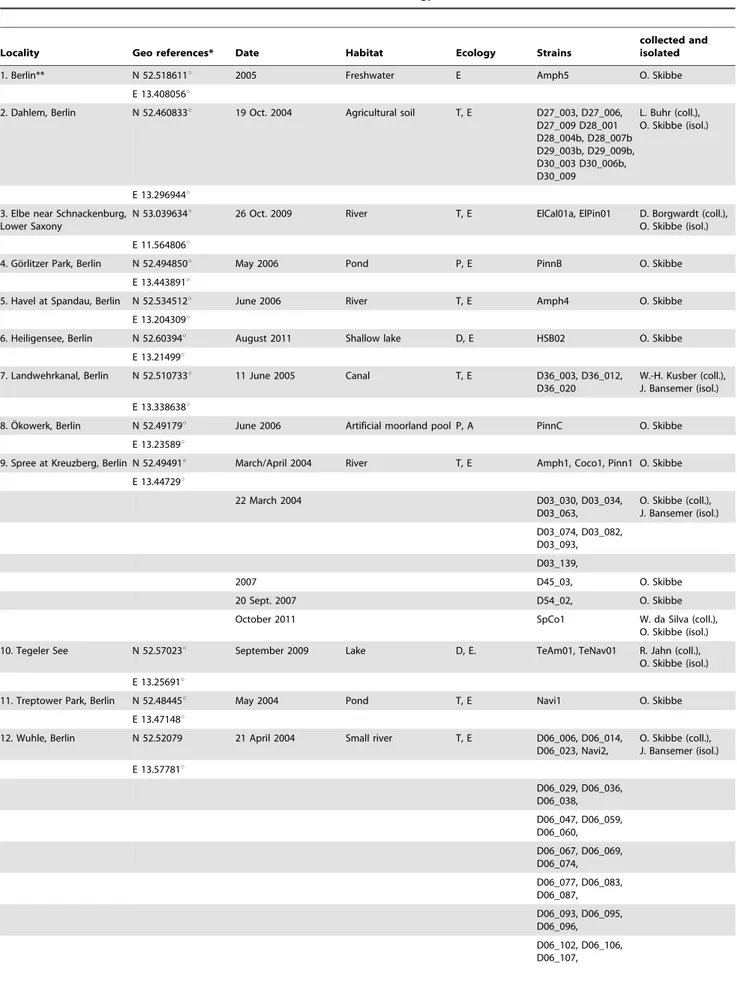
Benthic samples from which the 70 strains were established were collected at 11 sites in the catchment area of Berlin (Fig. 2); one additional sample was from the River Elbe, downstream of the Berlin Rivers Spree and Havel. Conductivity of Berlin water ranges mostly between 400 to 900mS cm21, pH is frequently 6,5 to 9 (80% respectively 88% of about 300 measurements of Berlin water samples, Kusber unpubl. data). For samples, sites, dates, collectors of the samples and isolators of the strains see Table 1. No specific permissions were required for the sampled locations/ activities. The field studies did not involve endangered or protected species.

Cultivation

The diatom cells were isolated from environmental water samples observed under a stereo light microscope using capillary glass pipettes. The respective cell was then transferred to a 5 cm diameter plastic petri dish containing autoclaved habitat water and/or culture medium (WC [33], Chu [34], AlgaGrow, Plagron, Weert, Netherlands) of adequate salinity and pH. In order to remove unwanted particles, this treatment was repeated several times until microscopic inspection confirming that a culture derived from one cell, but not axenic had been established. The cultures were grown at a temperature between 18–22uC and a 12 h day/night cycle.

Preparation of frustules

By the time of harvesting the cultures, one fraction was used for obtaining DNA (see below) and the other part was cleaned with H202at 80uC and rinsed several times with H20. A few drops of the resulting suspension of diatom frustules were dried on a cover slip and embedded as slides in Naphrax for study in LM or on stubs if for SEM. Vouchers of each strain were deposited in the Herbarium Berolinense (B) (see Table 2).

Light and electron microscopy

The LM pictures were acquired with a Zeiss Axio Imager.M2 with an implemented AxioCam HRc (Zeiss, Oberkochen, Germany). SEM pictures were produced with Philips SEM 515 operating at 30 KV (Philips, Eindhoven, The Netherlands), and Hitachi 8010 Field Emission Electron Microscope (Hitachi, Tokyo, Japan).

Identification

The taxa were identified with Hofmann et al. [32], Krammer & Bertalot (1997) [35], Ettl & Ga¨rtner (2013) [36], Lange-Bertalot (2001), Levkov et al. (2009) [37], Levkov et al. (2014) [38] as well as particular papers (vide infra) for selected species. For strain numbers, taxon names, voucher codes in the Herbarium Berolinense (B), EMBL Accession Numbers, images, and mor-phometric data for all strains see Table 2.

DNA isolation

The harvested cultures were transferred to 1.5 ml tubes. DNA was isolated using Dynal DynaBeads (Invitrogen Corporation; Carlsbad, CA, USA), NucleoSpin Plant II Mini Kit (Machery and Nagel, Du¨ren, Germany) or Qiagen Dneasy Plant Mini Kit (Qiagen Inc.; Valencia, CA) following the respective product instructions. DNA concentrations were checked using gel electro-phoresis (1.5% agarose gel) and Nanodrop (PeqLab Biotechnology LLC; Erlangen, Germany). DNA samples were stored at220uC until further use. DNA material was deposited in the Berlin collection of the DNA bank network [39].

PCR amplification

The V4 region of the 18S locus was amplified in all strains with the primer pair M13F-D512 for 18S/M13F-D978rev 18S [19]. TherbcL locus was amplified in two overlapping parts using two different primer pairs; Diat-rbcL-F and Diat-rbcL-iR as well as Diat-rbcL-iF and Diat-rbcL-R [40] for all strains. The polymerase chain reaction (PCR) for the V4 region was conducted after Zimmermann et al. (2011) [19] and for rbcL carried out after Abarca et al. (2014) [40]. PCR products were visualised in a 1.5% agarose gel and cleaned with MSB Spin PCRapace (Invitek LLC; Berlin, Germany) following standard procedure. DNA content was measured using Nanodrop (PeqLab Biotechnology). The samples

Taxonomic Reference Libraries for Environmental Barcoding of Diatoms

(3)

(4)

were normalised to a total DNA content .100 ng/ml using Nanodrop (PeqLab Biotechnology) for further sequencing.

Sequencing

The Sanger sequencing was conducted by Starseq (GENterprise LLC; Mainz, Germany). As sequencing primers the M13 tails [19,41] were used for the V4 region, following [42]. The sequences were edited in PhyDE [43] aligned using MUSCLE [44], and alignments were manually improved in PhyDE [43].

Molecular analysis

The aligned sequences were compared to each other calculating uncorrected p distances in PAUP [45]. Then they were blasted against existing INSDC entries for the respective taxa (accessed July 2013). All INSDC accessions with references are given in Appendix S1. Base pair differences were counted in overlapping

parts of the sequences in Mega 5 [46]. Results are summarised in Table 3.

Tree building

To identify molecular relations between the here presented strains, trees were calculated with Mega 5 using the Neighbour Joining algorithm with gamma distributed rates among sites followed by a statistical test of the tree topologies with 10 000 bootstrap replications. Trees for the individual alignments of 18S V4 andrbcL sets as well as a concatenated dataset were calculated. Furthermore, we created 18S V4 as well as rbcL datasets including INSDC sequences for the generaAmphora,Mayamaea, Planothidium and Stauroneisto exemplarily test the taxonomic consistency of available sequences as well as the placement of our new taxa. Each of these eight datasets was analysed under the aforementioned conditions.

Figure 1. Schematic overview of sample processing and voucher as well as data production and deposition for environmental barcoding.

doi:10.1371/journal.pone.0108793.g001

Figure 2. Map of the sampling localities in the Berlin region. For details to the numbered sampling sites see Table 1. doi:10.1371/journal.pone.0108793.g002

(5)

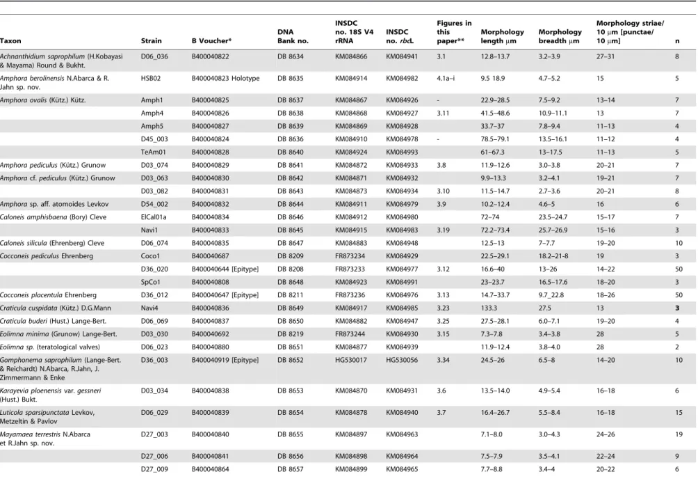
Table 1.List of Localities: Strain Numbers, Geo-Reference, Habitat, Ecology.

Locality Geo references* Date Habitat Ecology Strains

collected and isolated

1. Berlin** N 52.518611u 2005 Freshwater E Amph5 O. Skibbe

E 13.408056u

2. Dahlem, Berlin N 52.460833u 19 Oct. 2004 Agricultural soil T, E D27_003, D27_006, D27_009 D28_001 D28_004b, D28_007b D29_003b, D29_009b, D30_003 D30_006b, D30_009

L. Buhr (coll.), O. Skibbe (isol.)

E 13.296944u

3. Elbe near Schnackenburg, Lower Saxony

N 53.039634u 26 Oct. 2009 River T, E ElCal01a, ElPin01 D. Borgwardt (coll.), O. Skibbe (isol.)

E 11.564806u

4. Go¨rlitzer Park, Berlin N 52.494850u May 2006 Pond P, E PinnB O. Skibbe

E 13.443891u

5. Havel at Spandau, Berlin N 52.534512u June 2006 River T, E Amph4 O. Skibbe

E 13.204309u

6. Heiligensee, Berlin N 52.60394u August 2011 Shallow lake D, E HSB02 O. Skibbe

E 13.21499u

7. Landwehrkanal, Berlin N 52.510733u 11 June 2005 Canal T, E D36_003, D36_012, D36_020

W.-H. Kusber (coll.), J. Bansemer (isol.)

E 13.338638u

8. O¨kowerk, Berlin N 52.49179u June 2006 Artificial moorland pool P, A PinnC O. Skibbe

E 13.23589u

9. Spree at Kreuzberg, Berlin N 52.49491u March/April 2004 River T, E Amph1, Coco1, Pinn1 O. Skibbe

E 13.44729u

22 March 2004 D03_030, D03_034,

D03_063,

O. Skibbe (coll.), J. Bansemer (isol.)

D03_074, D03_082, D03_093,

D03_139,

2007 D45_03, O. Skibbe

20 Sept. 2007 D54_02, O. Skibbe

October 2011 SpCo1 W. da Silva (coll.),

O. Skibbe (isol.)

10. Tegeler See N 52.57023u September 2009 Lake D, E. TeAm01, TeNav01 R. Jahn (coll.), O. Skibbe (isol.)

E 13.25691u

11. Treptower Park, Berlin N 52.48445u May 2004 Pond T, E Navi1 O. Skibbe

E 13.47148u

12. Wuhle, Berlin N 52.52079 21 April 2004 Small river T, E D06_006, D06_014, D06_023, Navi2,

O. Skibbe (coll.), J. Bansemer (isol.)

E 13.57781u

D06_029, D06_036, D06_038,

D06_047, D06_059, D06_060,

D06_067, D06_069, D06_074,

D06_077, D06_083, D06_087,

D06_093, D06_095, D06_096,

D06_102, D06_106, D06_107,

(6)

Nomenclature

The electronic version of this article in Portable Document Format (PDF) in a work with an ISSN or ISBN will represent a published work according to the International Code of Nomen-clature for algae, fungi, and plants, and hence the new names contained in the electronic publication of a PLOS ONE article are effectively published under that Code from the electronic edition alone, so there is no longer any need to provide printed copies. The online version of this work is archived and available from the following digital repositories: PubMed Central, LOCKSS. http:// edocs.fu-berlin.de/docs/content/below/index.xml.

Results

Morphological analyses

The morphological identification of the 70 strains resulted in 37 taxa (see Table 2 and Figs. 3 and 4). 21 taxa were identified by only one strain but 10 taxa were represented by two strains, three taxa by three strains, one taxon by four strains, one taxon by five strains and one taxon by 11 strains.

DNA sequence analyses

PCR and sequencing success for 18S V4 andrbcL was 100% for all strains, resulting in 140 reference sequences for 70 strains. We established 129 novel sequences (INSDC accession numbers KM084866-KM084994) and an additional 11 sequences that had been previously published in Abarca et al. [40] and Zimmermann et al. [19].

There was little molecular variation within the here generated sequence data – only up to 0.5% in 18S V4 (representing 2 bp) and 0.3% inrbcL (corresponding to 3 bp) – between the different strains representing one taxon (Appendix S2). The highest in-taxon variation was found in e.g.Mayamaea terrestris0.53% (18S V4), respectively Navicula cryptocephala e.g. 0.33% (rbcL). The uncorrected p distances for all genera and sequences are given in Appendix S2.

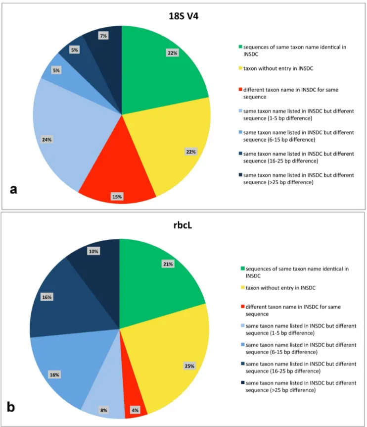
The results from sequence comparison with sequences pub-lished in the databases of the International Nucleotide Sequence Database Collaboration (INSDC, includes GenBank, EMBL and DDBJ) are shown in Table 3 and summarised in Fig. 5a, 5b. In the case of 18S V4, 22% of our taxa had entries with identical sequences in the INSDC whereas forrbcL this number was 21% (Fig. 5b). This was the case e.g. forCaloneis siliculaandNavicula cryptotenella (Table 3). 22% (18S V4, Fig. 5a) respectively 25% (rbcL, Fig. 5b) of our taxa had no entry in the INSDC databases, e.g. Amphora ovalis and Luticola sparsipunctata (Table 3). For 15% of our taxa an identical 18S V4 sequence (Fig. 5a) with a different taxon name was found in the INSDC databases (e.g.

Gomphonema parvulum); the number was considerably lower in rbcL with only 4% (Fig. 5b). The remaining taxa of which many showed sequence dissimilarities of over 15 bp were 41% for 18S V4 (Fig. 5a) and 50% forrbcL (Fig. 5b). The highest difference was found for Pinnularia viridiformis with 97 bp in 18S V4 (Table 3).

The tree derived from the concatenated data set and calculated by the Neighbour Joining (NJ) algorithm, including only the here presented strains, is shown in Fig. 6; the trees of the individual analysis of both markers are given in the Appendix S2. The molecular clades are congruent between 18S V4 andrbcL, the tree topology is partly differing between both markers (Appendix S3, S4); however, the conflicting nodes have bootstrap values below 0.85 and are therefore neglected.

In the tree derived from the combined dataset, the sampled genera are monophyletic and well supported (.0.98 bootstrap support BS, Fig. 6), except forCaloneis,CraticulaandSellaphora. Craticula buderi falls into a clade with the generaStauroneis and Karayevia(0.48 BS; Fig. 6).Sellaphora falls into one group withEolimna(0.98 BS; Fig. 6). The genusCaloneisis found in two distinct clades:Caloneis siliculais clustering withPinnularia(0.61 BS; Fig. 6),Caloneis amphisbaenaforms an independent clade on its own (1.00 BS; Fig. 6). The deeper bifurcations representing the relationship between the genera are generally not well supported by bootstrap values. All 37 subgeneric taxa included in this study are monophyletic (Fig. 6).

The trees for the genus Amphora including all available data from INSDC databases (this includes also accessions from the genusHalamphora) are shown in Fig. 7a (18S V4) and Fig. 7b (rbcL). The Amphora ovalis strains (Amph1, Amph4, Amph5, D45_003 and TeAm01) form a monophyletic clade, that is well supported in both 18S (0.99 BS) andrbcL (0.97 BS). The strain HSB02, identified asAmphora berolinensisappears to be rather isolated within theAmphoratree, except for an affiliation with the unidentified strain C10 (INSDC accession number FJ002132) in therbcL tree (0.89 BS; Fig. 7b). All strains identified asAmphora pediculuscluster in one clade in 18S V4 (0.90 BS; Fig. 7a) and rbcL (Fig. 7b). This includes also the strain D54_002 named Amphorasp. aff.atomoides. The tree derived fromrbcL sequences also includes the strain AT-21.206 (INSDC accession number AN502022) identified asAmphora cf.fogediana (Fig. 7b), which forms a branch with strain s0992 named Amphora copulata (INSDC accession number AB754831) in 18S V4 adjacent to the Amphora pediculusclade (Fig. 7a). In respect to the other strains available from the INSDC databases there is no topology consistent with the taxonomic identifications found in the trees (Fig. 7a, 7b). Several taxa, including the species Amphora coffeaeformis, Amphora normannii and Amphora montana were

Table 1.Cont.

Locality Geo references* Date Habitat Ecology Strains

collected and isolated

D06_110, D06_113, D06_122,

D06_138, D06_139,

April 2004 Navi4, Stau1 O. Skibbe

June 2004 Navi5, Pinn2 O. Skibbe

(Ecology: D = dimictic, P = polymictic, T = turbid, E = eutrophic, alkaline, A = acidic, all running waters are part of Elbe catchment area). *Uncertainty =650 m,

** Uncertainty =622500 m. doi:10.1371/journal.pone.0108793.t001

(7)

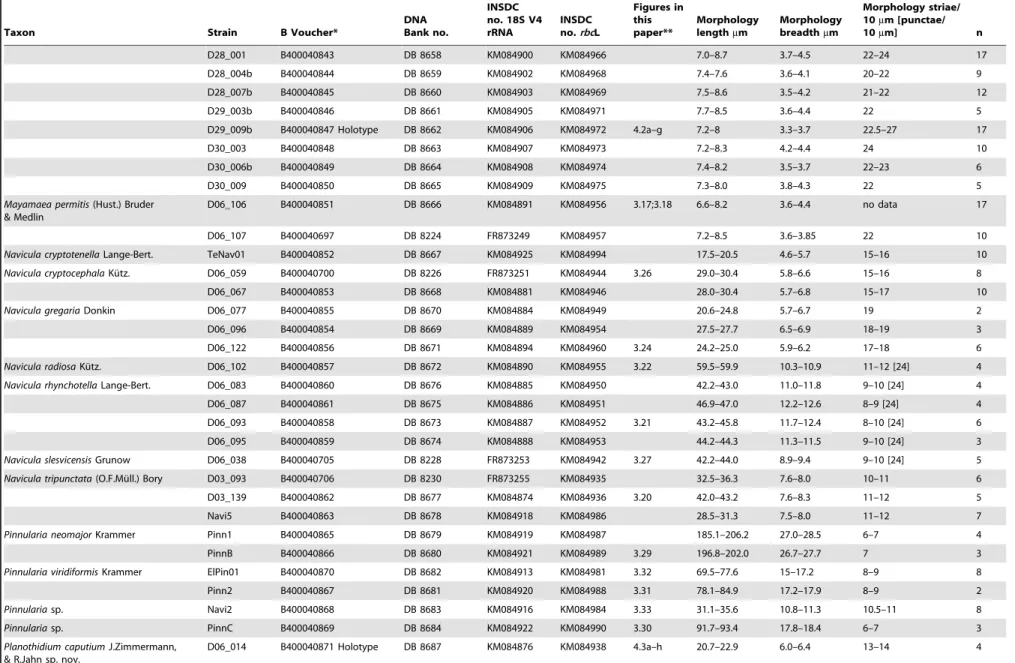
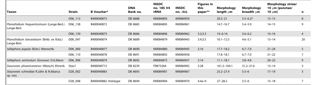
Table 2.List of materials from Berlin localities: names of 37 Taxa and 70 strains, voucher codes in the Herbarium Berolinense (B), DNA Bank voucher numbers in the Berlin-Dahlem Plant DNA Bank, INSDC accession numbers, picture numbers in this publication and morphometrics of each strain (n = number of evaluated valves).

Taxon Strain B Voucher*

DNA Bank no.

INSDC no. 18S V4 rRNA

INSDC no.rbcL

Figures in this paper**

Morphology lengthmm

Morphology breadthmm

Morphology striae/ 10mm [punctae/

10mm] n

Achnanthidium saprophilum(H.Kobayasi

& Mayama) Round & Bukht.

D06_036 B400040822 DB 8634 KM084866 KM084941 3.1 12.8–13.7 3.2–3.9 27–31 8

Amphora berolinensisN.Abarca & R.

Jahn sp. nov.

HSB02 B400040823 Holotype DB 8635 KM084914 KM084982 4.1a–i 9.5 18.9 4.7–5.2 15 5

Amphora ovalis(Ku¨tz.) Ku¨tz. Amph1 B400040825 DB 8637 KM084867 KM084926 - 22.9–28.5 7.5–9.2 13–14 7

Amph4 B400040826 DB 8638 KM084868 KM084927 3.11 41.5–48.6 10.9–11.1 13 7

Amph5 B400040827 DB 8639 KM084869 KM084928 33.7–37 7.8–9.4 11–13 4

D45_003 B400040824 DB 8636 KM084910 KM084978 - 78.5–79.1 13.5–16.1 11–12 4

TeAm01 B400040828 DB 8640 KM084924 KM084993 61–67.3 13–17.5 11–13 5

Amphora pediculus(Ku¨tz.) Grunow D03_074 B400040829 DB 8641 KM084872 KM084933 3.8 11.9–12.6 3.0–3.8 20–21 7

Amphoracf.pediculus(Ku¨tz.) Grunow D03_063 B400040830 DB 8642 KM084871 KM084932 9.9–13.3 3.2–4.1 19–21 7

D03_082 B400040831 DB 8643 KM084873 KM084934 3.10 11.5–14.7 2.7–3.6 20–21 8

Amphorasp. aff. atomoides Levkov D54_002 B400040832 DB 8644 KM084911 KM084979 3.9 10.2–12.4 4.6–5 16 6

Caloneis amphisbaena(Bory) Cleve ElCal01a B400040834 DB 8646 KM084912 KM084980 72–74 23.5–24.7 15–17 7

Navi1 B400040833 DB 8645 KM084915 KM084983 3.19 72.2–73.4 25.7–26.9 15–16 3

Caloneis silicula(Ehrenberg) Cleve D06_074 B400040835 DB 8647 KM084883 KM084948 12.5–13 7–7.7 19–20 10

Cocconeis pediculusEhrenberg Coco1 B400040687 DB 8209 FR873234 KM084929 22.5–29.1 18.2–21-8 19 3

D36_020 B400040644 [Epitype] DB 8208 FR873233 KM084977 3.12 16.6–40 13–26 14–22 50

SpCo1 B400040808 DB 8648 KM084923 KM084991 23–23.7 16.5–17.6 18–20 3

Cocconeis placentulaEhrenberg D36_012 B400040647 [Epitype] DB 8211 FR873236 KM084976 3.13 14.7–33.7 9.7_22.8 18–26 50

Craticula cuspidata(Ku¨tz.) D.G.Mann Navi4 B400040836 DB 8649 KM084917 KM084985 3.23 133.3 27.5 13 3

Craticula buderi(Hust.) Lange-Bert. D06_069 B400040837 DB 8650 KM084882 KM084947 3.25 27.5–28.1 6.0–7.1 19–20 4

Eolimna minima(Grunow) Lange-Bert. D03_030 B400040692 DB 8219 FR873244 KM084930 3.15 7.3–7.8 3.4–3.8 28 5

Eolimna sp.(teratological valves) D06_023 B400040880 DB 8651 KM084877 KM084939 11.9–12.4 3.8–4.0 28 2

Gomphonema saprophilum(Lange-Bert.

& Reichardt) N.Abarca, R.Jahn, J. Zimmermann & Enke

D36_003 B400040919 [Epitype] DB 8652 HG530017 HG530056 3.34 24.5–26 6.5–8 14–20 10

Karayevia ploenensisvar.gessneri

(Hust.) Bukt.

D03_034 B400040838 DB 8653 KM084870 KM084931 3.6 13.5–14.0 4.9–5.4 16–18 6

Luticola sparsipunctataLevkov,

Metzeltin & Pavlov

D06_029 B400040839 DB 8654 KM084878 KM084940 3.7 16.4–26.7 5.5–8.4 16–18 15

Mayamaea terrestrisN.Abarca

et R.Jahn sp. nov.

D27_003 B400040840 DB 8655 KM084897 KM084963 7.1–8.0 3.0–4.3 24–26 19

D27_006 B400040841 DB 8656 KM084898 KM084964 7.5–7.9 3.5–4.1 22–24 9

D27_009 B400040864 DB 8657 KM084899 KM084965 7.7–8.8 3.4–4 20–22 6

Taxonom

ic

Referenc

e

Libraries

for

Environme

ntal

Barcoding

of

Diatoms

PLOS

ONE

|

www.ploson

e.org

7

September

2014

|

Volume

9

|

Issue

9

|

(8)

Table 2.Cont.

DNA Bank no.

INSDC no.rbcL

Morphology lengthmm

10mm] n

D28_001 B400040843 DB 8658 KM084900 KM084966 7.0–8.7 3.7–4.5 22–24 17

D28_004b B400040844 DB 8659 KM084902 KM084968 7.4–7.6 3.6–4.1 20–22 9

D28_007b B400040845 DB 8660 KM084903 KM084969 7.5–8.6 3.5–4.2 21–22 12

D29_003b B400040846 DB 8661 KM084905 KM084971 7.7–8.5 3.6–4.4 22 5

D29_009b B400040847 Holotype DB 8662 KM084906 KM084972 4.2a–g 7.2–8 3.3–3.7 22.5–27 17

D30_003 B400040848 DB 8663 KM084907 KM084973 7.2–8.3 4.2–4.4 24 10

D30_006b B400040849 DB 8664 KM084908 KM084974 7.4–8.2 3.5–3.7 22–23 6

D30_009 B400040850 DB 8665 KM084909 KM084975 7.3–8.0 3.8–4.3 22 5

Mayamaea permitis(Hust.) Bruder

& Medlin

D06_106 B400040851 DB 8666 KM084891 KM084956 3.17;3.18 6.6–8.2 3.6–4.4 no data 17

D06_107 B400040697 DB 8224 FR873249 KM084957 7.2–8.5 3.6–3.85 22 10

Navicula cryptotenellaLange-Bert. TeNav01 B400040852 DB 8667 KM084925 KM084994 17.5–20.5 4.6–5.7 15–16 10

Navicula cryptocephalaKu¨tz. D06_059 B400040700 DB 8226 FR873251 KM084944 3.26 29.0–30.4 5.8–6.6 15–16 8

D06_067 B400040853 DB 8668 KM084881 KM084946 28.0–30.4 5.7–6.8 15–17 10

Navicula gregariaDonkin D06_077 B400040855 DB 8670 KM084884 KM084949 20.6–24.8 5.7–6.7 19 2

D06_096 B400040854 DB 8669 KM084889 KM084954 27.5–27.7 6.5–6.9 18–19 3

D06_122 B400040856 DB 8671 KM084894 KM084960 3.24 24.2–25.0 5.9–6.2 17–18 6

Navicula radiosaKu¨tz. D06_102 B400040857 DB 8672 KM084890 KM084955 3.22 59.5–59.9 10.3–10.9 11–12 [24] 4

Navicula rhynchotellaLange-Bert. D06_083 B400040860 DB 8676 KM084885 KM084950 42.2–43.0 11.0–11.8 9–10 [24] 4

D06_087 B400040861 DB 8675 KM084886 KM084951 46.9–47.0 12.2–12.6 8–9 [24] 4

D06_093 B400040858 DB 8673 KM084887 KM084952 3.21 43.2–45.8 11.7–12.4 8–10 [24] 6

D06_095 B400040859 DB 8674 KM084888 KM084953 44.2–44.3 11.3–11.5 9–10 [24] 3

Navicula slesvicensisGrunow D06_038 B400040705 DB 8228 FR873253 KM084942 3.27 42.2–44.0 8.9–9.4 9–10 [24] 5

Navicula tripunctata(O.F.Mu¨ll.) Bory D03_093 B400040706 DB 8230 FR873255 KM084935 32.5–36.3 7.6–8.0 10–11 6

D03_139 B400040862 DB 8677 KM084874 KM084936 3.20 42.0–43.2 7.6–8.3 11–12 5

Navi5 B400040863 DB 8678 KM084918 KM084986 28.5–31.3 7.5–8.0 11–12 7

Pinnularia neomajorKrammer Pinn1 B400040865 DB 8679 KM084919 KM084987 185.1–206.2 27.0–28.5 6–7 4

PinnB B400040866 DB 8680 KM084921 KM084989 3.29 196.8–202.0 26.7–27.7 7 3

Pinnularia viridiformisKrammer ElPin01 B400040870 DB 8682 KM084913 KM084981 3.32 69.5–77.6 15–17.2 8–9 8

Pinn2 B400040867 DB 8681 KM084920 KM084988 3.31 78.1–84.9 17.2–17.9 8–9 2

Pinnulariasp. Navi2 B400040868 DB 8683 KM084916 KM084984 3.33 31.1–35.6 10.8–11.3 10.5–11 8

Pinnulariasp. PinnC B400040869 DB 8684 KM084922 KM084990 3.30 91.7–93.4 17.8–18.4 6–7 3

Planothidium caputiumJ.Zimmermann,

& R.Jahn sp. nov.

D06_014 B400040871 Holotype DB 8687 KM084876 KM084938 4.3a–h 20.7–22.9 6.0–6.4 13–14 4

Taxonom

ic

Referenc

e

Libraries

for

Environme

ntal

Barcoding

of

Diatoms

PLOS

ONE

|

www.ploson

e.org

8

September

2014

|

Volume

9

|

Issue

9

|

(9)

Table 2.Cont.

DNA Bank no.

INSDC no.rbcL

Morphology lengthmm

10mm] n

D06_113 B400040875 DB 8688 KM084893 KM084959 20.3–21 5.5–6.2? 13–15 8

Planothidium frequentissimum(Lange-Bert.)

Lange-Bert.

D06_138 B400040872 DB 8685 KM084895 KM084961 14.7–16.7 5.4–5.9 14–15 9

D06_139 B400040873 DB 8686 KM084896 KM084962 3.2;3.3 14–6-16 5.6–6.2 14–16 4

Planothidium lanceolatum(Bre´b. ex Ku¨tz.)

Lange-Bert.

D06_047 B400040874 DB 8689 KM084879 KM084943 3.4;3.5 10.1–12.5 4.6–5.1 13–14 20

Sellaphora pupula(Ku¨tz.) Mereschk. D06_060 B400040877 DB 8690 KM084880 KM084945 3.16 17.7–18.2 6.7–7.0 21–24 5

D06_110 B400040878 DB 8691 KM084892 KM084958 17.8–18.1 6.7–7.0 21–22 7

Sellaphora seminulum(Grunow) D.G.Mann D06_006 B400040879 DB 8692 KM084875 KM084937 3.14 11.1–18.1 3.8–4.8 20–22 9

Stauroneis phoenicenteron(Nitzsch) Ehrenb. Stau1 B400040715 DB 8239 FR873264 KM084992 3.28 161.2–164.1 31.2–31.6 13–14 3

Stauroneis schmidiaeR.Jahn & N.Abarca

sp. nov.

D28_002 B400040883 DB 8693 KM084901 KM084967 25.2–27.4 5.5–6 17–19 3

D28_008 B400040882 Holotype DB 8694 KM084904 KM084970 4.4a–h 27–28.2 5.5–6 15–18 7

INSDC accession numbers starting with KM are newly published here, those starting with FR have been published in Zimmermann et al. (2011) [19] and numbers starting with HG in Abarca et al. (2014) [39]. * URL for AlgaTerra http://herbarium.bgbm.org/object/plus the corresponding B Voucher.

**pictures of all strains are available online by AlgaTerra [30]. doi:10.1371/journal.pone.0108793.t002

Taxonom

ic

Referenc

e

Libraries

for

Environme

ntal

Barcoding

of

Diatoms

PLOS

ONE

|

www.ploson

e.org

9

September

2014

|

Volume

9

|

Issue

9

|

(10)

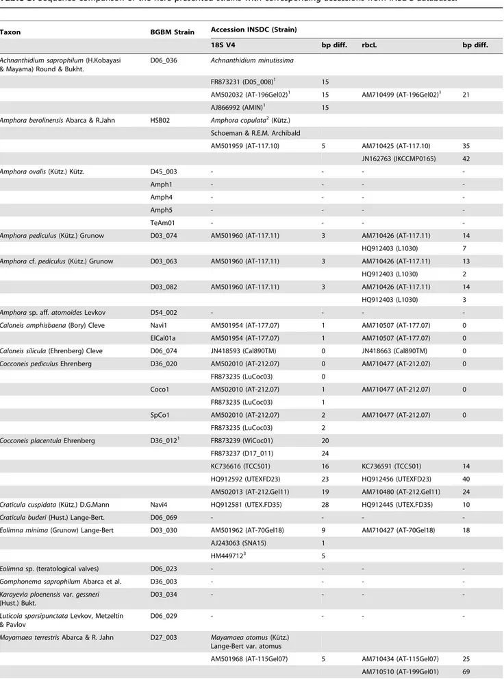
Table 3.Sequence comparison of the here presented strains with corresponding accessions from INSDC databases.

Taxon BGBM Strain Accession INSDC (Strain)

18S V4 bp diff. rbcL bp diff.

Achnanthidium saprophilum(H.Kobayasi & Mayama) Round & Bukht.

D06_036 Achnanthidium minutissima

FR873231 (D05_008)1 ₁₅

AM502032 (AT-196Gel02)1 ₁₅ _{AM710499 (AT-196Gel02)}1 ₂₁

AJ866992 (AMIN)1 ₁₅

Amphora berolinensisAbarca & R.Jahn HSB02 Amphora copulata2_(Ku¨tz.)

Schoeman & R.E.M. Archibald

AM501959 (AT-117.10) 5 AM710425 (AT-117.10) 35

JN162763 (IKCCMP0165) 42

Amphora ovalis(Ku¨tz.) Ku¨tz. D45_003 - - -

-Amph1 - - -

-Amph4 - - -

-Amph5 - - -

-TeAm01 - - -

-Amphora pediculus(Ku¨tz.) Grunow D03_074 AM501960 (AT-117.11) 3 AM710426 (AT-117.11) 14

HQ912403 (L1030) 7

Amphoracf.pediculus(Ku¨tz.) Grunow D03_063 AM501960 (AT-117.11) 3 AM710426 (AT-117.11) 13

HQ912403 (L1030) 2

D03_082 AM501960 (AT-117.11) 3 AM710426 (AT-117.11) 14

HQ912403 (L1030) 3

Amphorasp. aff.atomoidesLevkov D54_002 - - -

-Caloneis amphisbaena(Bory) Cleve Navi1 AM501954 (AT-177.07) 1 AM710507 (AT-177.07) 0

ElCal01a AM501954 (AT-177.07) 1 AM710507 (AT-177.07) 0

Caloneis silicula(Ehrenberg) Cleve D06_074 JN418593 (Cal890TM) 0 JN418663 (Cal890TM) 0

Cocconeis pediculusEhrenberg D36_020 AM502010 (AT-212.07) 0 AM710477 (AT-212.07) 0

FR873235 (LuCoc03) 0

Coco1 AM502010 (AT-212.07) 1 AM710477 (AT-212.07) 0

FR873235 (LuCoc03) 1

SpCo1 AM502010 (AT-212.07) 2 AM710477 (AT-212.07) 0

FR873235 (LuCoc03) 2

Cocconeis placentulaEhrenberg D36_0121 _{FR873239 (WiCoc01)} ₂₀

FR873237 (D17_011) 24

KC736616 (TCC501) 16 KC736591 (TCC501) 14

HQ912592 (UTEXFD23) 23 HQ912456 (UTEXFD23) 40

AM502013 (AT-212.Gel11) 19 AM710480 (AT-212.Gel11) 24

Craticula cuspidata(Ku¨tz.) D.G.Mann Navi4 HQ912581 (UTEX.FD35) 28 HQ912445 (UTEX.FD35) 10

Craticula buderi(Hust.) Lange-Bert. D06_069 - - -

-Eolimna minima(Grunow) Lange-Bert D03_030 AM501962 (AT-70Gel18) 9 AM710427 (AT-70Gel18) 18

AJ243063 (SNA15) 1

HM4497123 ₅

Eolimnasp. (teratological valves) D06_023 - - -

-Gomphonema saprophilumAbarca et al. D36_003 - - -

-Karayevia ploenensisvar.gessneri (Hust.) Bukt.

D03_034 - - -

-Luticola sparsipunctataLevkov, Metzeltin & Pavlov

D06_029 - - -

-Mayamaea terrestrisAbarca & R. Jahn D27_003 Mayamaea atomus(Ku¨tz.) Lange-Bert var. atomus

AM501968 (AT-115Gel07) 5 AM710434 (AT-115Gel07) 25

AM710510 (AT-199Gel01) 69 Taxonomic Reference Libraries for Environmental Barcoding of Diatoms

(11)

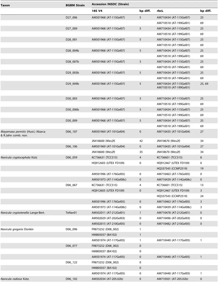
Table 3.Cont.

D27_006 AM501968 (AT-115Gel07) 5 AM710434 (AT-115Gel07) 25

AM710510 (AT-199Gel01) 69

D28_004b AM501968 (AT-115Gel07) 5 AM710434 (AT-115Gel07) 25

AM710510 (AT-199Gel01) 69

D29_009b AM501968 (AT-115Gel07) 5 AM710434 (AT-115Gel07) AM710510 (AT-199Gel01)

25, 69

AM710510 (AT-199Gel01) 69

Mayamaea permitis(Hust.) Abarca & R.Jahn comb. nov.

JN418600 (Wes2f) 42 JN418670 (Wes2f) 34

JN418600 (Wes2f) 35 JN418670 (Wes2f) 34

Navicula cryptocephalaKu¨tz D06_059 KC736631 (TCC515) 4 KC736601 (TCC515) 8

HQ912603 (UTEX FD109) 0 HQ912467 (UTEX FD109) 0

HQ337543 (CCMP2519) 19

AM501996 (AT-176Gel05) 0 AM710463 (AT-176Gel05) 0

AM501973 (AT-114Gel08c) 0 AM710439 (AT-114Gel08c) 0

D06_067 KC736631 (TCC515) 4 KC736601 (TCC515) 13

HQ912603 (UTEX FD109) 0 HQ912467 (UTEX FD109) 3

HQ337543 (CCMP2519) 24

AM501996 (AT-176Gel05) 0 AM710463 (AT-176Gel05) 3

AM501973 (AT-114Gel08c) 0 AM710439 (AT-114Gel08c) 3

Navicula cryptotenellaLange-Bert. TeNav01 AM502011 (AT-212Gel01) 1 AM710478 (AT-212Gel01) 0

AM502029 (AT-202Gel03) 0 AM710496 (AT-202Gel03) 0

AM502015 (AT-210Gel05) 0 AM710482 (AT-210Gel05) 0

Navicula gregariaDonkin D06_096 FR873252 (D08_002) 1

HM805037 (BA102) 1

AM501974 (AT-117Gel05) 1 AM710440 (AT-117Gel05) 1

D06_077 FR873252 (D08_002) 0

HM805037 (BA102) 0

AM501974 (AT-117Gel05) 0 AM710440 (AT-117Gel05) 1

D06_122 FR873252 (D08_002) 0

HM805037 (BA102) 0

AM501974 (AT-117Gel05) 0 AM710440 (AT-117Gel05) 1

Navicula radiosaKu¨tz. D06_102 AM502034 (AT-205.02b) 0 AM710501 (AT-205.02b) 0

(12)

recently transferred to the genusHalamphora[37]; these taxa and also the two INSDC accessions listed as Halamphora in the (numbers AB754832, AB754833;) are forming a loose cluster in

the upper part of the 18S V4 tree (Fig. 7a). TherbcL data set supports an independent clade for the taxa of the genus Halamphora (Amphora coffeaeformis, Amphora normannii,

Am-Table 3.Cont.

AM502027 (AT-200.04) 0 AM710494 (AT-200.04) 0

AM501972 (AT-114Gel06) 0 AM710438 (AT-114Gel06) 0

Navicula rhynchotellaLange-Bert. D06_093 - - -

-D06_095 - - -

-D06_087 - - -

-D06_083 - - -

-Navicula slesvicensisGrunow D06_038 - - -

-Navicula tripunctata(O.F.Mu¨ll.) Bory D03_093 AM502028 (AT-202.01) 0 AM710495 (AT-202.01) 0

D03_139 AM502028 (AT-202.01) 0 AM710495 (AT-202.01) 0

Navi5 AM502028 (AT-202.01) 0 AM710495 (AT-202.01) 0

Pinnularia neomajorKrammer Pinn1 JN418585 (Corsea2) 0 JN418655 (Corsea2) 0

JN418571 (Tor1a) 31 JN418641 (Tor1a) 15

PinnB JN418585 (Corsea2) 0 JN418655 (Corsea2) 0, 15

JN418571 (Tor1a) 31 JN418641 (Tor1a)

Pinnularia viridiformisKrammer Pinn2 JN418589 (Pin870MG) 22 JN418659 (Pin870MG) 19

JN418574 (Enc2a) 26 JN418644 (Enc2a) 24

AM501985 (AT-70.10) 9 AM710451 (AT-70.10) 5

AM743108 (L1716) 97

ElPin01 JN418589 (Pin870MG) 22 JN418659 (Pin870MG) 19

JN418574 (Enc2a) 26 JN418644 (Enc2a) 24

AM501985 (AT-70.10) 9 AM710451 (AT-70.10) 5

AM743108 (L1716) 97

Pinnulariasp. Navi2 - - -

-Pinnulariasp. PinnC - - -

-Planothidium frequentissimum(Lange-Bert.) Lange-Bert.

D06_138 - - -

-D06_139 - - -

-Planothidium caputiumR.Jahn & Abarca sp. nov. D06_014 - - -

-D06_113 - - -

-Planothidium lanceolatum(Bre´b. ex Ku¨tz.) Lange-Bert.

D06_047 AJ535189 (L1249) 2 JQ610173 (LCR-S2-1-1) 17

Sellaphora pupula(Ku¨tz.) Mereschk. D06_060 EF151973 (Bel2) 1 EF143266 (Bel2) 0

EF151983 (Aus4) 1 EF143317 (Aus4) 15

D06_110 EF151973 (Bel2) 1 EF143266 (Bel2) 0

EF151983 (Aus4) 1 EF143317 (Aus4) 15

Sellaphora seminulum(Grunow) D.G.Mann D06_006 EF151967 (TM37) 0 EF143280 (TM37) 32

KC736642 (TCC461) 22 KC736613 (TCC461) 16

Stauroneis phoenicenteron(Nitzsch.) Ehrenb. Stau1 AM502031 (AT-182.07) 0 AM710498 (AT-182.07) 0

AM501987 (AT-117.04) 2 AM710453 (AT-117.04) 0

Stauroneis schmidiaeR.Jahn & Abarca sp. nov. D28_002 - - -

-D28_008 - - -

-Basepair differences (bp diff.) for each taxon and strain number specified for both markers 18S V4 andrbcL. – denotes missing representative for taxon in INSDC databases (accessed July 2013).

1

Achnanthidium minutissimum(Ku¨tzing) Czarnecki.

2_{new name for the taxon formerly identified as}_{Amphora libyca}_Ehrenberg. 3_as_{Navicula minima.}

doi:10.1371/journal.pone.0108793.t003

(13)

(14)

phora montana; 0.97 BS; Fig. 7b). However, within the Halam-phoraclade the strains identified asAmphora coffaeaformisare not monophyletic (Fig. 7b).

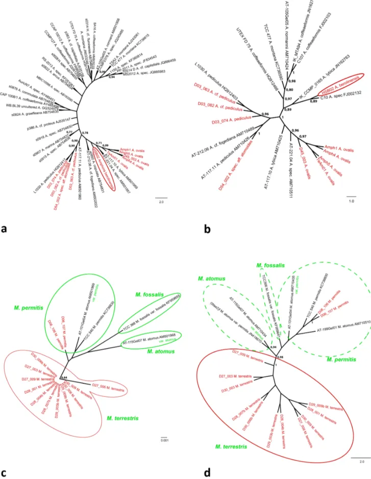
The trees for the genusMayamaeaincluding all available data from INSDC databases are given in Fig. 7c (18S V4) and Fig. 7d (rbcL). All strains identified asMayamaea terrestrisare forming an independent clade in both trees (0.84 BS in 18S V4, 1.00 BS in rbcL; Fig. 7c, 7d). The strains D06_106 and D06_107 represent-ing Mayamaea permitis (Syn.: Mayamaea atomus var. permitis) cluster together in one clade (in rbcL 1.00 BS), however other strains named either Mayamaea atomus, Mayamaea permitis or Mayamaea atomusvar.permitisshow no clear pattern according to their names provided in the INSDC databases (Fig. 7c, 7d).

The trees for the genus Planothidium including all available data from INSDC databases are given in Fig. 8a (18S V4) and Fig. 8b (rbcL). 18S V4 supports three independent clades for the three including Planothidium taxa; namely Planothidium capu-tium, Planothidium frequentissimum and Planothidium lanceola-tum(each taxon supported by 1.00 BS; Fig. 8a). Strain LCR-S18-1-1 (INSDC accession number JQ610164), listed in the INSDC databases as Planothidium sp., sits on another branch (Fig. 8a). The topology derived fromrbcL sequences gives one clade (0.97 BS) forPlanothidium caputiumand strain LCR-S18-1-1 (INSDC accession number JQ610172) plus a second clade for a mono-phyletic groupPlanothidium frequentissimum (0.92 BS; Fig. 8b). The strains identified asPlanothidium lanceolatumdo not form an independent clade in therbcL analysis (Fig. 8b).

The trees for the genusStauroneisincluding all available data from INSDC databases are given in Fig. 8c (18S V4) and Fig. 8d (rbcL). The Stauroneis schmidiae strains (D28_002, D28_008) cluster in one clade, which is sister to the strain UTEX FD 51 (INSDC accession numbers HQ912579 (18S V4) and HQ912443 (rbcL)) in both analyses (1.00 BS; Fig. 8c, 8d). The strain Stau1 is identified asStauroneis phoenicenteronand forms a monophyletic clade (1.00 BS for both markers) with all the other accessions with this name available from the INSDC databases (AT-18.207 (INSDC accession numbers AM502031 (18S V4) and AM710498 (rbcL)) and AT-11.704 (INSDC accession numbers AM501987 (18S V4) and AM710453 (rbcL))). The other taxa available from the INSDC databases also cluster taxonomically consistent, however there are difference in the overall topology recovered from 18S V4 respectivelyrbcL sequences (Fig. 8c, 8d).

Nomenclatural and taxonomical consequences

Two new taxa were first discovered by morphological means namely Amphora berolinensis and Stauroneis schmidiae. The analysis of molecular data suggested the existence of two more previously undetected taxa that could later be also

morphologi-cally confirmed (Mayamaea terrestris, Planothidium caputium). For yet another two taxa morphological data is incomplete (teratological outline, micro-morphological data missing) but the molecular data show that they both are different from an identified taxon in this genus; these strains are named sp. (Amphorasp. aff. atomoides); in one case we used the term cf. (Amphoracf.pediculus) to show that it is closely related to a known taxon.

Amphoracf.pediculus

The strains D03_063 & D03_082are morphologically very similar to our Amphora pediculus D03_074 but have double areolae in each ventral stria and not only a single elongated areola likeA. pediculus. The specimens of these strains have a similar valve outline asA. indistincta, but in SEM the differences are more distinct because in A. indistincta the width of the central and dorsal side is almost equal and the striae are composed of elongated areolae.

Amphorasp. aff.atomoidesLevkov

The strain D54_002has a valve semi elliptical with arched dorsal margin, concave ventral margin and narrowly rounded valve ends. Valve length is 10–12.4mm, breadth 4.6–5mm. The central area on dorsal side is a rectangular fascia almost extending to the dorsal margin; on the ventral side the much broader fascia is expanding towards the valve margin. Raphe branches linear, filiform. Proximal raphe endings straight, distal raphe endings ventrally deflected. Dorsal striae radiate throughout, 16 in 10mm. This species closely resemblesA. atomoidesbut differences can be observed in the shape of the central area and valve breadth (7– 11mm inA. atomoides). InA. atomoidesthe central area on the dorsal side is small or absent not extending to the valve margin, contrary to our Amphora sp. aff.atomoideswhere the central area presents a rectangular fascia almost extending to the dorsal margin. D54_002 also resemblesA. pediculuswith respect to its valve shape and size. However D54_002 can be differentiated by the valve width (A. pediculus is narrower with 2.5–4mm) the central area (A pediculushas a distal raphe dorsally deflected and a central area with a rectangular facia, extended to the dorsal valve margin) and the stria density (A. pediculushas more striae 18–24/ 10mm). D54_002 can also be differentiated fromA. minutissima by the shape of valve apices (ventrally bent inA. minutissima). Additional observations of more specimens by SEM would be necessary to establish the proper identity of this population from Heiligensee, Berlin.

Four taxa in the genera Amphora, Mayamaea, Planothidium, andStauroneisdo not fall within the description of any previously known taxa and are therefore described here as new.

Figure 3. LM photos of individual valves from strains.Fig. 3.1.Achnanthidium saprophilum(H.Kobayasi & Mayama) Round & Bukht., Strain D06_036. Fig. 3.2.–3.Planothidium frequentissimum(Lange-Bert.) Lange-Bert., Strain D06_139. Fig. 3.4.–5.Planothidium lanceolatum(Bre´b. ex Ku¨tz.) Lange-Bert., Strain D06_047. Fig. 3.6.Karayevia ploenensisvar.gessneri(Hust.) Bukt., Strain D03_034. Fig. 3.7.Luticola sparsipunctataLevkov, Metzeltin & Pavlov, Strain D06_029. Fig. 3.8.Amphora pediculus(Ku¨tz.) Grunow, Strain D03_074. Fig. 3.9.Amphorasp. aff.atomoidesLevkov, strain D54_002. Fig. 3.10.Amphoracf.pediculus(Ku¨tz.) Grunow, Strain D03_082. Fig. 3.11. Amphora ovalis(Ku¨tz.) Ku¨tz., Strain Amph4. Fig. 3.12.Cocconeis pediculus

Ehrenberg, Epitype-Strain D36_020. Fig. 3.13.Cocconeis placentulaEhrenberg, Epitype-Strain D36_012. Fig. 3.14.Sellaphora seminulum(Grunow) D.G.Mann, Strain D06_006. Fig. 3.15.Eolimna minima(Grunow) Lange-Bert., Strain D03_030. Fig. 3.16.Sellaphora pupula(Ku¨tz.) Mereschk., Strain D06_060. Fig. 3.17.–18.Mayamaea permitis(Hust.) Bruder & Medlin, Strain D06_106. Fig. 3.19.Caloneis amphisbaena(Bory) Cleve, Strain Navi1. Fig. 3.20.Navicula tripunctata(O.F.Mu¨ll.) Bory, Strain D03_139. Fig. 3.21.Navicula rhynchotellaLange-Bert., Strain D06_093. Fig. 3.22.Navicula radiosa

Ku¨tz., Strain D06_102. Fig. 3.23.Craticula cuspidata(Ku¨tz.) D.G.Mann, Strain Navi4. Fig. 3.24.Navicula gregariaDonkin, Strain D06_122. Fig. 3.25.

Craticula buderi(Hust.) Lange-Bert., Strain D06_069. Fig. 3.26.Navicula cryptocephalaKu¨tz., Strain D06_059. Fig. 3.27.Navicula slesvicensisGrunow,

Strain D06_038. Fig. 3.28.Stauroneis phoenicenteron(Nitzsch) Ehrenb., Strain Stau1. Fig. 3.29.Pinnularia neomajorKrammer, Strain PinnB. Fig. 3.30.

Pinnulariasp., Strain PinnC. Fig. 3.31.Pinnularia viridiformisKrammer, Strain Pinn2. Fig. 3.32.Pinnularia viridiformisKrammer, Strain ElPin01. Fig. 3.33.

Pinnulariasp., Strain Navi2. Fig. 3.34.Gomphonema saprophilum(Lange-Bert. & Reichardt) N.Abarca, R.Jahn, J. Zimmermann & Enke, Strain D36_003.

Scale bar represents 10mm.

(15)

(16)

Amphora berolinensisN.Abarca & R.Jahn (Figs. 4.1a–i) Holotype: B 40 0040871 from strain HSBO2; the holotype is represented by Fig. 4.1d.

Type locality: Germany, Berlin, Heiligensee, N 52.60394uE 13.21499uleg. and isolated by O. Skibbe, August 2011.

Amphora berolinensisdiffers fromA. copulata(Ku¨tzing) Schoe-man & Archibald because the latter has bigger valves (19–42mm length, 5–7.5mm breadth). In SEM the differences are more distinct. Differences can be observed in the shape of the central area (bordered by striae close to the valve margin inA. copulata), the raphe (biarcuate inA. copulata) and the morphology of the dorsal striae (crossed by longitudinal bars in A. copulata). A. berolinensealso differs fromA. neglectiformisLevkov & Edlund by the larger valves of the later (18–53mm length, 5–7mm breadth) and the ventral striae which are composed of two areolae inA. neglictiformisnear the valve ends.

The valves ofAmphora berolinensisare lanceolate to semi-elliptical, with smoothly arched dorsal margin and straight to slightly concave ventral margin, valve ends rounded. Valve length is 9.5–18.9mm, breadth 4.7–5.2mm. Axial area is narrow, slightly arched. The central area on the dorsal side has a rectangular fascia extending to the dorsal margin; on the ventral side the fascia is wider expanding towards the valve margin. Raphe is filiform and more or less straight, in some valves the proximal raphe endings are straight, in others they are dorsally bent and the distal raphe endings are straight and in some valves they are ventrally bent. Dorsal striae are coarsely punctated and radiate throughout, 12– 14 in 10mm. Ventrally striae are radiate, composed of one areola. Amphora copulata (Ku¨tz.) Schoeman & R.E.M. Archibald (concept syn. Amphora libyca Ehrenberg, sensu post auct.) is morphologically the closest fit toAmphora berolinensis, the latter forms a distinctly different clade according to both 18S V4 and rbcL (Fig. 7a, 7b). The sequence difference to strain AT-117.10 belonging toAmphora libycasensu post auct. is e.g. 5 bp for 18S V4 and 35 bp forrbcL.

Mayamaea terrestrisN.Abarca & R.Jahn sp. nov. (Fig. 4.2a–g)

Holotype: B 40 0040847 from strain D29_009b; the holotype is represented by Fig. 4.2e.

Type locality: Germany, Berlin-Dahlem, agricultural soil, N 52.460833uE 13.296944u, leg. L. Buhr, 21 April 2004, cultures isolated by J. Bansemer.

Mayamaea terrestrisdiffers fromMayamaea atomusvar.atomus [47] because the latter is longer and wider and has less striae (8.5– 13mm length, 4–5.5mm breadth, 19–22/10mm striae). Also the molecular data differ fromMayamaea atomusvar.atomusentries in the INSDC databases in 5 bp for 18S V4 and 25 bp forrbcL of strain AT-115Gel07 and even in 69 bp for rbcL of strain AT-199Gel01 (AM710510) [48].

The valves of Mayamaea terrestris are narrow linear-elipical, ends obtusely rounded. Valve length is 7–8.7mm, breadth 3– 4.5mm. Striae are radiate throughout, 22–24 (–26) in 10mm with c. 50 areolae in 10mm. Raphe is filiform, the two branches are gently arcuate with distinct central pores. Axial area is slightly broad, widening lanceolately towards the middle of the valve. Central raphe ends expanded by depressions around the central

pores and deflected, while the ends of the terminal raphe fissures are deflected to the opposite side.

This new species lives in soil; this is signified by the epithet name.

10 further strains (D27_003 & D27_006 & D27_009 & D28_001 & D28_004b & D28_007b & D29_003b & D30_003 & D30_006b & D30_009) have only low sequence differences for 18S V4 andrbcL (Appendix S2) and form a clade clearly different from all the other availableMayamaeastrains (Fig. 7c, 7d).

Planothidium caputiumJ.Zimmermann & R.Jahn sp. nov. (Fig. 4.3a–h)

Holotype: B 40 0040871; strain D06_014; the holotype is represented by Fig. 4.3f.

Type locality: Germany, Berlin, small river Wuhle, N 52.52079uE 13.57781u, leg. O. Skibbe, 21 April 2004, cultures isolated by J. Bansemer.

Morphologically,Planothidium caputiumhas a similar outline asPlanothidium lanceolatumbut differs from it by a hood over the depression on the rapheless valve as inP. frequentissimum. The difference toP. frequentissimumlies in the form and size of the hood; which is bigger, longer and wider inP. caputiumthan inP. frequentissimumand the hood has a wider opening; this results in a line-like instead of a horse shoe appearance when focusing through the hood. The uncorrected p-distances show that Planothidium caputiumsequences differ at least 2.4% (18S V4) respectively 2% (rbcL) from Planothidium frequentissimum, and 6% (18S V4) respectively 4% (rbcL) fromPlanothidium lanceolatum(Appendix S2), this is also represented in the trees including all available Planothidiumstrains (Fig. 8a, 8b).

Valves are elliptical to elliptic-lanceolate, with rounded apices. Valve length is 20–22.9mm, breadth 5.5–6.4mm. The striae are radiate on both valves, becoming more radiate towards the apices, with 13–14 in 10mm. Striae are multiseriate with three to five rows of areolae per stria. The axial area is narrow and linear to lanceolate in both valves. A weak central area on the raphe valve and a horseshoe-shaped collar on one side of the rapheless valve which by focusing in LM another line less arched can be recognized (see also Straub 1990 [49]).

Also strain D06_113 belongs to this species.

Stauroneis schmidiaeR.Jahn & N.Abarca sp. nov. (Fig. 4.4a–h)

Holotype: B 40 0040883 from strain D28_008; the holotype is represented by Fig. 4.4f.

Type locality: Germany, Berlin-Dahlem, agricultural soil, N 52.460833uE 13.296944u, leg. L. Buhr, 21 April 2004, cultures isolated by J. Bansemer.

Morphologically,Stauroneis schmidiae differs fromStauroneis borrichii(Petersen) Lund, which has a similar valve outline but with protracted ends, because the latter is shorter and more slender and has more striae (18–25mm length, 4.0–5.0 breadth, 20–22 striae and 25–28 punctae per 10mm (see Van de Vijver et al 2004) and fromStauroneis pseudomuriella Van de Vijver & Lange-Bert. (2004) [50] which has similar morphometrics as our new species but more striae (21–42mm length, 5–6.5mm breadth,

Figure 4. SEM and LM photos of the newly described species.Figs. 4.1a–i.Amphora berolinensisN.Abarca & R. Jahn sp. nov., Strain HSB02; Fig. 4.1d–i. Holotype B 40 0040823. Figs. 4.2a–g.Mayamaea terrestrisN.Abarca et R.Jahn sp. nov., Strain D29_009b; Fig. 4.2d–g. Holotype B 40 0040847. Figs. 4.3a–h.Planothidium caputiumJ.Zimmermann & R.Jahn sp. nov., Strain D06_014; Fig. 4.3e–h Holotype B 40 0040871. Fig. 4.4a–h.Stauroneis

schmidiaeR.Jahn & N.Abarca sp. nov., Strain D28_008; Fig. 4.4f–h. Holotype B 40 0040882.

(17)

20–22 striae and 25 punctae per 10mm) but this species has no pseudosepta.

Valves are linear-lanceolate with very slightly rounded non-protracted ends. Valve length is 27–28.2mm, breadth 5.5–6mm.

Striae are radiate throughout the entire valve, 15–18 in 10mm. Puncta of the striae are discernible in LM and are 24–28 in 10mm. Pseudosepta present.

Also strain D28_002 belongs to this species.

Figure 5. Chart giving classes of base pair (bp) differences for both markers (18S V4,rbcL) between here presented molecular data and corresponding data from INSDC databases.Inferred from data in Table 3.

(18)

Compared to the other availableStauroneisstrainsStauroneis schmidiaeclusters independently for both markers (Fig. 8c, 8d).

This species is named in honor of Prof. Dr. AnnaMaria Schmid who was an inspiring diatom teacher to Regine Jahn.

Discussion

The 37 naviculoid diatom taxa, of which reference barcodes are published here, represent only about 7% of the total diatom flora

which is 14% of the naviculoid taxa recorded for Berlin waters (539 taxa, see [31]). Nevertheless, it is a first milestone in characterising diatoms not only by morphological but also by molecular means, which represents the start of a taxonomic reference library for diatoms.

Identification via DNA sequences is an important tool, especially in microorganisms. Many of the large scale environ-mental DNA barcoding studies in protists so far rely on higher taxonomic levels of families and above; only rarely they reach a

Figure 6. Neighbour Joining Tree (10 000 bootstrap replicates) derived from concatenated dataset (18S V4,rbcL) including all sequences from this study.All bootstrap support values given above branches.

(19)

Figure 7. Neighbour Joining Tree (10 000 bootstrap replicates) including all sequences available from the INSDC databases for genusAmphora(a) 18S V4, (b)rbcL as well asMayamaea(c) 18S V4, (d)rbcL.Bootstrap support values.0.75 given at nodes. Red indicates data from new species, green information and conlusions derived from data in the AlgaTerra Information System [30].

(20)

(21)

resolution at genus level. In diatoms, assignment to genus level is unproblematic [51,52]. Even identification to the species level is possible, but strongly depends on the quality of the reference database [52–58]. We here tested the taxonomic consistency of naviculoid diatom taxa at the species level by comparing our identified sequences with the published sequences in the reposi-tories of the INSDC. We found that the taxonomic assignment in INSDC is currently unsatisfying, because it is often erroneous. In the data of the two commonly used DNA barcoding markers for diatoms 18S V4 and rbcL we analysed, we found that forrbcL 26% for the sequences listed under the same name as our strains more than 15 bp sequence difference were recorded (Fig. 5b); for 18S V4 this was 12% (Fig. 5a). For the 800 bp longrbcL fragment 15 bp difference amounts to roughly 2% sequence difference, in the shorter (400 bp) 18S V4 fragment 15 bp difference correlates to even 4%. The relatively high percentage of differences in these short DNA fragments suggests that the sequences belong to a different taxon. This implies morphology-related misidentification, mislabelling or cross-contamination. There are an additional 16% (rbcL, Fig. 5b) respectively 5% (18S V4, Fig. 5a) of the sequences where sequences with the same taxon name showed differences between 6 and 15 bp, here it is unclear whether these strains belong to a different taxon of a closely related cryptic species or whether they reflect natural intraspecific variation. Furthermore, we found that in 4% (rbcL, Fig. 5b) respectively 15% (18S V4, Fig. 5a) of the cases, identical sequences in the repositories of the INSDC were annotated with a different taxon name than the strains of this study. These sequences therefore provide an erroneous identification. In summary, the unevaluated use of information deposited in the INSDC leads to wrong identifications in at least 30% of the cases; in only about 20% of our cases, the identifications coincided unambiguously.

Unfortunately, in most cases it is not possible to trace the DNA sequence to the specimen from which it originated and, because of lacking voucher specimens, taxonomic evaluation is not possible; hence there are no means to verify whether a faulty taxon assignment had occurred or an interesting biological phenomenon. Therefore such sequences are of no future use and valuable information is lost to science. Assessment of diatom community composition through environmental DNA barcoding could greatly benefit from better documented reference libraries, especially because biodiversity in general should be evaluated at least on the species level [59].

Furthermore, the linkage between historically and morpholog-ically described taxa and molecular sequences is not very strong. A possible threat is that two independent data clouds might develop [60]: one including large amounts of molecular data from environmental sequencing, the other species specific data (e.g. paleontological and recent distribution, ecology, phylogeny) linked to morphological descriptions. For organism groups where next to no morphology based data exist (e.g. many groups of bacteria), there is little harm if the information in the two clouds cannot be correlated. However, in groups like diatoms, where two centuries of data collection linked to morphologically described species exists, it would be a waste of painfully acquired data not to link these two groups of data. At the moment, this link would be a reference sequence that is connected to a morphological voucher (and DNA sample) deposited in a natural history collection and

therefore available for multiple testing and verification of results as well as for long-term studies.

We here define a taxonomic reference library as an entity combining molecular data – in our case DNA sequence data of two markers – with morphological documentation of important features as well as a valid name. Also environmental information on the collecting site should be provided in a standardised format. Documentation should also include the deposition of DNA in a curated repository. To ensure traceability of a name/sequence back to the specimen it originated from, morphological details important for identification should be provided in an online photographic documentation, this includes high-resolution photo-graphs giving an overview of the cell as well as details produced by electron microscopy or comparable techniques. Another special aspect for diatoms (and some other microorganism groups) is that many sequences derive from cultured clonal strains, especially if they are linked to morphological entities. Therefore, the strain number and other strain specifications are valuable information that should be presented along with the sequence.

Ideally, all the necessary information for traceable taxonomic classification should be available in a single data portal; however, at the moment there are several technological limitations to deposit and/or respectively retrieve all the information in and from one location. The Consortium for the Barcode of Life (CBOL) aims at compiling DNA barcode records in a public library (Barcoding of Life Database BOLD) [53] and even designed a Barcode Submission Tool for submitting sequences to the INSDC databases. However, this tool is limited to one marker, namely the mitochondrial cytochrome oxidase subunit I (COI) e.g. [17,61–65]. For many groups, e.g. plants [66] but also diatoms, this barcoding marker is not routinely applicable [19,21–25], albeit there are BOLD supported activities to implement alternative solutions for some organism groups e.g. [28]. On the other hand, the Barcode Submission Tool provides possibilities to at least upload a pherogram (output of sanger sequencing), but no pictures of the organisms can be stored. Therefore, this tool does not require a link to a morphological voucher (digital and physical), which would allow for subsequent taxonomic validation. Also a link to a herbarium specimen is only indirectly possible if the accession number of the specimen collection is given and the respective collection has their specimen picture online available. Although, it seems generally possible to deposit pictures and other data along with the DNA sequence in BOLD [53], unfortunately, the data deposited within BOLD is often not open access, depending on the rights given by the administrator. Also, we heard reports that data is not released to the public even if requested by the author. In conclusion it would be preferable if INSDC would extend their service, as they are the most commonly used platform to deposit sequence data [58].

Here we present our strategy on how documentation can be performed to build a comprehensive reference database for diatoms even with inconvenient IT possibilities. The here presented materials and data have been documented as follows: The physical vouchers (microscopic slides and SEM stubs) have been deposited in the Berlin Herbarium (B), the DNA in the DNA bank network of the Botanic Garden and Botanical Museum Berlin-Dahlem [39]. The data for both items are made available through The Global Genome Biodiversity Network (GGBN [67]) and The Global Biodiversity Information Facility (GBIF [68]).

Figure 8. Neighbour Joining Tree (10 000 bootstrap replicates) including all sequences available from the INSDC databases for genusPlanothidium(a) 18S V4, (b)rbcL as well asStauroneis(c) 18S V4, (d)rbcL.Bootstrap support values.0.75 given at nodes. Red indicates data from new species.

(22)

The sequences have been submitted to an INSDC database (EMBL) along with strain numbers, voucher number from the Berlin Herbarium (B) and DNA bank number. Also primer details and geo-references have been deposited there. Photographic documentation is online available from the AlgaTerra Information System [30], linked through INSDC accession number and accession number from the Berlin Herbarium. Morphological characters, cultivation details as well as sampling data of the collecting sites beyond the geo-references (e.g. ecological specifi-cations) have also been deposited in the AlgaTerra Information System [30].

A carefully documented reference sequence could be considered as something similar to a molecular type of the name of a species. Biological taxon types should be documented with a maximum amount of data, which makes it possible for every researcher to determine whether a specific specimen belongs to the concept of the designated type. In the botanical [69] and zoological [70] codes of nomenclature the basis for species description is the deposition of physical specimen. A reference sequence or reference barcode should be similarly well documented.

Biological identification systems are in constant development, therefore a continuous process of confirmation, validation and updating in relation to alpha taxonomy is required to build a compressive and accurate reference library. Protocols for data curation and revision are indispensable for new species discovery as well as taxonomic revisions. Therefore, entries in a taxonomic reference library (e.g. in an extended INSDC like system) need to be curated and updated in order to be in line with current taxonomy. However, a huge impediment for data curation by the respective author – once it is submitted – is, that there is no reward system for researchers for curating their data [71]. It has been shown, that incentives for researchers for the publication of thoroughly documented datasets similar to the publication of the conclusions drawn from these could greatly increase the motiva-tion to publish datasets [71]. Another approach would be that data curation would be carried out by professional personnel employed for this purpose or a combination of both approaches.

Not only DNA barcoding approaches would benefit from well documented and referenced molecular data but also taxonomic and phylogenetic studies of diatoms which could integrate published data more efficiently if better documentation linked to physical objects were available [72]. For example, the clusters found for the genusMayamaea, based on available 18S V4 and rbcL sequences, show low taxonomic consistency (Fig. 7c, 7d). The INSDC data suggest that there are different groups ofMayamaea (atomus var.) permitis, and within the Mayamaea atomus (var. atomus) sequences is one sequence namedMayamaea fossalisvar. fossalis (Fig. 7c, 7d, black and red). For two of the AT strains included in the Mayamaea analysis additional data is available from the AlgaTerra Information System [30] (Fig. 7c, 7d, green): (a) more taxonomic detail is given than deposited alongside the sequence in INSDC - strain AT-115Gel07 is identified as Mayamaea atomusvar. atomusand AT-101Gel04 asMayamaea atomus var. permitis - and (b) photographs with morphological details are provided. Therefore the identification of both strains could be checked and verified. Even though additional data for only two strains is available from the AlgaTerra Information System [30], this already aids in the interpretation of the trees given in Fig. 7c and 7d; especially for the tree based on 18S V4. There is a cluster ofMayamaea permitis(Syn.Mayamaea atomus var. permitis), incl. strain AT-101Gel04, and one strain (AT-115Gel07) belonging toMayamaea atomus var. atomus(Fig. 7c, green). As Mayamaea permitis (Syn. Mayamaea atomus var. permitis) has been raised to species rank due to morphological

reasons (see above), this allows the interpretation thatMayamaea fossaliscould be an independent taxon (Fig. 7c, green). For the tree based onrbcL, however, only an informed guess can be made: for two strains, namely (Wes2)f and AT-199Gel01, no additional data is available to check the identification (Fig. 7d). If it could be assumed that (Wes2)f was misidentified and AT-199Gel01 belongs to Mayamaea permitis, again four independent taxa could be assumed: Mayamaea atomus, Mayamaea fossalis, Mayamaea permitisandMayamaea terrestris. This example, particularly the different interpretation possibilities between 18S V4 and rbcL trees, clearly shows how valuable additional data can be for the interpretation of sequence based analyses.

Due to the fact that species descriptions in diatoms are based on morphology derived from microscopic pictures (of variable quality) of single, or a limited number, of valves from a presumed population in mixed samples, it is often difficult to unambiguously identify a strain. Even within a single clonal culture, morphological variation sometimes fits in parts to different species circumscrip-tions [45]. In addition, size wise clonal cultures are often at the lower end of the morphometrics of a taxon description; if cultured for too long and if no auxosporulation has taken place, diatom valves tend to lose their typical morphological features because they get smaller with each cell division. This leads to the problem how to link sequences derived from cultures to a type specimen or at least to a current species concept. If a type specimen is designated, this can be achieved e.g. through epitypification as has been done forCocconeis pediculusandC. placentula[73,74]. But in most cases, this will be done in the context of a taxonomic revision of a species group as e.g. forGomphonema saprophilum [45] and needs to be done for the two unidentified Pinnularia species of this study. For the purpose of a reference library, if no unambiguous identification seems possible, the sequence could either be designated as belonging to a certain ‘‘formenkreis’’ (taxon group) marked asaffine(e.g.Amphorasp. aff.atomoides), as not exactly fitting the original descriptions marked asconfer(e.g. Amphora cf. pediculus) [http://bionomenclature-glossary.gbif. org/], or a new taxon has to be described formally along with providing the reference sequence (e.g.Amphora berolinense). The first two options are a practical way to make re-users of the data aware of an ‘‘uncertainty level’’ concerning the taxonomic identification; this is better than providing no guidance to the species group by giving just the genus name such asAmphorasp. As we documented in this study, the marine or halophilic species ofAmphorasensu lato have been recently moved into the genus Halamphora; for a freshwater reference library, this is important ecological data. In addition, this information might become valuable for the interpretation of taxonomic discrepancies

Conclusions

As here shown exemplarily for some naviculoid diatoms, taxonomic reference libraries could serve as an online accessible and algorithmically searchable equivalent to commonly used printed identification literature. They are needed to link molecular based identification technologies with correct organism references. However, up to now searchable data bases often include large percentages of wrongly annotated sequencesand provide no possibility to trace the identification back to the respective specimen, leaving molecular based techniques often with identi-fications only to family or genus level. While for some studies this level of taxonomic depth seems to suffice (e.g. large scale biodiversity assessments), there are many studies that could profit from well documented molecular data (e.g. species inventories, monitoring, taxonomy, phylogeny). Therefore, it would be worth