Facial Expression Recognition Based on WAPA and OEPA Fastica

Humayra Binte Ali

and David M W Powers

1

Computer Science, Engineering and Mathematics School, Flinders University, Australia

Computer Science, Engineering and Mathematics School, Flinders University, Australia

A

Face is one of the most important biometric traits for its uniqueness and robustness. For this reason researchers from many diversified fields, like: security, psychology, image processing, and computer vision, started to do research on face detection as well as facial expression recognition. Subspace learning methods work very good for recognizing same facial features. Among subspace learning techniques PCA, ICA, NMF are the most prominent topics. In this work, our main focus is on Independent Component Analysis (ICA). Among several architectures of ICA, we used here FastICA and LS-ICA algorithm. We applied Fast-ICA on whole faces and on different facial parts to analyze the influence of different parts for basic facial expressions. Our extended algorithm WAPA-FastICA and OEPA-FastICA are discussed in proposed algorithm section. Locally Salient ICA is implemented on whole face by using 8x8 windows to find the more prominent facial features for facial expression. The experiment shows our proposed OEPA-FastICA and WAPA-OEPA-FastICA outperform the existing prevalent Whole-OEPA-FastICA and LS-ICA methods. .

K

ICA-Independent Component Analysis, FER-Facial Expression Recognition, OEPA-Optimal Expression specific Parts Accumulation. WAPA-Weighted All Parts Accumulation algorithm.

1.

I

This work presents a detailed examination of the use of Independent Component Analysis (ICA) for feature extraction of facial expression recognition. Mathematical and analytical investigation of ICA is given here in detail. Experimental verification of the behavior of ICA with Euclidean distance classifiers is performed here. There are several architectures to implement ICA.

2.

R

W

The work from [10] claims that the structural information of sensory inputs stays in the redundancy if the sensory input system. PCA and ICA are the most well known methods for redundancy as well as finding useful components for attaining distinguishable properties. This redundancy provides information to develop a factorial system and independent components (ICs) develop from this representation. Complex object of higher order dependencies need such representation to be encoded. Independent component representation from this sort of redundant data is a general coding strategy for the visual systems [12].

The most prominent subspace learning algorithms are PCA, ICA, NMF, LDA etc. For feature extraction from the facial expression images, most of the early FER research works extracted useful features using Principal Component Analysis (PCA). PCA is a second-order statistical method, which creates the orthogonal bases. These orthogonal bases provide the maximum variability. These variables are good source fro distinguishing features in image analysis. It is also commonly used for dimension reduction. [13] and [14] employed PCA as one of the feature extractors to solve FER with the Facial Action Coding System (FACS). We previously investigated PCA on facial expression recognition [26] and [27]. The work in [26] and [27] shows applying PCA on face parts rather whole face gives more accuracy to recognize expressions from facial image data.

3.

I

C

A

The principal component analysis (PCA) performs by the Karhunen-Loeve transformation and produces mutually uncorrelated features y (i), i=0,1…N. When the goal of image or data processing is to reduce the dimension as well as to minimize the mean-square error, Karhunen-Loeve transformation is a good solution. However, certain applications, such as the one depicted in Figure 1, the mathematical or analytical solution does not meet the expectations. In addition the more recently development of Independent Component Analysis (ICA) algorithm seeks to achieve much more complicated features than simple decorrelation of data or image analysis [Hvya 01, Como 94, Jutt 91, Hayk 00, Lee 98]. Then ICA task is defined as follows: Given the set of input samples x, determine an M x M invertible matrix W such that the entries y (i), i=0, 1…M-1, of the transformed vector

………(1)

are mutually independent. The uncorrelated ness required by PCA is less important feature than the statistical independence which independence can be implemented by ICA algorithms. Only for Gaussian random variables, this two conditions are equivalent to each other.

Seeking for statistical independence of data gives the mean of exploiting a lot more information, which lies in the higher order statistics of the data. As the example of Figure 1 shows, trying to search by analyzing information in the second order statistics only results in the least interesting, projection direction, that is, that of a0. However, a1 is the most suitable direction from the class separation point of view. Additionally, implementing ICA can unveil the higher order statistics of the data the piece of information that point’s a1 as the most suitable direction. Furthermore, the cognitive nature of human brain searches for statistically independent, by processing the (input) sensory data [7]. Barlow [8] proposes the outcome of the early processing performed in our visual cortical feature detector systems might be the result of a redundancy reduction process.

vector x is principally generated by a linear combination of statistically independent sources, which is.

……….(2)

Now the task is to exploit the information of x to define under what conditions the matrix W can be computed so as to recover the components of y from equation of (2). Usually A is mixing matrix and W is the demixing matrix.

The first condition is all independent components y (i), i=1,2…N, must be non-Gaussian and the second condition is that matrix A must be invertible. It means, in contrast to PCA, ICA is meaningful only if the random variables are non-Gaussian. And mathematically for Gaussian random variables, statistical independence is equivalent to the uncorrelatedness nature of PCA. So we have to assume that the obtained Independent Components y (i),i=1,2…N, are all Gaussian, then by using any unitary matrix, a linear transformation will be a solution [7]. On the other hand, by imposing a specific orthogonal structure onto this transformation matrix, PCA achieves a unique solution

.

4.

ICA

F

E

In a specific task like face recognition the most important information may be hidden in

higher order statistics, not just the second order statistics. An example would be phase

and amplitude spectrums. Amplitude Spectrum of an image is captured by Second-order

statistics and the phase spectrum is hidden in the higher order statistics. The phase

spectrum includes a great deal of information and also applies the human perception.

Figure 2. [PS: Phase Spectrum, AS: Amplitude Spectrum] The phase spectrum of the image 2 and Amplitude spectrum of image 1 produces the blurred image of image 2. The phase spectrum of the image 1

5.

ICA

A

5.1. ICA By Maximization Of Non Gaussianity

Non-Gaussian components are Independent [1]. Maximization of non-Gaussianity is the

simple principles for estimating ICA model. Under certain conditions, the distribution of

a sum of independent random variables have a propensity

towards a Gaussian

distribution, which is the concept of central limit theorem. By finding the right linear

combinations of the mixture variables, independent components can be estimated. The

mixing can be inverted as,

X A

S = −1 ………….………..…....(3)

Now it becomes,

AS b X b

Y = T = T ………. (4)

Here b stand for one of the rows

, but this linear combination

actually stand for

one of the independent components. But as we have no knowledge of matrix A, we

cannot determine such ‘b’, although we can find an approximate estimator. Non-

Guassianity has two different practical implementations.

5.1.1. Kurtosis

Kurtosis or the fourth order cumulant is the classical measure of non-gaussianity. It is stated by

………..…..(5) We should assume variable y to be standardized, so it can say

………..(6)

The normalized version of the fourth moment

E

{

y

}

is equal to 3 For the Gaussian case implementation. and hence

Kurt

y

Hence the kurtosis is simply a normalized version of the fourth moment. For the Gaussian case the fourth moment is equal to 3 and hence

Kurt

Y

5.1.2. Negentropy

An alternative very important measure of nonguassianity is negentropy. From mathematical analysis, the measure of non-gaussianity is zero for a Gaussian variable and always non negative for a non Gaussian random variable. We can use a slightly modified version of the definition of differential entropy as negentropy. Negentropy J is defined as

……….…….. (7)

Where is a Gaussian random variable of the same covariance matrix as .

5.2. Negentropy in terms of Kurtosis

The largest entropy among all the random variables is the Gaussian variable. The negentropy for the random variables is zeroif and only if it is a Gaussian variable, otherwise it is always positve. Moreover, the negentropy has an extra property that it is invariant for invertible transformation. But the estimation of negentropy is difficult, as it requires an estimate of the probability density function. Therefore in practice using higher order moments approximates negentropy.

……… (8)

Another approach is to generalize the higher order cumulant approximation in order to increase the robustness. Again the random variable y is assumed to be a standard variable. So that it uses expectations of general non-quadratic functions. To make it simple, we can take any two nonquadratic functions G1 & G2 such that G1 is odd & G2 is even & we obtain the following approximation [equation 9].

j

J

y

≈

K

EG

y

+

K

EG

y

−

EG

U

Where K1 & K2 are positive constant & U is standardized Gaussian variable.

6.

F

F

A

ICA

(F

ICA)

Assume that we have a collection of prewhitened random vector

x

1. Take a random initial vector w(0) of norm 1.Let

k

=

1

w

(

k

)

=

E

{

x

(

w

(

k

−

1)

x

)

}

−

3

w

(

k

−

1)

x

3. Divide

w

(

k

)

w

(

k

)

w

(

k

−

1)

k

=

k

+

1

Otherwise, output the vector

w

(

k

)

6.1. Performance Index

A well-known formula for measuring the separation performance is Performance Index (PI)[1] which is defined as

= = − − = m i n

j j i j j i A A n m A PI

1 1 ,

, ) 1 ] [ max ] [ ( ) 1 ( 1 ) ( ………(10)

Where [A]i,j is the (i,j)th-element of the matrix [A]. As because, the knowledge of the mixing matrix [A] is required, the smaller value of PI usually mentions the better performance evaluation for experimental settings.

6.2. Proposed Algorithm

As pre-processing we did differentiation on whole set of images. Then we applied ICA on whole faces and on different facial parts, which hold the prominent characteristics for expression detection. In [26 & 27], we implemented PCA on whole and part based faces. In this paper we implemented ICA incorporating (i) Weighted All Parts Accumulation (WAPA) algorithm and (ii) Optimal Expression-specific Parts Accumulation (OEPA). We consider four parts left eye, right eye, mouth and nose and we found better results.

First Approach:

Weighted All Parts Accumulation (WAPA) algorithm

Step: Apply the relevant equation to identify an expression

--Ehap = W1.LEhap + W2.REhap + W3.Nhap + W4.Mhap --Eang = W1.LEang + W2.REang + W3.Nang + W4.Mang --Edis = W1.LEdis + W2.REdis + W3.Ndis + W4.Mdis --Efear = W1.LEfear + W2.REfear + W3.Nfear + W4.Mfear --Esur = W1.LEsur + W2.REsur + W3.Nsur + W4.Msur --Esad = W1.LEsad + W2.REsad + W3.Nsad + W4.Msad

LE=Left eye, RE=Right Eye, M=Mouth, N=Nose In these equations, we calculate the weighted average of the four parts of faces, eye (left, right), nose and mouth.

Second approach:

Algorithm of Optimal Expression-specific Parts Accumulation (OEPA)

Initialization:

Evaluation:

• --Step 1: Assume I = [i1, i2, i3, i4] is the vector of different segments of facial region, like: both eyes, mouth and nose.

• --Step 2: Evaluate fitness f (I (i)) representing the accuracy of detection based on a particular instance of I (i), where i = 1to 4.

• --Step 3: Assume E = [e1, e2, e3, e4, e5, e6] is the vector for six basic emotions, like: happy, sad, disgust, anger, fear and surprise. For each expression E (j), we need to run step 4 and step 5, where j = 1to 6.

• --Step 4: Assume P = I (i) for each region, where i = 1to 4 and

K1 = max (f (P)), accuracy value for detection of expression E(j).

K2 = max (f (P1 + P2)), accuracy value for detection of region P1 and P2 for the expression E(j), where P1 = P2.

K3 = max (f (P1 + P2 + P3) =accuracy value for detection of P1, P2 and P3 expression where P1 = P2 = P3.

K4=max (f(P1+P2+P3+P4)=accuracy value for detection of P1,P2,P3 and P4 expression where P1 = P2 = P3 = P4.

• --Step 5: Get the facial region

P

for which L = max (Ki)| here L is the final accuracy value for the particular expression.

7.

L

S

ICA

The Locally Salient Independent Component Analysis (LS-ICA) is an extension of ICA in terms of analyzing the region based local basis images. In terms of facial expression detection this method outperforms simple ICA due to its ability to identify local distortions more accurately. It needs two-step to compute the LS-ICA. First thing is to create component based local basis images based on ICA architecture and then order the obtained basis images in the order of class separability for achieving good recognition.

The LS-ICA method imposes additional localization constraint in the process of the kurtosis maximization. Thus it creates component based local basis images. Each iterative solution step is weighted. And it becomes sparser by only emphasizing larger pixel values. This sparsification contributes to localization. Let V be a solution vector at an iteration step, we can define a weighted solution, W where Wi Vi Vi

β

| ) ( |

= and W = W /|| W ||. > 1 is a small constant. The kurtosis is maximized in terms of W (weighted solution) instead of V as in equation 11.

2 2 4

) ) ( ( 3 ) ( )

(w E W E b

Kurt = − ………(11)

3 1

) ) (

(V S t Q

Q V E

S i i T

t β β

=

+ ………… ……… (12)

Here (in equation 12) S is a separating vector and Q contains whitened image matrix. Then the resulting basis image is ( )i.

T i i

Q S V

W = β Then according to the algorithm LS- ICA basis images are created from the ICA basis images selected in the decreasing order of the class

separability P [11], where

within between P

Ω Ω

= _{. Thus both dimensional reduction and good}

recognition performance can be achieved. The output basis images contain localized facial features that are discriminant for change of facial expression recognition.

8.

D

For experimental purpose we benchmark our results on Cohn Kanade Facial Expession dataset.e Nearly 2000 image sequences from over 200 subjects are in this dataset. All the expression dataset maintain a sequence from neutral to highest expressive grace. We took two highest graced expressive image of each subject. As we took 100 subjects, so the total image becomes 1200. 100 subject x 6 different expression x 2 of each expression. SO it becomes 100 x 6 x 2=1200. There is a significant variation of age group, sex and ethnicity. As mentioned in original dataset copyright, two Panasonic WV3230 cameras, each connected to a Panasonic S-VHS AG-7500 video recorder with a Horita synchronized time-code generator, has been used to capture the facial expressions. Although they captured frontal image and also 30 degree rotated images, for this study we only use the frontal images. Subjects display six basic emotions, happiness, sad, anger, fear, disgust and surprise. The way of performing the action is instructed by an experimenter. The experimenter is trained about the facial action coding system (FACS). Each expression starts from neutral face to the highest peak of any expression. We use the two highest grace from every expression. So it reduces the total number of used images.

The following figure (Figure 3) shows a portion of the dataset of our experiment. The first row is the frontal faces from CK dataset. Second, third, fourth and fifth rows show mouth, left eye, and right eye and nose respectively.

Figure 3. Original Dataset from CK database and the four parts of every image obtained from our algorithm and used as data.

9.

E

S

9.1. Face and Facial Parts Detection

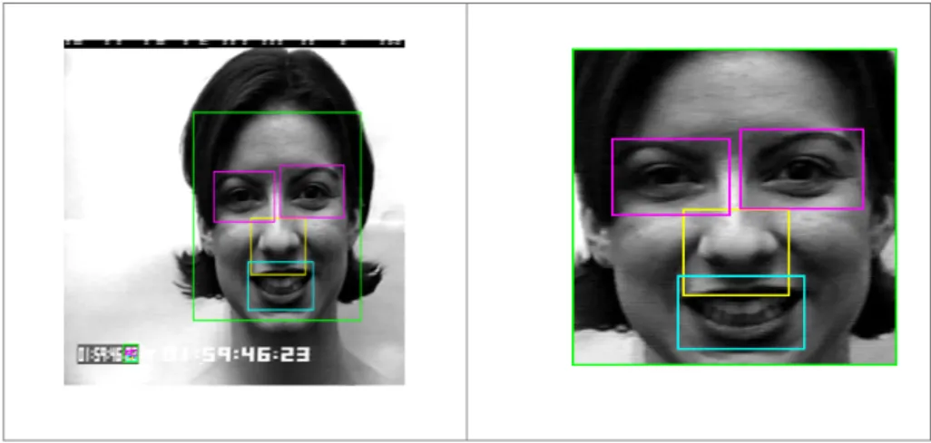
In CK dataset, the background is large with all the face images. First we apply the Viola-Jones algorithm to find the faces. For eyes, nose and mouth detection we applied cascaded object detector with region set on already detected frontal faces [Figure 4]. This cascade object detector with proper region set can identify the eyes, nose and mouth. Actually it uses Viola-Jones Algorithm as an underlying system. This object uses a cascade of classifiers to efficiently process image regions for the presence of a target object. Each stage in the cascade applies increasingly more complex binary classifiers, which allows the algorithm to rapidly reject regions that do not contain the target. If the desired object is not found at any stage in the cascade, the detector immediately rejects the region and processing is terminated.

9.2. Contrast Adjustment

The CK dataset varies greatly in image brightness. First we use Contrast Adjustment to enhance the image from very light images. Due to some reason when we apply the Histogram Equalization for very light images, the images distort. On the other side when apply Contrast Adjustment for very dark images, the images distort. As far of our knowledge, we are the first to separate the technical difference between Contrast Adjustment and Histogram Equalization. Contrast Adjustment works good for very light images as well as Histogram Equalization works good for very dark images from CK facial expression dataset.

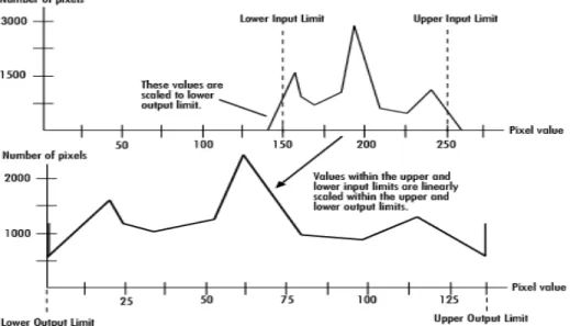
When an image lacks sharp difference between black and white, it means the image lacks contrast. For image Contrast Adjustment, first we set an upper and lower limit of pixel value. Then we linearly scale the pixel values of facial expression images between these preset upper and lower values. But which pixel values are above or below this range, we saturated those to the upper or lower limit value, respectively. Figure 5. depicts the process of Contrast Adjustment.

Figure 5. Contrast Adjustment Procedure

9.3. Histogram Equalization

As discussed in the previous subsection, to improve the contrast of the very dark images we apply Histogram equalization. We specify the histogram which is the output from the Contrast Adjustment process. By transforming the values of the dark images intensity it matches the specified histogram. The peaks of the histogram are widened and the valleys are compressed. So that the output is equalizes histogram.

9.4. Cropping

9.5. Training and Testing Data

We used here 100 subjects 1200 images and four face parts of the images. For every case (whole face, eyes, nose and mouth) we used 60% of the images for training and 40% for testing. We make separate face spaces for six different facial expressions. Then after ICA decomposition on the test images Euclidian distance is used for recognizing the closely match. When we applied ICA on whole faces, it happens that the system finds similar faces rather than similar expression when the same or similar person’s face is in the both the train and test folder. For this reason part based analysis, WAPA, OEPA and also LS-ICA performs better than whole face ICA decomposition.

10.

R

A

10.1. FastICA

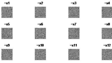
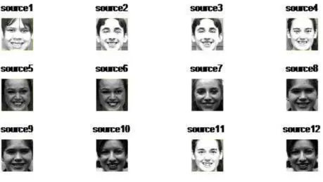
We performed differentiation on the vector of images as a preprocessing step. Figure 6. shows the filtered mixed signals after differentiation. Different source images are depicted in Figure 7. Independent components of the images are shown in Figure 8. Figure 9. Shows global 3D matrix of Performance Index. As described before Performance Index is a well known formula for measuring the separation performance which can be defined as

= =

− −

=

m

i n

j j i j j i

A A

n m A PI

1 1 ,

,

) 1 ] [ max

] [ ( )

1 (

1 )

( ………(10)

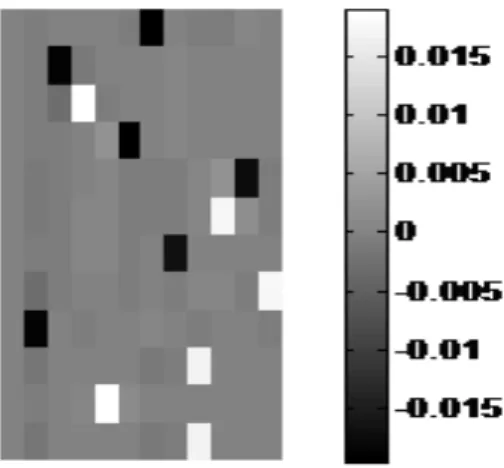
Where [A]_i,j is the (i,j) th-element of the matrix [A]. As because, the knowledge of the mixing matrix [A] is required, the smaller value of PI usually mentions the better performance evaluation for experimental settings. Finally Figure 10. Shows the estimated Inverse matrix.

Figure 7. Source images

Figure 8. Independent Components

Figure 10. Estimated Matrix Inverse (W)

10.2. FastICA with different Kernels

We implemented FastICA with three kernels: Hyper Tangent, Gaussian and Cubic kernels. Table 1. is a comparison among first ten independent component extraction time. This table clearly shows the Gaussian kernel needs the less time compared to other kernels of FastICA. So for the next step we choose the FastICA algorithm with Gaussian kernel.

Table 1. Time comparison among different kernels of FastICA algorithm. Algorith m Extracted Component Trial Iteratio n Elapsed Time Performance Index Fast ICA using Hyper tangent (tanh()y) Compone nt1 Compone nt2 Compone nt3 Compone nt4 Compone nt5 Compone nt6 Compone nt7 Compone nt8 Compone nt9 Compone 1 1 1 1 1 1 1 1 1 1 11 11 94 18 25 13 13 12 22 16

nt10 Fast ICA using Gauss (y*exp (-y^2/2)) Compone nt1 Compone nt2 Compone nt3 Compone nt4 Compone nt5 Compone nt6 Compone nt7 Compone nt8 Compone nt9 Compone nt10 1 1 1 1 1 1 1 1 1 1 11 11 15 16 58 32 25 13 41 12

45.11 s 0.1835

Fast ICA using Cubic (y^3) Compone nt1 Compone nt2 Compone nt3 Compone nt4 Compone nt5 Compone nt6 Compone nt7 Compone nt8 Compone nt9 Compone nt10 1 1 1 1 1 1 1 1 1 1 217 236 40 20 16 19 11 19 21 12

397.56 s 0.1329

10.3. Influence of Different Parts

both eyes and mouth are needed whereas only mouth is enough to achieve the highest accuracy of surprise expression. The other results are shown below.

Table 2: Effects of facial parts for expression recognition. LE=Left Eye, RE=Right Eye, N=Nose, M=Mouth, OEPA=Optimal Expression-specific Parts Accumulation

Facial Parts

Surpris e

Anger Sad Happy Fear Disgust

LE 82% 65% 66% 70% 40% 55%

RE 82% 65% 66% 70% 40% 55%

LE+RE 82% 65% 66% 70% 40% 55%

N 15% 15% 50% 15% 30% 55%

M 98% 50% 55% 90% 80% 50%

LE+RE+ N

60% 55% 50% 75% 56% 85%

LE+RE+ M

98% 80% 70% 100% 96% 80%

N+M 69% 50% 50% 60% 50% 70%

LE+RE+ N+M

85% 90% 86% 85% 85% 78%

WAPA-FastICA

92% 88% 82% 88% 90% 82%

OEPA-FastICA

98% (M)

90% (LE+RE+ N+M)

86% (LE+RE+N +M)

100% (LE+RE +M)

96% (LE+RE +M)

85% (LE+RE +N)

10.4. LS-ICA

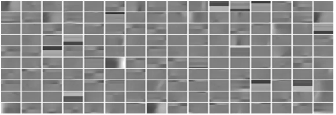
As described before the Locally Salient ICA (LS-ICA) has the ability to identify locally distorted parts more accurately. So we choose here LS-ICA to compare against FastICA methods even with the WAPA and OEPA based FastICA to understand which algorithm plays better role for specific applications of Facial Expression Recognition. Figure 11. shows a set of LS-ICA components after performing the LS-ICA decomposition over the images of facial expression.

11.

C

M

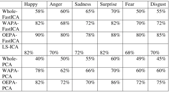
The following table (Table 3) shows the comparison among Whole face based ICA, Weighted All Parts Accunulation based FastICA, Optimal Expression Specific Parts Accumulation based FastICA, and Locally Salient ICA. For some expressions the LS-ICA outperforms the conventional FastICA and our proposed WAPA-FastICA methods. This is because LS-ICA algorithm has the strength to identify the local distortion more accurately. But the OEPA based FASTICA outperforms LS-ICA methods as we are choosing here only that facial parts which has the influence for specific facial expressions rather than choosing all the four face parts. Here we also compare these proposed methods with our proposed methods of previous published work [27]. In [27] we investigated PCA (Principal Component Analysis) on whole faces and also on different facial parts. To apply on different facial parts we propose two methods namely WAPA-PCA and OEPA-WAPA-PCA. In the following table and graph we will also show the comparison with these PCA methods. As we discussed in section 3, PCA works on second order derivatives and ICA on higher order derivatives and prominent features of facial expression images lie on high dimensional space. So overall recognition rate of ICA is better than PCA. Here our experiment also depicts the same evaluation.

Table 3. Comparison among proposed algorithms. (W-FastICA:Whole face ICA, WAPA:Weighted All Parts Accunulation, OEPA: Optimal Expression Specific Parts Accumulation, LS-ICA: Locally Salient

ICA.)

Happy Anger Sadness Surprise Fear Disgust

Whole-FastICA

58% 60% 65% 70% 50% 55%

WAPA-FastICA

82% 68% 72% 82% 70% 72%

OEPA-FastICA

90% 80% 78% 88% 80% 85%

LS-ICA 82%

70%

72%

82%

68%

70%

Whole-PCA

40% 50% 55% 60% 49% 45%

WAPA-PCA

78% 62% 66% 70% 60% 60%

OEPA-PCA

12.

In this work, our main focus is on Independent Component Analysis (ICA). Research shows that ICA has significant success on face image analysis. Among several architectures we mainly used here FastICA and LS-ICA. We apply FastICA with Gaussian kernel on whole faces and different facial parts like, eyes, mouth and nose. When we apply ICA on whole faces, the system finds similar faces rather than similar expression when the same or similar person’s face is in both train and test folder. For this reason, part based analysis, WAPA, OEPA and also LS-ICA performs better than the whole face ICA decomposition. Our experiment shows OEPA-FastICA outperforms W-FastICA, WAPA-FastICA and LS-ICA. Here we also compare these proposed methods with our proposed methods of previous published work [27]. In [27] we investigated PCA (Principal Component Analysis) on whole faces and also on different facial parts. To apply on different facial parts we propose two methods namely WAPA-PCA and OEPA-PCA. As PCA works on second order derivatives and ICA on higher order derivatives and prominent features of facial expression images lie on high dimensional space. So overall recognition rate of ICA is better than PCA and our experiment depicts the same evaluation.

A

R

[1] A. Hyvarinen, (1999) “Survey of Independent Component Analysis”, Neural Computing Surveys, 2:94-128.

[2] A.Hyvarinen & E.Oja, (2000) “Independent component analysis: Algorithms and application”, Neural Networks, 13(4-5):411- 430.

[3] A. Hyvarinen & E. Oja, (1997) “A fast fixed-point algorithm for independent component analysis”, Neural Computation, 9(7): 1483- 1492.

[4] A. Hyvarinen, R.Cristescu, & E.Oja, (1999) “A fast algorithm for estimating overcomplete ICA bases for image windows”, Proc.Int.Joint Conf. on Neural Networks, Pages 894-899,Washington, D.C. [5] T. Sergios, Pattern Recognition Book.

[6] Barlow H.B., (1989) “Unsupervised Learning”, Neural Computation, Vol. 1,pp. 295-311.

[7] S.B. Marian, J.R. Movellan & T. J. Sejnowski, (2002) “Face recognition by ICA”, IEEE Transactions on Neural Networks.

[8] S. B. Marian, R. M. Javier, & J. S. Terrence, (2002) “Face Recognition by Independent Component Analysis”, IEEE transaction Neural Networks, 13(6), 1450-1464.

[9] H. B. Barlow, (1989) “Unsupervised learning,” Neural Computing, vol. 1, pp. 295–311.

[10] J. J. Atick & A. N. Redlich, (1992) “What does the retina know about natural scenes?,” Neural Comput., vol. 4, pp. 196–210.

[11] G. Donato, M. S. Bartlett, J. C. Hagar, P. Ekman, & T. J. Sejnowski, (1999) “Classifying Facial Actions,” IEEE Transaction on Pattern Analysis and Machine Intelligence, vol. 21, no. 10, pp. 974-989.

[12] P. Ekman & W. V. Priesen, (1978) “Facial Action Coding System: A technique for the Measurement of Facial Movement,” Consulting Psychologists Press, Palo Alto, CA. Contributed Paper Manuscript received September 28, 2009 0098 3063/09/$20.00 © 2009 IEEE

[13] I. Buciu, C. Kotropoulos, & I. Pitas, (2003) “ICA and Gabor Representation for Facial Expression Recognition,” in Proceedings of the IEEE, pp. 855-858.

[14] F. Chen & K. Kotani, (2008) “Facial Expression Recognition by Supervised Independent Component Analysis Using MAP Estimation,” IEICE Transactions on Information and Systems, vol. E91-D, no. 2, pp. 341- 350.

[15] A. Hyvarinen, J. Karhunen, & E. Oja, (2001) “Independent Component Analysis,” John Wiley & Sons.

[16] Y. Karklin & M.S Lewicki, (2003) “Learning higher-order structures in natural images,” Network: Computation in Neural Systems, vol. 14, pp. 483-499.

[17] M. S. Bartlett, G. Donato, J. R. Movellan, J. C. Hager, P. Ekman, & T. J. Sejnowski, (1999) “Face Image Analysis for Expression Measurement and Detection of Deceit,” in Proceedings of the Sixth Joint Symposium on Neural Computation, pp. 8-15.

[18] C. Chao-Fa & F. Y. Shin, (2006) “Recognizing Facial Action Units Using Independent Component Analysis and Support Vector Machine,” Pattern Recognition, vol. 39, pp. 1795-1798.

[19] A. J. Calder, A. W. Young, & J. Keane, (2000) “Configural information in facial expression perception,” Journal of Experimental Psychology: Human Perception and Performance, vol. 26, no. 2, pp. 527-551.

[20] M. J. Lyons, S. Akamatsu, M. Kamachi, & J. Gyoba, (1998) “Coding facial expressions with Gabor wavelets,” in Proceedings of the Third IEEE International Conference on Automatic Face and Gesture Recognition, pp.200-205.

[21] M. S. Bartlett, J. R. Movellan, & T. J. Sejnowski, (2002) “Face Recognition by Independent Component Analysis,” IEEE Transaction on Neural Networks, vol. 13, no. 6, pp. 1450-1464.

[22] C. Liu, (2004) “Enhanced independent component analysis and its application to content based face image retrieval,” IEEE Transactions on Systems, Man, and Cybernetics-Part B: Cybernetics, vol. 34, no. 2, pp. 1117- 1127.

[24] A. B. Humayra, P. M. W. David, L. Richard & L. W. Trent, (2011) “Comparison of Region Based and Weighted Principal Component Analysis and Locally Salient ICA in Terms of Facial Expression Recognition”, 81-89. International Conference on Software Engineering, Artificial Intelligence, Networking and Parallel/Distributed Computing (SNPD), Springer, Sydney, Australia.

[25] A. B. Humayra and P. M. W. David, (2013) “Facial expression recognition based on Weighted All Parts Accumulation and Optimal Expression-specific Parts Accumulation”, The InternationalConference on Digital Image Computing: Techniques and Applications (DICTA) Hobart, Tasmania, Australia, page 229-235.

Authors Short Biography

1.Humayra Binte Ali is currently pursuing PhD in CSEM School of Flinders University, South Australia.She graduated form the dept of Computer science and Engineering, Dhaka University, Bangladesh, in 2007 with a first class honours. She was involved in research project of MAGICIAN, Multiple Autonomous Ground-robotic International Challenge by Intelligent Adelaide Navigators(2009-2010), in Flinders University. She also worked as a research assistant in Deakin University, Melbourne with the project of “Early Heart Rate Detection with Machine

Learning”. Her research interests are in pattern recognition, machine learning, computer vision, image analysis, cognitive neuroscience and facial

expression recognition.

2. Professor David M W Powers

Beijing Municipal Lab for Multimedia & Intelligent Software Beijing University of Technology

Beijing, China

KIT Centre, School of Comp.Sci., Eng. & Maths Flinders University