Proc. Estonian Acad. Sci. Geol., 2006, 55, 1, 3–23
Radiative characteristics of ice-covered fresh-
and brackish-water bodies
Helgi Arst
a, Ants Erm
b, Matti Leppäranta
c, and Anu Reinart
da
Estonian Marine Institute, University of Tartu, Mäealuse 10A, 12618 Tallinn, Estonia; helgi.arst@sea.ee
b
Marine Systems Institute, Tallinn University of Technology, Akadeemia tee 21B, 12618 Tallinn, Estonia; ants@phys.sea.ee
c
Division of Geophysics, University of Helsinki, P.O. Box 64, Fi-0014 Finland; matti.lepparanta@helsinki.fi
d
Tartu Observatory, Tartu county, Tõravere, Estonia; anu.reinart@ebc.uu.ee
Received 28 August 2005, in revised form 28 November 2005
Abstract. The structure and optics of ice and snow overlying bodies of water were studied in the years 2000–2003. The data were collected in the northern temperate region (nine Estonian and Finnish lakes and one brackish water site, Santala Bay, in the Gulf of Finland). In the present paper we describe the results concerning the radiative characteristics of the system “snow + ice cover on the water”: albedo, attenuation of light, and planar and scalar irradiances through the ice. The basic data consist of irradiance measurements above and below ice cover for the PAR band of the solar spectrum (400–700 nm). Albedo varied across wide limits (0.20–0.70 for ice, 0.63–0.94 for snow), depending on the optical and physical properties of ice/snow and weather conditions. The vertically averaged light attenuation coefficient of the ice layer in the brackish waters of Santala Bay was higher than that in the lakes. The ratio of irradiance beneath the ice to incident irradiance increased 2.5–20 times after removing the snow, depending on the albedo and the thickness of ice and snow as well as on their optical properties. In the upper layer of water beneath the ice the ratio of planar to scalar quantum irradiances increased with depth (according to our earlier results obtained in summer this ratio decreased with increasing depth).
Key words: ice optics, albedo, under-ice irradiance, euphotic zone.
INTRODUCTION
Oceanographic Tables 1975; Grenfell & Maykut 1977; Warren & Clarke 1990; Carroll & Fitch 1981; Warren 1982; Arrigo et al. 1991; Carlson et al. 1992; Allison et al. 1993; Grenfell et al. 1994; Kaup 1995; Rasmus 2003). However, the investigations of the system “snow + ice cover on the water” cannot be considered as complete without the results obtained in sub-polar and temperate regions. Snow and ice prevail in North European countries for about 5–7 months of the year and constitute an important research field for environmental sciences (ecology, geography, geophysics, and engineering). Note that in the Arctic and Antarctic snow and ice are mostly very clean. In few cases when the albedo for apparently clean snow occurred lower than usually, it was assumed that there was a grey absorber such as soot in the snow (Warren 1982; Grenfell et al. 1994). In sub-polar regions ice and snow are often formed on the water bodies with a notable concentration of optically active substances and contaminated also by atmospheric fallout. Consequently, the properties of snow/ice cover can notably differ from those in the Arctic and Antarctic.
Snow and ice are products of cold weather and precipitation, and therefore vary widely between the time of precipitation in autumn to spring as well as from year to year, in their thickness and properties (Michel & Ramseier 1971; Mullen & Warren 1988; Haendel et al. 1995; Perovich 1998; Granberg 1998; Leppäranta et al. 2003).An important part of the investigations is the optics of ice and snow – albedo, transparency, concentrations of optically active substances (OAS) – and under-ice light field. There are many publications concerning snow and ice hydro-logy, ice cover dynamics, and ice engineering, but the percentage of the optical studies is rather small. However, the data on the optical properties and radiative transfer in the system “snow/ice cover + water” are necessary for understanding the thermodynamics of covered lakes and seas, including the role of the ice-albedo-feedback mechanism. These data are also important for remote sensing models and for investigating the photosynthesis in early spring and late autumn.It has been shown that the ice cover affects phytoplankton photosynthesis in water (Fritsen & Priscu 1999). The optical properties of the ice cover on lakes and bays have been studied by Chekhin (1987), Mullen & Warren (1988), Maffione (1998), Semovski et al. (2000), Leppäranta et al. (2003), Erm et al. (2003), Ehn (2003), and Ishikawa et al. (2003).
A comprehensive study (in situ measurements, modelling, and comparison with the data of other authors in the region of 300–2600 nm) on the optical properties of snow has been conducted by Warren (1982). In Mullen & Warren (1988) a radiative transfer model was developed to illustrate the processes involved in determining the spectral albedo and transmission of lake ice (for the same region of the spectrum). The main objective of their investigation was to examine the link between ice microstructure (especially air bubbles in the ice) and the radiative properties.
were collected during many field trips in 2000–2003. The study sites were Estonian and Finnish lakes and one brackish-water area, Santala Bay, in the Gulf of Finland. The data consist of the concentrations of OAS in ice and under-ice water, the spectra of the beam attenuation coefficient for filtered and unfiltered water (for ice they are determined from meltwater), and the values of quantum irradiance above and below ice cover. Additionally, in some cases the vertical and crystal structures of the ice sheet (different types of sublayers) were investigated by photos in normal and polarized light. Part of the results obtained are published in Leppäranta et al. (2003), Erm & Reinart (2003), and Erm et al. (2003), where the analysis of the ice structure (including the formation of sublayers in ice cover), the amount of OAS, and some data on the under-ice light field is performed. Some of these data were also used in Arst & Sipelgas (2004), where the possibilities of describing the spatial variation and properties of the ice cover in water bodies by simultaneous in situ and satellite measurements are given. In the present study attention is focused on radiative characteristics of the system “snow + ice cover on the water”: albedo, attenuation of light, and planar and scalar irradiances under the ice. In addition to the data acquired in 2000–2001 used in earlier studies, it includes also the results obtained in winters 2002 and 2003.
MATERIALS AND METHODS
The planar and scalar irradiances at some depth z in the water can be defined in the following way (Dera 1992; Arst 2003):
2 2
d d
0 0
( ) d ( , , ) cos sin d ,
E z L z
π π
ϕ ϑ ϕ ϑ ϑ ϑ
=
∫
∫
(1)2
0
0 0
( ) d ( , , )sin d ,
E z L z
π π
ϕ ϑ ϕ ϑ ϑ
=
∫ ∫
(2)where E zd( ) is downwelling irradiance on a horizontal plane at depth z in the water and E z0( ) is scalar irradiance, Ld and L are radiances from the directions determined by azimuth angle ϕ and zenith angle ϑ. When Ed and E0 are the spectral values, then irradiance for the PAR region of the spectrum we obtain as integral over wavelength :λ
700
PAR 400
( )d
E =
∫
E λ λ (3)700
PAR
0 400
( ) d ,
q E
hc
λ
λ λ
=
∫
(4)where h=6.6255 10× −34 J s is Planck’s constant and c0 =2.9979 10× 8 m s–1 is the velocity of light in vacuum. As is generally known, qPAR is the suitable sum of light quanta necessary for photosynthesis.
The basic data of our study consist of irradiance measurements above and under ice cover, integrated over the PAR band (400–700 nm). Two quantum sensors (LI-192 SA and LI-193 SA, available from LI-COR, Inc. USA) were used, providing irradiance in units of µmol s–1 m–2. The former measures the downwelling planar irradiance, the latter measures the scalar irradiance. The data were collected in winters 2000–2003 in nine Estonian and Finnish lakes and in one brackish-water site, Santala Bay, in the Gulf of Finland (Table 1). However, the radiative properties of the snow/ice cover and under-ice water cannot be described in detail relying only on the numerical values of the irradiances. The under-ice light field is formed under the simultaneous influence of many factors: the values of incident irradiance (dependent on solar altitude and weather conditions), the presence of snow on the ice cover, thicknesses and optical properties of snow and ice, optical properties of under-ice water. As already mentioned, all results presented in this paper are obtained for the PAR region of the spectrum (400– 700 nm), but the index “PAR” was omitted for brevity.
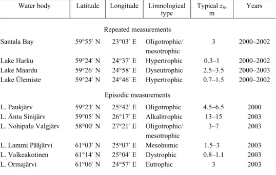
Table 1. Water bodies studied in winters 2000–2003 (typical values of the Secchi depth, zS, in the
ice-free period are also shown)
Water body Latitude Longitude Limnological type
Typical zS,
m
Years
Repeated measurements
Santala Bay 59°55′ N 23°03′ E Oligotrophic/ mesotrophic
3 2000–2002
Lake Harku 59°24′ N 24°37′ E Hypertrophic 0.3–1 2000–2002 Lake Maardu 59°26′ N 24°58′ E Dyseutrophic 2.5–3.5 2000–2003 Lake Ülemiste 59°24′ N 24°46′ E Hypertrophic 0.7–1.5 2000–2002
Episodic measurements
L. Paukjärv 59°23′ N 25°42′ E Oligotrophic 4.5–6.5 2000 L. Äntu Sinijärv 59°05′ N 26°17′ E Alkalitrophic 13–15 2003 L. Nohipalu Valgjärv 58°00′ N 27°21′ E Oligotrophic/
mesotrophic
3–7 2003
In our analysis of the contribution of these factors and for comparison of the radiative properties of different water bodies we decided to use the following characteristics produced from the irradiance data:
1. albedo of the ice (or snow) surface ( ),A
2. diffuse attenuation coefficient of light in under-ice water (Kd,w),
3. vertically averaged attenuation coefficient of light in the ice cover (Kd,i), 4. the ratio of incident irradiance to the value of irradiance just under the snow/ice
cover ( ),T and the respective ratio ( )Ta that is calculated after eliminating the irradiance which returns from the ice surface back to the atmosphere,
5. the ratio of plane irradiance to scalar irradiance in under-ice water (qd q0). Albedo was calculated as a ratio of upwelling irradiance to downwelling irradiance
u( 0) d( 0),
A=q z= q z= (5)
where the subscripts d and u are for downwelling and upwelling irradiance, respectively.
One of the parameters widely used in the optics of water bodies is the irradiance attenuation coefficient Kd (mostly called the “diffuse attenuation coefficient”). As is known (e.g. Dera 1992),
d d
d
d ( ) 1
( ) .
( ) d
q z K z
q z z
= − (6)
Note that this definition does not depend on angular distribution of radiance on which basis the irradiance is determined. Solution of this equation gives us
(7)
In studies of ice/snow optics (Warren 1982) in parallel the term “extinction coefficient” is used (its definition is analogous to Eq. (6)). This characteristic is usually reported in units of geometric depth, but it is possible to use also the units of liquid equivalent depth (Warren 1982). We preferred the geometric units (m–1), because in our study also the values of Kd for under-ice water are presented.
In general, Kd depends on depth, but when in the water layer from z1 to z2 it does not, we get:
d 2 d,w 1 2
2 1 d 1
( ) 1
( , ) ln .
( )
q z K z z
z z q z
= −
The index w means that we are investigating a water layer. When the layer is optically heterogeneous, then Kd,w( ,z z1 2) is the vertically averaged coefficient. Thus, when we have no data about the change of irradiance inside a layer of a medium, we can determine the vertically averaged Kd by measuring qd on the upper and lower surface of the layer. For the surface layer q zd( )1 = −(1 A q) (inc), where (inc)q is the incident irradiance.
In the ice layer the attenuation coefficient is vertically not variable since it contains sublayers with different optical properties. However, the attenuation of light in the ice cover can be approximately characterized, analogously to Eq. (8), using the vertically averaged attenuation coefficient of light:
d i d,i i
i
( ) 1
( ) ln ,
(1 ) (inc)
q D K D
D A q
= −
−
(9)
where Di is the thickness of the ice cover and (inc)q is the incident onto the upper ice surface solar irradiance. When Di is measured in metres, then Kd,i will be in m–1. The values of Kd,i calculated by Eq. (9) cannot describe the variation of optical properties inside the ice layer, but they do allow us to compare the light attenuation properties of ice covers in different lakes.
The diffuse attenuation coefficient Kd,w is an apparent optical property, depending not only on the optical properties of the medium, but also on illumination conditions (cloudiness, angular and spectral structures of incident irradiance). Incident irradiance is diffuse only when the sky is totally overcast. In other cases the radiance in the direction of the Sun considerably exceeds its values in any other direction. Under the water surface (without ice) the peak caused by direct solar radiation is clearly seen in upper layers, but (due to multiple scattering of light) it disappears gradually with increasing depth. Thus, as depth increases, the radiation becomes more diffuse, reaching at a certain depth an “asymptotic regime” (Ivanov 1975; Dera 1992; Kirk 1996). The change in the angular structure of light with depth depends on the type of the water: in eutrophic and hyper-trophic lakes it is rapid, in clear-water lakes it is slower. As far as under-ice water is concerned, the role of incident irradiance is played by the light that already penetrated the snow and/or ice layers, and its spectral and angular distributions are different in comparison with the light falling onto the upper surface of the snow/ice layer. In the ice layer a marked scattering of light is going on, due to the reflecting and scattering properties of ice crystals as well as air bubbles. A reliable assumption seems to be that the light that has penetrated through ice cover is already in some “diffuse regime”, i.e. the maximum in the direction of the Sun is not seen (except in case of thin and transparent ice). Thus, the angular distribution of radiation just below ice cover is more or less comparable with that in a deeper layer of ice-free water.
of the snow layer (i.e. inside the two-layer system) needs to be known. How-ever, we can estimate the transparency of this system calculating the ratios
T = qd(D)
&
qd(inc) and Ta = qd(D)&
(1–A)qd(inc), where D is the thickness of the ice or ice + snow layer. Denoting the thickness of the snow layer as Ds, we get D=Di+Ds. The ratio T shows how much incident irradiance remains at the lowest surface of the snow/ice layer, while for the ratio Ta we took into accountthat upwelling irradiance on the ice surface is Aqd(inc) and, therefore Ta
represents the transparency of the ice/snow layer after eliminating the irradiance which returns to the atmosphere. Consequently, Ta = T
&
(1–A) (both parameters are calculated using the same values of qd, Di, and Ds).For an entire water body or for an extensive water layer, the vertically averaged value of Kd,w is usually determined by performing regression analysis on a semilog plot of irradiance vs. depth (Dera 1992; Reinart & Herlevi 1999; Arst et al. 2000). Note that the exponential law (Eq. (7)) is totally correct only for spectral irradiance, but is widely used also for estimating the values of the attenuation coefficient, averaged over the PAR region. The respective errors for ice-free water bodies are estimated in Arst et al. (2000).
A suitable parameter describing the angular structure of the under-ice light field is the ratio of planar to scalar irradiances qd q0. This ratio can be mathematically expressed in the following way (see Eqs (1) and (2)):
2 2
d
d 0 0
2 2 2
0
d u
0 0 0
2
d ( , )sin cos d
.
d ( , )sin d d ( , )sin d
L q
q
L L
π π
π
π π π
π
ϕ ϕ ϑ ϑ ϑ ϑ
ϕ ϕ ϑ ϑ ϑ ϕ ϕ ϑ ϑ ϑ
=
+
∫
∫
∫
∫
∫
∫
(10)
Here q0 is given as the sum of two parts, downwelling and upwelling:
d d
0 0,d 0,u
q q
q =q +q . (11)
under-ice waters, because the light having just penetrated the under-ice layer is considerably more diffuse than that below the surface of ice-free water.
For the irradiance measurements under ice cover, a special device was constructed (Fig. 1). First, consoles (2) are placed alongside the telescopic probe. Then, the device is lowered into the water through a 30 cm hole in the ice and fastened on the tripod (3). Finally, the consoles are positioned horizontally using cords (4). By changing the length of the probe and the inclination of the legs of the tripod, the desired measurement depth can be selected. The system allows the measurements of irradiance at about 1 m from the ice hole in the horizontal direction down to a depth of 1.5–2 m.
The sensors used in this device were LI-192 SA (planar irradiance) and LI-193 SA (scalar irradiance). Planar (or downward vector) irradiance is the irradiance coming from an upper hemisphere onto a plane surface while scalar irradiance is the irradiance onto a sphere (Jerlov 1968). Both sensors measure in the PAR region (400–700 nm) and have been separately calibrated for quantum irradiance. In the air the quantum irradiance of 4.6 µmol s–1 m–2 corresponds to a radiative energy of 1 W m–2 but in the water this relationship depends on water properties (Reinart & Arst 1998). In 2000 we measured only incident and underwater irradiances, however since 2001 we have used four sensors: two under-ice (LI-192 SA and LI-193 SA) and two LI-192 SA sensors in air (at the height of 1 m from the ice surface), simultaneously measuring up- and downwelling irradiance. This enabled us to measure simultaneously also the albedo values for the PAR region. The instruments were first lowered into the water and then brought back to the surface, irradiances were recorded in both cases. To examine the horizontal patchiness in the optical properties of ice cover, the procedure was repeated changing the directions of LI-192 SA and LI-193 SA by 180°. When-ever snow covered the ice, it was removed and the measurements were repeated. A datalogger LI-1400 (LI-COR, Inc. USA) was used to record results.
Our main investigation sites were located between 59°24′ and 59°55′ N, but a few measurements were performed also for three Estonian and three Finnish lakes between 58° and 61°06′ N. Some information on the water bodies studied is presented in Table 1. The measurements were made mostly between 10:00 and 15:00 hours, with solar altitudes varying from 15° in January to 30° in March. Note that there were some cases where we were unable to measure every parameter (due to strong wind, snowfall or technical problems).
RESULTS AND DISCUSSION Albedo
As is known, some incident (onto the ice layer) irradiance returns to the atmosphere, some is absorbed (after multiple scattering) in the ice layer, and some penetrates through the layer. According to Eq. (5), albedo is determined as the ratio of upwelling irradiance to downwelling irradiance. Upwelling irradiance just above the the snow/ice layer consists of radiation reflected from the surface and radiation backscattered from different depths of the snow/ice layer. The amount of radiation reflected/backscattered from snow/ice crystals as well as that lost due to absorption/scattering processes inside the layer depend on the structure and optical properties of the layers. The values of downwelling irradiance just below the ice layer depend on three parameters: (1) incident irradiance, (2) albedo, and (3) light attenuation coefficient inside the layer.
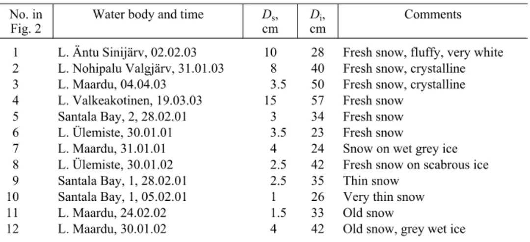
Fig. 2. Change in the albedo in the PAR region of the spectrum after removing snow from ice cover. The numbers on the x-axis are explained in Table 2.
A(snow) and A(snow removed), mainly caused by variations of optical properties of ice and snow (Fig. 2; Table 2). In most cases A(snow removed) exceeds 0.5, which is systematically higher than A(ice). This is explained not only by the greyness of some types of ice and/or the melting ice (smaller scattering coefficients), but also by the fact that, especially in case of scabrous ice, we cannot totally remove all the snow: some snow invariably remains on the ice and increases its albedo. Without the snow the values of A(ice) vary between 0.20 and 0.58, the higher figure occurring when hoarfrost is on the ice. Our limited database (especially for the vertical and crystal structure of ice) did not allow us to carry out a reliable investigation on the relationships between albedo and ice micro-structure.
Table 2. Comments to Fig. 2 (thicknesses of the snow cover (Ds) and ice layer (Di) are also shown)
No. in Fig. 2
Water body and time Ds,
cm Di,
cm
Comments
1 L. Äntu Sinijärv, 02.02.03 10 28 Fresh snow, fluffy, very white 2 L. Nohipalu Valgjärv, 31.01.03 8 40 Fresh snow, crystalline 3 L. Maardu, 04.04.03 3.5 50 Fresh snow, crystalline 4 L. Valkeakotinen, 19.03.03 15 57 Fresh snow
5 Santala Bay, 2, 28.02.01 3 34 Fresh snow 6 L. Ülemiste, 30.01.01 3.5 23 Fresh snow
7 L. Maardu, 31.01.01 4 24 Snow on wet grey ice 8 L. Ülemiste, 30.01.02 2.5 42 Fresh snow on scabrous ice 9 Santala Bay, 1, 28.02.01 2.5 35 Thin snow
10 Santala Bay, 1, 05.02.01 1 26 Very thin snow 11 L. Maardu, 24.02.02 1.5 33 Old snow
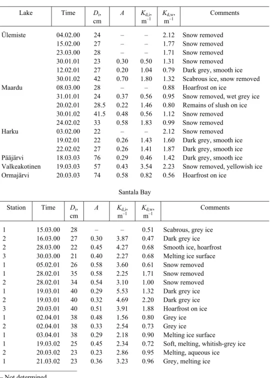
Table 3. Values of the albedo (A), vertically averaged attenuation coefficient of light for ice (Kd,i),
and diffuse attenuation coefficient for under-ice water (Kd,w), all for the PAR region of the spectrum.
Only the cases without snow are presented. Di is the thickness of the ice layer
Lakes
Lake Time Di,
cm
A Kd,i,
m–1 Kd,w,
m–1
Comments
Ülemiste 04.02.00 24 – – 2.12 Snow removed
15.02.00 27 – – 1.77 Snow removed
23.03.00 28 – – 1.71 Snow removed
30.01.01 23 0.30 0.50 1.31 Snow removed
12.02.01 27 0.20 1.04 0.79 Dark grey, smooth ice 30.01.02 42 0.70 1.80 1.32 Scabrous ice, snow removed Maardu 08.03.00 28 – – 0.88 Hoarfrost on ice 31.01.01 24 0.37 0.56 0.95 Snow removed, wet grey ice
20.02.01 28.5 0.22 1.46 0.80 Remains of slush on ice 30.01.02 41.5 0.48 0.56 1.12 Snow removed
24.02.02 33 0.58 1.83 0.99 Snow removed
Harku 03.02.00 22 – – 2.12 Snow removed 19.02.01 22 0.26 1.43 1.60 Dark grey, smooth ice 22.02.02 27 0.26 1.41 1.87 Dark grey, smooth ice Pääjärvi 18.03.03 76 0.29 0.46 1.42 Dark grey, smooth ice Valkeakotinen 19.03.03 57 0.43 3.54 2.23 Snow removed, yellowish ice Ormajärvi 20.03.03 74 0.58 0.82 0.56 Hoarfrost on ice
Santala Bay
Station Time Di,
cm
A Kd,i,
m–1
Kd,w,
m–1
Comments
1 15.03.00 28 – – 0.51 Scabrous, grey ice 2 16.03.00 27 0.30 3.87 0.47 Dark grey ice 2 28.03.00 22 0.45 4.27 0.68 Smooth ice, hoarfrost 3 30.03.00 21 0.40 2.27 0.68 Melting ice surface 1 05.02.01 26 0.58 3.60 0.61 Snow removed 1 28.02.01 35 0.58 2.25 1.71 Snow removed 2 28.02.01 34 0.54 3.10 1.00 Snow removed 1 19.03.01 40 0.29 5.53 1.32 Dark grey ice 2 19.03.01 40 0.32 4.69 2.20 Dark grey ice 3 20.03.01 40 0.51 3.91 1.88 Hoarfrost on ice 1 02.04.01 38 0.48 1.56 0.80 Grey ice 2 02.04.01 38 0.33 2.54 0.73 Grey ice 1 03.04.01 38 0.29 2.18 0.90 Melting ice surface
1 19.03.02 25 0.45 2.34 0.72 Soft, melting, whitish-grey ice 2 20.03.02 23 0.23 2.86 0.95 Melting, aqueous ice
1 21.03.02 23 0.36 3.23 0.96 Grey, melting ice _______________________
Data published in Oceanographic Tables (1975) place the albedo of fresh and dry snow in the limits of 0.80–0.95 (these values decrease as snow ages), and the albedo of melting snow in the limits of 0.30–0.40. For ice albedo only the data for Arctic seas are presented, varying between 0.4 and 0.7. However, obviously these values are not restricted to the PAR region, but cover the whole solar spectrum. Kaup (1995), measuring integral albedo in six lakes in East Antarctica, obtained 0.74–0.90 for snow and 0.13–0.59 for ice. According to his results taken in the Antarctic winter, lake ice was mostly without snow and rather transparent (A = 0.17–0.40), but at the time of the melting period the ice was whitish, with an albedo of 0.44–0.52. Perovich (1998) gives the typical values of A for an ice-covered sea: 0.87, 0.77, 0.70, and 0.30, respectively for snow, melting snow, ice, and melting ice. However, for the PAR band he gives about 0.9 for cold snow, 0.75 for cold bare ice, and 0.65 for melting snow. According to Ishikawa et al. (2003), the total albedo measured in lake waters at the Tvarminne biological station (Finland) was about 0.8 for snow, 0.30–0.35 for thick ice, and 0.1–0.2 for thin (Di < 10 cm)
ice. Data can be found in the literature about the spectral distribution of snow albedo (Warren 1982; Grenfell et al. 1994; Rasmus 2003) and lake ice albedo (Mullen & Warren 1988) in the region of 300–2500 nm. Several peaks (mainly in near infrared) were observed, but between 400 and 700 nm there was only very slight decrease in
A towards longer wavelengths. For instance, in case of diffuse illumination A(snow) decreased from 0.982 at 400 nm to 0.956 at 708 nm (Grenfell et al. 1994). Model calculations for lake ice with a thickness of 0.025 m (Mullen & Warren 1988) showed that, due to different conditions brought about by air bubbles, the spectral values of A in the PAR region can vary from 0.12 to 0.54, but only very slight decrease (about 3%) in A with increasing wavelength was observed. Rasmus et al. (2002) measured spectral albedo in Santala Bay. According to their data fresh snow albedos were between 0.8 and 0.9 and almost constant in the PAR band. In Rasmus (2003) the data on the Antarctic snow are presented: in the region of 400–700 nm albedo was 0.90–0.96 and decreased slowly towards greater wavelengths. Of course, there can be cases (old snow, melting ice, etc.), where the spectral change of A in the PAR region is larger. However, it seems that spectral albedo in the PAR region only slightly differs from the integral albedo for this region.
Diffuse attenuation coefficient
of Kd,w(PAR) (also shown in Table 3) were obtained by applying a semilog plot of qd(PAR) vs. depth in the water layer down to 1.5–2 m (Dera 1992; Reinart & Herlevi 1999; Arst et al. 2000). Comparison of the values of Kd,i and Kd,w shows that for lakes Kd,i can be higher or lower than respective Kd,w, but in Santala Bay we always obtained Kd,i>Kd,w. The ratios Kd,i Kd,w were, respectively, 0.3–1.8 and 1.3–8. Note that according to Chekhin (1987), in lake waters Kd,w
always exceeds Kd,i, but our data (including rather turbid lakes) support this conclusion only for 50% of observations.
Ratios T = qd(D)/qd(inc) and Ta = qd(D)/(1 – A)qd(inc)
The values of irradiance on the lower surface of ice cover depend on qd(inc), albedo, and the absorption/scattering properties of ice cover. As already mentioned, the values of T do not allow us to separate the influence of albedo from the influence of other ice properties. Of course, the value of albedo and light attenuation properties of ice are not independent. However, albedo is formed mainly due to reflecting properties of ice; the attenuation of light in the ice layer is a direct consequence of the absorbing and scattering properties of ice. For instance, in four cases of Table 3 albedo has the same value of 0.58, corresponding to the irradiance attenuation coefficients (Kd,i) 0.62, 1.83, 2.25, and 3.60 m–1. Some examples describing the values of T and Ta (with and without snow cover) are presented in Table 4. We can see marked differences between the cases “snow + ice” and “snow removed”. Note that, by using our whole database coupled with the results obtained, the removal of snow caused T to increase by about 2.5–20 times. The “snow + ice” cases in Table 4 give values of Ta that exceed the respective values of T by 2.6–14 times, while for cases “snow removed” this range is from 1.4 to 2.8. The influence of snow can also be estimated by values of Tsnow Tice and Ta,snow Ta,ice. These ratios varied, respectively, from 0.05 to 0.22 and from 0.18 to 0.46. Thus, as concluded in our earlier publications (Reinart 2000; Leppäranta et al. 2003; Arst & Sipelgas 2004), snow is the main factor reducing irradiance during its penetration through snow + ice cover.
Table 4. Some examples of the values of T = qd(D)/qd(inc) and Ta = qd(D)/(1 – A)qd(inc), (in %)
with and without snow cover on the ice. The thicknesses of ice and ice + snow layers (Di and
D = Di + Ds, respectively) are also shown
Snow + ice cover Snow removed Water body Time
D, cm T Ta Di, cm T Ta
L. Maardu 01.02.01 25.5 8.4 22 24 52 82 L. Ülemiste 30.01.01 26.5 4.4 23 23 58 83 Santala Bay, 1 06.02.01 31 6 21 25 27 64
L. Maardu 30.01.02 37 1.6 8 33 23 44
Underwater quantum irradiance and the ratio qd/q0
During the measurements the sensors LI-192 SA and LI-193 SA were first lowered and then brought back to the surface. An example of the vertical profiles of qd and q0 (below the system “snow + ice” and after removing the snow, both averaged using “down” and “up” series) is presented in Fig. 3. As expected,
d 0
q <q and both markedly increase after removing the snow from ice. We can also see that scalar irradiance decreases with increasing depth more rapidly than planar irradiance. This means that the diffuse attenuation coefficient for scalar irradiance in under-ice water exceeds that for planar irradiance. Qualitatively the same results we obtained relying on the other irradiance profiles in our dataset. These data are of interest, because in the surface layer of ice-free water bodies the opposite result was obtained (Kirk 1996; Reinart & Herlevi 1999; Reinart 2000).
The influence of patchiness of ice cover on the irradiance results was clearly detected on 28 March 2000 in Santala Bay and on 20 February 2001 in Lake Maardu (dark smooth ice with whitish patches of hoarfrost). The values of qd
and q0 under the whitish patch were about 11–26% smaller than under the smooth ice without hoarfrost. However, our device allowed us to measure qd and q0
only with a distance of 2 m from each other. To make some other ice holes and to repeat the measurements was technically complicated. Thorough investigation of horizontal variation of under-ice irradiance in conditions of ice patchiness requires repeated measurements in a number of ice holes located at some distance from each other.
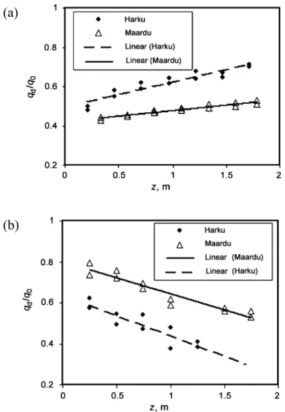
It is of interest to study the vertical change in qd q0 in the under-ice water and compute the slope ( )s of the respective regression line. There are estimations on the values of qd q0 in ice-free waters (Kirk 1996; Reinart 2000). These values
Fig. 3. Vertical profiles of qd and q0 (for the PAR region of the spectrum) below ice/snow cover and
after removing the snow (Di = 27 cm, Ds = 1.5 cm) in Lake Ülemiste on 15 February 2000.
depend markedly on the ratio b a, where b and a are, respectively, scattering and absorption coefficients of the solar beam. Kirk (1996) performed Monte Carlo calculations for vertically incident monochromatic light and showed that the ratio qd q0 changes from 0.9 to 0.43 when b a increases from 2 to 30. Reinart (2000) obtained the results for the PAR region in lakewater. The minimum value of qd q0 was 0.34 (hypertrophic Lake Tuusulanjärvi in Finland) and maximum 0.9 (oligotrophic Lake Paukjärv in Estonia). According to these estimations, the values of qd q0 exceeding 0.95 and below 0.3 have to be considered as unreliable.
A typical vertical distribution of qd q0 that we obtained for an ice-free oligo-trophic lake is shown in Fig. 4. We can see that in the surface layer the ratio
d 0
q q decreases with increasing depth. However, at the depths where angular structure of underwater light reaches the asymptotic state (Kirk 1996), qd q0
practically does not change any more (in the case presented in Fig. 4 it is around 5 m). In 1999–2003 we conducted numerous summer measurements in Estonian and Finnish lakes (altogether more than 80 profiles of qd q0). According to these results, the slope ( )s of the regression line qd q0 vs. depth in the surface layer varied from 0 to –0.2 m–1. Naturally, s is different for the layers at different depths; for example, in Lake Paukjärv (Fig. 4) the value of s in the layer of 0–2 m is –0.068 m–1, but in the “asymptotic” layer (z>4.5 m) it is –0.0017 m–1. Similarly, in the other lakes (Koorküla Valgjärv, Nohipalu Valgjärv), where the asymptotic part of the qd q0 profile was identified, the respective slopes in this layer were extremely small. Note that in some lakes (mostly yellow-coloured), where the scattering of light is relatively small, qd q0 can be almost constant from the surface downward and s is close to zero for the whole water column. It is difficult to ascertain the “asymptotic part” of the qd q0 profile in turbid lakes, because with growing depth the irradiance decreases very quickly and measurement errors are marked. Thus, according to these results, the values of the slope of
d 0
q q vs. depth in the ice-free surface layer are negative or close to zero.
Fig. 4. Depth-dependence of the ratio qd/q0 measured on 9 May 2000 (ice-free water) in Lake
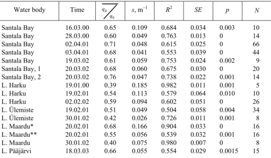
Relying on our winter data, we calculated the depth-averaged values of qd q0
and the statistical characteristics of its vertical distribution in the layer under the ice surface (down to about 2 m). Some examples (snow-free cases, where the determination coefficient R2 exceeded 0.5) are presented in Table 5. Note that the low values of R2 were typical of profiles, whose slopes are very small. How-ever, many of these cases were characterized by a small scattering of points along the (almost horizontal) regression line. This shows that on the basis of only R2
we cannot decide whether our data for “low-slope cases” are reliable or not. As is known, the regression is considered statistically significant (i.e. the results are reliable) when significance p<0.05. For most of our data the values of p were close to zero and SE was below 0.07. As already mentioned, removing the snow caused the decrease in qd q0 of about 10–30%.
As we can see in Table 5, averaged qd q0 varied between 0.39 and 0.76, being rather instable in lakes and more stable (0.60–0.76) in Santala Bay. How-ever, the most interesting result of these computations is that under ice/snow cover we got either close to zero or positive values of the slope (in the latter case qd q0 increases with depth). According to our whole database, we obtained values of s between –0.01 and 0.2 m–1 (of 35 profiles only 3 were negative slope values). This was to be expected because q0 decreases more quickly than qd in under-ice conditions (see Fig. 3). Some examples of the “winter” and “summer”
Table 5. The values of qd/q0 under ice cover (averaged over depth in the layer with a thickness of
about 2 m) and the statistical characteristics of its vertical distribution (only cases without snow and when R2> 0.5 are presented): s is the slope of the regression line of qd/q0 vs. depth, R
2
is the determination coefficient, SE is standard error, p is significance, and N is the number of points in each case of regression
Water body Time d 0
q
q s, m
–1 R2
SE p N
Santala Bay 16.03.00 0.65 0.109 0.684 0.034 0.003 10 Santala Bay 28.03.00 0.60 0.049 0.763 0.013 0 14 Santala Bay 02.04.01 0.71 0.048 0.615 0.025 0 66 Santala Bay 03.04.01 0.68 0.041 0.553 0.039 0 44 Santala Bay 19.03.02 0.61 0.059 0.753 0.024 0.002 9 Santala Bay, 1 20.03.02 0.68 0.060 0.675 0.030 0 20 Santala Bay, 2 20.03.02 0.76 0.047 0.738 0.022 0.001 14 L. Harku 19.01.00 0.39 0.185 0.982 0.011 0.001 5 L. Harku 19.02.01 0.54 0.113 0.579 0.064 0.010 10 L. Harku 02.02.02 0.59 0.094 0.602 0.051 0 26 L. Ülemiste 19.02.01 0.51 0.049 0.504 0.058 0.004 34 L. Ülemiste 30.01.02 0.42 0.026 0.726 0.011 0.001 8 L. Maardu* 20.02.01 0.68 0.166 0.904 0.033 0 16 L. Maardu** 20.02.01 0.55 0.056 0.539 0.032 0.001 16 L. Maardu 30.01.02 0.40 0.075 0.980 0.007 0 8 L. Pääjärvi 18.03.03 0.66 0.055 0.554 0.029 0.0015 15 ______________________
* Under dark patch, ** under whitish patch.
qd
slopes are presented in Fig. 5. Note that for extremely turbid Lake Harku we got the maximum absolute values of s (both in winter and summer).
To explain these results, we note that, first, the influence of snow/ice cover causes radiation to be highly diffuse just under the ice. Under ice-free conditions (on clear days) the asymptotic state of the angular structure of light is usually reached at deeper layers, but in ice-covered waters the profiles of qd q0 are already “asymptotic” beginning from the lower surface of ice. It is also important that in the ice-free water the radiation falling on the surface of the “asymptotic
Fig. 5. Depth-dependence of qd/q0 in the surface layer of two lakes and the corresponding regression
lines: (a) winter measurements, for Lake Harku s = 0.127 m–1, for Lake Maardu s = 0.057 m–1; (b) summer measurements, for Lake Harku s = –0.199 m–1, for Lake Maardu s = –0.155 m–1.
(a)
layer” originates from the same medium (water), but the radiation below the ice comes from a different medium (ice). The scattering properties of ice are much different from those of water. For a detailed analysis of the vertical profiles of qd
and q0 under ice cover the measurements of the angular structure of light at different depths are needed.
Euphotic zone in under-ice water
The concept of the euphotic zone is widely used in marine biology and marine optics, being generally applied to the water layer where photosynthesis takes place (Chekhin 1987; Morel & Berthon 1989; Adamenko et al. 1991; Dera 1992; Kirk 1996; Reinart et al. 2000). The thickness of the layer that is suitable for photosynthesis depends on the absolute values of surface irradiance and the diffuse attenuation coefficient of water, as well as on water temperature, the amount of nutrients, and the properties of phytoplankton. Most often (e.g. Morel & Berthon 1989; Koenings & Edmundson 1991; Kirk 1996; Wild-Allen et al. 2002) the euphotic zone is treated as the water layer at whose lower boundary the photo-synthetically active radiation falls to 1% of that just below the water surface (depth denoted by (1%)).z To estimate (1%)z for under-ice water, we cannot apply the formulae used for ice-free water (Kirk 1996; Reinart et al. 2000; Arst 2003), but we can discover the depth, where qd is equal to 1% from (inc).q Thus, the values of (1%)z in the under-ice water were estimated on the basis of measured profiles of qd, and, if necessary, these profiles were extrapolated using exponential law.
As expected, (1%)z depends on the thickness and optical properties of ice cover and, of course, the water properties. For lakes (1%)z varied from 0.53 to 4.7 m, in Santala Bay from 1.1 to 5.4 m (results for the cases without snow). The minimum “lake” values of (1%)z were observed in Lake Valkeakotinen in March 2003 (dystrophic lake, D=57cm). When the ice was covered with snow, then
(1%)
z was 0–1.3 m (data only for lakes). We also investigated the correlation between the variables. Note that for Santala Bay (all cases without snow) there was no strong relationship between (1%)z and the thickness of the ice layer. The parameter (1%)z practically does not correlate with (inc),q the correlation coefficients being below 0.3. Using our “lakes + Santala” database, we obtained a relationship for (1%)z vs. ,T where the correlation coefficient R=0.77.
CONCLUSIONS
2. The values of the vertically averaged diffuse attenuation coefficient of the ice layer (Kd,i) in Santala Bay were always higher than those in the lakes. One of the main reasons is probably the algal growth in the brine pockets of brackish sea ice, but Kd,i can notably also depend on the microstructure of each sub-layer of the ice. Comparison of Kd,i with Kd,w showed that the value of Kd,i
for freshwater lakes can be higher or lower than respective Kd,w, but in brackish water of Santala Bay we always obtained Kd,i>Kd,w. The ratios Kd,i Kd,w
for lakes and Santala Bay were, respectively, 0.3–1.8 and 1.3–8.
3. Similarly to our earlier results, the present study showed that snow is the main factor involved in the reduction of irradiance during its penetration through snow + ice cover. The values of the ratio T =q D qd( ) d(inc) increased after removing the snow 2.5–20 times, depending on the albedos and thicknesses of ice and snow as well as on their optical properties.
4. In under-ice water the scalar irradiance decreases with increasing depth more rapidly than planar irradiance. As a result, the ratio qd q0 increases with depth, i.e. the respective slope ( )s of the regression line is close to zero or positive (the maximum value was 0.2). Our earlier results, which were obtained in summer, showed that the values of s are close to zero or negative in ice-free periods (i.e. qd q0 is almost constant or decreases with increasing depth), depending on optical properties of water.
5. The euphotic zone (the water layer where photosynthesis takes place) is usually treated as the layer at whose lower boundary the photosynthetically active radiation falls to 1% of that just below the water surface (depth denoted by (1%)).z For lakes (1%)z varied from 0.53 to 4.7 m, in Santala Bay from 1.1 to 5.4 m (data for snow-free cases). When the ice was covered with snow, then (1%)z was 0–1.3 m.
ACKNOWLEDGEMENTS
The authors are indebted to the Estonian Science Foundation (grant No. 3613) and Väisala Foundation (Finland) for financial support to this investigation. We are also grateful to Liis Sipelgas for assistance in field-work.
REFERENCES
Adamenko, V. N., Kondratyev, K. Ya., Pozdnyakov, D. V. & Chekhin, L. P. 1991. Radiative Regime and Optical Properties of Lakes. Gidrometeoizdat, Leningrad (in Russian).
Allison, I., Brandt, R. E. & Warren, S. G. 1993. East Antarctic sea ice: albedo, thickness distribution and snow cover. J. Geophys. Res., 98, 12417–12429.
Arrigo, K. R., Sullivan, C. W. & Kremer, J. N. 1991. A biological model of Antarctic sea ice. J. Geophys. Res., 96, 10581–10592.
Arst, H. 2003. Optical Properties and Remote Sensing of Multicomponental Water Bodies. Springer, Praxis-Publishing; Chichester, U.K.
Arst, H., Reinart, A., Erm, A. & Hussainov, M. 2000. Influence of depth-dependence of the PAR diffuse attenuation coefficient on the computation of downward irradiance in different water bodies. Geophysica, 36, 129–139.
Bannister, T. T. 1992. Model of the mean cosine of underwater radiance and estimation of under-water scalar irradiance. Limnol. Oceanogr., 37, 773–780.
Carlson, R. W., Arakelian, T. & Smythe, W. D. 1992. Spectral reflectance of Antarctic snow: “Ground truth” and spacecraft measurements. Antarct. J. US, 27, 296–298.
Carroll, J. J. & Fitch, B. W. 1981. Dependence of snow albedos on solar elevation and cloudiness at the south pole. J. Geophys. Res., 86, 5271–5276.
Chekhin, L. P. 1987. Light Regime in the Water Bodies. Karelia Section of the Academy of Sciences USSR, Petrozavodsk (in Russian).
Dera, J. 1992. Marine Physics. PWN, Warszawa, ELSEVIER, Amsterdam.
Ehn, J. 2003. Optical properties of sea ice and seawater in Santala Bay. Rep. Ser. Geophys., 46, 101–106.
Erm, A. & Reinart, A. 2003. Optical properties of the system “ice cover + water” in different types of water bodies. In Proceedings of the Fourth Workshop on Baltic Sea Ice Climate, Norrköping, Sweden (Omstedt, A. & Axell, L., eds), Oceanografi SMHI, 72, 1–10.
Erm, A., Reinart, A., Arst, H., Sipelgas, L. & Leppäranta, M. 2003. Optical properties of lake and sea ice. Rep. Ser. Geophys., 46, 93–100.
Fritsen, C. H. & Priscu, J. C. 1999. Seasonal change in the optical properties of the permanent ice cover on Lake Bonney, Antarctica: consequences for lake productivity and phytoplankton dynamics. Limnol. Oceanogr., 44, 447–454.
Granberg, H. B. 1998. Snow cover on sea ice. In Physics of Ice-Covered Seas (Leppäranta, M., ed.), pp. 605–651. Helsinki University Printing House.
Grenfell, T. C. & Maykut, G. A. 1977. The optical properties of ice and snow in the Arctic Basin. J. Glaciol., 18, 445–463.
Grenfell, T. C., Warren, S. G. & Mullen, P. C. 1994. Reflection of solar radiation by the Antarctic snow surface at ultraviolet, visible and near-infrared wavelengths. J. Geophys. Res., 99, 18,669–18,684.
Haendel, D., Kaup, E., Loopmann, A. & Wand, U. 1995. Physical and hydrochemical properties of water bodies. In The Schirmacher Oasis, Queen Maud Land, East Antarctica (Bormann, P. & Fritsche, D., eds.), pp. 279–311. Justus Perthes Verlag, Gotha (Petermanns Geographische Mitteilungen, 289).
Hanson, K. 1960. Radiation measurements on the Antarctic snowfield: a preliminary report. J. Geophys. Res., 65, 935–946.
Ishikawa, N., Takizawa, A., Kawamura, T., Shirasawa, K. & Leppäranta, M. 2003. Changes of the radiation property with sea ice growth in Saroma Lagoon and the Baltic Sea. Rep. Ser. Geophys., 46, 147–160.
Ivanov, A. P. 1975. Physical Grounds of Hydrooptics. Nauka i tekhnika, Minsk (in Russian). Jerlov, N. G. 1968. Optical Oceanography. Elsevier Oceanographic Series, Elsevier, Amsterdam. Kaup, E. 1995. Solar radiation in water bodies. In The Schirmacher Oasis, Queen Maud Land, East
Antarctica and Its Surroundings (Bormann, P. & Fritsche, D., eds), pp. 286–290. Perthes, Gotha.
Kirk, J. T. O. 1996. Light and Photosynthesis in Aquatic Ecosystems. Cambridge University Press. Koenings, J. P. & Edmundson, J. A. 1991. Secchi disk and photometer estimates of light regimes in
Alaskan lakes: effects of yellow colour and turbidity. Limnol. Oceanogr., 36, 91–105. Leppäranta, M., Reinart, A., Erm, A., Arst, H., Hussainov, M. & Sipelgas, L. 2003. Investigation of
ice and water properties and under-ice light field in fresh and brackish water bodies. Nord. Hydrol., 34, 245–266.
Maffione, R. A. 1998. Theoretical developments on the optical properties of highly turbid water and sea ice.Limnol. Oceanogr., 43, 29–33.
Morel, A. & Berthon, J.-F. 1989. Surface pigments, algal biomass, and potential production of the euphotic layer: relationships reinvestigated in view of remote-sensing applications. Limnol. Oceanogr., 34, 1545–1562.
Mullen, P. C. & Warren, S. G. 1988. Theory of the optical properties of lake ice. J. Geophys. Res.,
93, D7, 8403–8414.
Oceanographic Tables. 1975. Gidrometeoizdat, Leningrad (in Russian).
Perovich, D. K. 1998. The optical properties of the sea ice. In Physics of Ice-Covered Seas (Leppäranta, M., ed.), pp. 195–230. Helsinki University Printing House.
Rasmus, K. 2003. The albedo of Antarctic snow. Rep. Ser. Geophys., 46, 73–78.
Rasmus, K., Ehn, J., Granskog, M., Kärkäs, E., Leppäranta, M., Lindfors, A., Pelkonen, A., Rasmus, S. & Reinart, A. 2002. Optical measurements of sea ice in the Gulf of Finland. Nord. Hydrol.,
33, 207–226.
Reinart, A. 2000. Underwater light field characteristics in different types of Estonian and Finnish lakes. Diss. Geophys. Univ. Tartuensis, 11.
Reinart, A. & Arst, H. 1998. Relation between underwater irradiance and quantum irradiance in dependence on water transparency at different depths in water bodies. J. Geophys. Res.,
103, C4, 7749–7752.
Reinart, A. & Herlevi, A. 1999. Diffuse attenuation coefficient in some Estonian and Finnish lakes. Proc. Estonian Acad. Sci. Biol. Ecol., 48, 267–283.
Reinart, A., Arst, H., Nõges, P. & Nõges, T. 2000. Comparison of euphotic layer criteria in lakes. Geophysica, 36, 141–159.
Semovski, S. V., Mogilev, N. Yu. & Sherstyankin, P. P. 2000. Lake Baikal ice: analysis of AVHRR imagery and simulation of under-ice phytoplankton bloom. J. Mar. Syst., 27, 117–130. Warren, S. G. 1982. Optical properties of snow. Rev. Geophys. Space Phys., 20, 67–89.
Warren, S. G. & Clarke, A. D. 1990. Soot in the atmosphere and snow surface of Antarctica. J. Geophys. Res., 95, 1811–1816.
Wild-Allen, K., Lane, A. & Tett, P. 2002. Phytoplankton, sediment and optical observations in Netherlands coastal waters in spring. J. Sea Res., 47, 303–315.