A technique for generating consistent ice sheet initial conditions for coupled ice-sheet/climate models

(1)

GMDD

6, 2491–2516, 2013

Ice sheet spin-up for coupled models

J. G. Fyke et al.

Title Page

Abstract Introduction

Conclusions References

Tables Figures

◭ ◮

Back Close

Full Screen / Esc

Printer-friendly Version Interactive Discussion

Discussion

P

a

per

|

Dis

cussion

P

a

per

|

Discussion

P

a

per

|

Discussio

n

P

a

per

|

Geosci. Model Dev. Discuss., 6, 2491–2516, 2013 www.geosci-model-dev-discuss.net/6/2491/2013/ doi:10.5194/gmdd-6-2491-2013

Geoscientiic Geoscientiic

Geoscientiic

Open Access

Geoscientiic Model Development Discussions

This discussion paper is/has been under review for the journal Geoscientific Model Development (GMD). Please refer to the corresponding final paper in GMD if available.

A technique for generating consistent ice

sheet initial conditions for coupled

ice-sheet/climate models

J. G. Fyke1, W. J. Sacks2, and W. H. Lipscomb1

1

Group T-3, Los Alamos National Laboratory, Los Alamos, New Mexico, USA

2

National Center for Atmospheric Research, Boulder, Colorado, USA

Received: 19 March 2013 – Accepted: 27 March 2013 – Published: 15 April 2013

Correspondence to: J. G. Fyke (fyke@lanl.gov)

(2)

GMDD

6, 2491–2516, 2013

J. G. Fyke et al.

Title Page

Tables Figures

◭ ◮

Back Close

Full Screen / Esc

Discussion

P

a

per

|

Dis

cussion

P

a

per

|

Discussion

P

a

per

|

Discussio

n

P

a

per

|

Abstract

A new technique for generating ice sheet preindustrial 1850 initial conditions for cou-pled ice-sheet/climate models is developed and demonstrated over the Greenland Ice Sheet using the Community Earth System Model (CESM). Paleoclimate end-member simulations and ice core data are used to derive continuous surface mass balance 5

fields which are used to force a long transient ice sheet model simulation. The proce-dure accounts for the evolution of climate through the last glacial period and converges to a simulated preindustrial 1850 ice sheet that is geometrically and thermodynamically consistent with the 1850 preindustrial simulated CESM state, yet contains a transient memory of past climate that compares well to observations and independent model 10

studies. This allows future coupled ice-sheet/climate projections of climate change that include ice sheets to integrate the effect of past climate conditions on the state of the Greenland Ice Sheet, while maintaining system-wide continuity between past and fu-ture climate simulations.

1 Introduction

15

Ice sheets play an important role in regulating critical aspects of the climate system such as sea level rise (Foster and Rohling, 2013), atmospheric circulation (Ridley et al., 2005) and ocean circulation (Weaver et al., 2003). Ice sheets can be considered cou-pled components of the climate system for several reasons. Ice sheet geometry is closely related to climate via the surface mass balance (SMB) and surface tempera-20

ture. SMB determines where ice accumulates or melts and thus helps set the ice sheet geometry. The surface temperature of the ice sheet is also set by the climate; this signal advects and di_ffuses into the ice sheet where it interacts with frictional and geothermal heat signals to set the internal ice temperature distribution. The internal temperature plays an important role in long-term ice dynamics by affecting ice rheology and limiting 25

(3)

GMDD

6, 2491–2516, 2013

J. G. Fyke et al.

Title Page

Tables Figures

◭ ◮

Back Close

Full Screen / Esc

Discussion

P

a

per

|

Dis

cussion

P

a

per

|

Discussion

P

a

per

|

Discussio

n

P

a

per

|

melting point (Cuffey and Patterson, 2010). Conversely, ice sheets influence regional-to-hemispheric circulation patterns, oceanic freshwater fluxes and regional tempera-tures.

Coupled ice-sheet/climate models are powerful tools for constraining the behavior of ice sheets because they capture important feedbacks between ice sheets and climate 5

and calculate the SMB using in-line energy balance calculations. Thus, an increasing number of fully coupled ice-sheet/climate models are in active development and have recently been used to perform a wide range of experiments (Vizca´ıno et al., 2010; Fyke et al., 2011; Lipscomb et al., 2013; Gregory et al., 2012). An important aspect of coupled ice-sheet/climate simulations is generation of consistent initial coupled climate 10

and ice sheet conditions. In coupled climate models, full system consistency between all components of the climate model is required before prognostic experiments can proceed. In traditional non-ice-sheet-enabled models consistency is gained via spin-up from some initial condition, often observations, and integrated forward with coupling between components enabled. Ice sheets excluded, the bottleneck to full climate sys-15

tem equilibration is typically the deep ocean which equilibrates on the order of∼103yr. Given the first-order stability of the late Holocene, equilibrium initial conditions for future climate change simulations are typically generated by spin-ups under constant prein-dustrial 1850 external forcing such that at year 1850 all the components of the climate are in equilibrium with each other and with the constant external forcing.

20

Inclusion of ice sheets in coupled models renders this traditional “equilibrium” spin-up approach problematic. Ice sheets reach quasi-equilibrium on the order of average deep ice residence and lithospheric relaxation timescales, ∼104−105yr. The present-day Greenland and Antarctic ice sheets (GIS/AIS) thus contain a thermal memory of past glacial periods that influences present-day and future ice sheet dynamics. In addition to 25

the thermal signature, Antarctica may still be responding directly to residual geometric imbalances from the last deglaciation (Huybrechts and LeMeur, 1999).

(4)

GMDD

6, 2491–2516, 2013

J. G. Fyke et al.

Title Page

Tables Figures

◭ ◮

Back Close

Full Screen / Esc

Discussion

P

a

per

|

Dis

cussion

P

a

per

|

Discussion

P

a

per

|

Discussio

n

P

a

per

|

models has been to use computationally inexpensive climate drivers to spin-up through at least one previous glacial-interglacial cycle prior to future projections. This generates ice sheet states with reasonable preindustrial 1850 internal temperature fields and a potential non-equilibrium dynamic drift. The climate forcing is typically obtained through the use of paleoclimate time series (often oxygen isotope records) as drivers of cali-5

brated, spatially-distributed, time-varying mass balance and temperature fields (e.g. Cuffey and Marshall, 2000; Applegate et al., 2012). These techniques have the ad-vantage of being computationally cheap. Also, users are relatively free to adjust the climate forcing such that the resulting calibrated ice sheet reasonably approximates present-day.

10

Unlike standalone ice sheet models, fully coupled ice-sheet/climate models cannot currently perform long synchronous spin-ups. The basic obstacle is computational ex-pense: full climate models (or even climate models of intermediate complexity) cannot typically run synchronously for 104to 105yr, which is the length of time required to in-still ice sheet components of the model with proper history-dependent internal temper-15

atures. Additionally, the complex interactions between components of a coupled model and the requirements of global mass and energy conservation in most global mod-els make it impossible to apply simple calibrations to any in-line SMB model. Existing attempts to circumvent these basic problems in coupled models that use an energy balance model for SMB display various shortcomings. For example:

20

– A computationally cheaper climate parameterization could be used to force an ice sheet model through one or more glacial periods (Vizca´ıno et al., 2010). At some point, the resulting ice sheet could be inserted into the climate model. However, this approach results in an artificial discontinuity in the ice dynamic response due to a step-function change in climate forcing that potentially affects future simula-25

tions.

(5)

GMDD

6, 2491–2516, 2013

J. G. Fyke et al.

Title Page

Tables Figures

◭ ◮

Back Close

Full Screen / Esc

Discussion

P

a

per

|

Dis

cussion

P

a

per

|

Discussion

P

a

per

|

Discussio

n

P

a

per

|

1850 temperature/precipitation conditions calculated using paleoclimate time series. However, an analogous approach to scaling inputs to the SMB model is not feasible for full energy balance-based SMB models. Also, if a PDD model is used during spin-up, a discontinuity will occur when the transition to the energy balance model occurs.

5

– Asynchronous coupling could be used to accelerate the ice sheet and orbital forc-ings, relative to the rest of the climate. However, abyssal ocean and ice sheet-related limits to asynchronicity (Calov et al., 2009) still necessitate an extremely long climate simulation of 10 kyr or more to cover the entirety of the last glacial cycle.

10

– The ice sheet/climate model could be spun up under constant preindustrial 1850 forcing. However, this neglects any effect of climate history on preindustrial 1850 ice sheet conditions.

These issues point to a need for alternate methods for generating spun-up ice sheets for use in coupled models, that have reasonable internal memories of past climate yet 15

are consistent with the simulated preindustrial 1850 climate. Here, we explore one such method with the Community Earth System Model (CESM).

A summary of this paper is as follows: in Sect. 2 we detail important aspects of the SMB model, the procedure for generating transient SMB forcing for the last glacial pe-riod and how this forcing drives an ice sheet model. In Sect. 3 we demonstrate the 20

ability of this method to simulate a preindustrial 1850 ice sheet state that is consis-tent with the simulated preindustrial 1850 and past climate model states. Section 4 describes potential future ice sheet and climate model developments that could im-prove the spun-up preindustrial 1850 ice sheet state. We also contrast spin-up of ice sheet models against inversion-based initialization methods in the context of coupled 25

(6)

GMDD

6, 2491–2516, 2013

J. G. Fyke et al.

Title Page

Tables Figures

◭ ◮

Back Close

Full Screen / Esc

Discussion

P

a

per

|

Dis

cussion

P

a

per

|

Discussion

P

a

per

|

Discussio

n

P

a

per

|

2 Methodology

The ice sheet spin-up technique described here can be briefly described as follows: a climate model is used to simulate Last Glacial Maximum (LGM), mid-Holocene Opti-mum (MHO) and preindustrial 1850 climate states, from which equilibrium 30-yr SMB climatology matrices at all (x,y,z) locations over Greenland are extracted. Composite 5

SMBs at times between these climate end-members are then calculated using weight-ing based on the NGRIP ice coreδO18record (Wolffet al., 2010).

2.1 End-member SMB generation

Previously, Brady et al. (2013) generated fully-coupled equilibrium climate states for the LGM and MHO using the Community Climate System Model 4. The same model 10

was also spun up under 1850 conditions (Landrum et al., 2012). Included in the output of each of these simulations were the necessary fields required to drive standalone Community Land Model (CLM) simulations. The final 30 yr of data from each of these simulations were used to drive three standalone CLM V4.0 (Oleson et al., 2010) “IG” simulations, which included calculations for generating in-line SMB values for multiple 15

elevation classes over the Greenland landmass. The final 30 yr of SMB for each CLM simulation were then downscaled (Lipscomb et al., 2013) and used as end-member forcings for a 122 kyr standalone 5 km resolution, shallow-ice-approximation Commu-nity Ice Sheet Model (CISM1) simulation. 30-yr SMB climatologies (as opposed to a simple mean SMB climatology) were used to ensure any non-zero effects on SMB due 20

to inter annual variability (Pritchard et al., 2008) were properly captured.

An advantage of the CLM SMB calculations is the use of sub-grid “virtual” elevation classes, where SMB calculations are carried out even if no ice exists at a given ele-vation at run-time (the area of these virtual land areas is set to zero during run-time, but SMB values are still saved to file). This feature allows for calculation of physically 25

(7)

GMDD

6, 2491–2516, 2013

J. G. Fyke et al.

Title Page

Tables Figures

◭ ◮

Back Close

Full Screen / Esc

Discussion

P

a

per

|

Dis

cussion

P

a

per

|

Discussion

P

a

per

|

Discussio

n

P

a

per

|

(x,y,z) space, it is always in contact with SMB values. This avoids complexities related to generating SMB lapse rates (Helsen et al., 2012) and allows climate model-derived SMB values to be used directly during the ice sheet model simulation.

2.2 Continuous paleo-SMB forcing generation

Standalone ice sheet spin-up procedures aimed at generating a reasonable preindus-5

trial 1850 GIS are typically initialized at the Last Interglacial (LIG) or earlier and run forward for full length of the last glacial cycle to ensure a proper imprint of past cli-mate on preindustrial 1850 ice sheet conditions. Given the basic lack of an appropriate CESM coupled LIG simulation, we assumed the MHO to be the best approximation for the LIG and copied this forcing for use as idealized initial end-member LIG SMB 10

forcing. The bias in ice sheet evolution resulting from MHO forcing in place of LIG forcing has little effect on the final preindustrial 1850 ice sheet state (which is the pri-mary target of the simulation) since the memory of this forcing is largely swept from the system during the∼50 kyr cold glacial period (Sect. 3). To recreate the transient climate signal seen over the GIS during the last glacial epoch, a technique from stan-15

dalone ice sheet model spin-ups was adopted and modified. First, representative LGM, MHO and preindustrial 1850δO18values were determined by averaging 600 yr of nor-malized NGRIP values bounding each time period (for the preindustrial 1850, NGRIP values corresponding to the interval 1250–1850 were used) from the NGRIP δO18 record (Wolffet al., 2010). A 600-yr average value was used to avoid aliasing of end 20

member NGRIP values due to high-frequency variability in the NGRIP record. The NGRIP time series was then thresholded slightly to account for the fact that time peri-ods represented by the climate model end member simulations did not fall exactly on maximum/minimum MHO/LGM NGRIP values. This avoided extrapolation of SMB val-ues beyond the cold/warm LGM/MHO cases, which would have potentially introduced 25

(8)

GMDD

6, 2491–2516, 2013

J. G. Fyke et al.

Title Page

Tables Figures

◭ ◮

Back Close

Full Screen / Esc

Discussion

P

a

per

|

Dis

cussion

P

a

per

|

Discussion

P

a

per

|

Discussio

n

P

a

per

|

SMB values of cold pre-LGM glacial interstadials to LGM values, despite suggestions from the isotopic record that these periods were potentially more extreme.

The thresholded NGRIP-derived time series was then used as an interpolation weighting function to calculate SMB for any time and location in Greenland between the LIG and preindustrial year 1850. Climate was assumed constant over 600-yr in-5

tervals. For each interval, a weight between bracketing end-members was determined via an average of the NGRIP values contained in the 600-yr period. A looped, 30 yr climatology was then constructed for this period by a linear combination of SMB values from the appropriate years of the bounding end-member climates:

←−

wt= δ

18

OEM₊₁−δ18OCC

δ18_O

EM₊₁−δ18OEM₋₁

(1) 10

−→

wt=1−←wt− (2)

SMB(x,y,z)yr_CC=1:30=[SMB(x,y,z)yr←−−=1:30

EM ←−

wt]+[SMB(x,y,z)yr−−→=1:30

EM −→

wt] (3)

←−−

EM and −EM represent bounding end member climates for a particular mid-run cli-−→ mate period CC. For example, for a period CC in midst of the last glacial period, 15

←−−

EM=LIG and−EM−→=LGM.

The resulting daisy-chain of looped climatologies provides the time-continuous forc-ing for the long standalone ice sheet simulation. A main advantage of the procedure is that it converges towards the simulated preindustrial 1850 climatological SMB forcing at year 1850. Thus, the ice sheet at 1850 will be in thermodynamic consistency with 20

both the simulated preindustrial 1850 climate, and pre-1850 climate evolution.

(9)

GMDD

6, 2491–2516, 2013

J. G. Fyke et al.

Title Page

Tables Figures

◭ ◮

Back Close

Full Screen / Esc

Discussion

P

a

per

|

Dis

cussion

P

a

per

|

Discussion

P

a

per

|

Discussio

n

P

a

per

|

presented in Lipscomb et al. (2013), some additional model changes have been im-plemented. The number of elevation columns was increased to 36, the maximum snow depth was increased to 5 m water equivalent and a sub-grid snow-rain partitioning rou-tine to segregate incoming precipitation based on downscaled surface temperature was included.

5

3 Results

A simulation was performed to evaluate the ability of the procedure to generate a prein-dustrial 1850 ice sheet state that was consistent with climate model forcing. In the fol-lowing discussion this simulation is termed the “transient” spin-up. To gauge the impact of the spin-up technique on the state of the ice sheet at 1850 a parallel simulation (the 10

“equilibrium” spin-up) was carried out in which a similarly-configured ice sheet model was forced with constant preindustrial 1850 conditions.

3.1 Evolution of surface forcing conditions

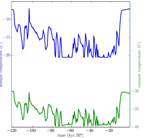
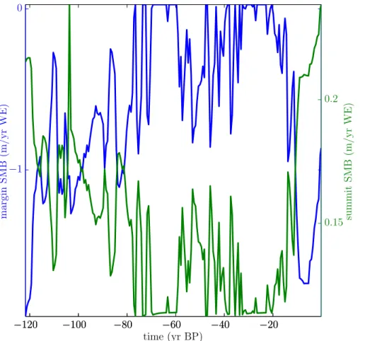
An important aspect of the procedure is its ability to generate physically reasonable transient forcing fields for the ice sheet model throughout the course of the simulation. 15

Figures 1 and 2 show the evolution of temperature and SMB in the surface layer of the ice sheet model at the observed summit and a western ablation zone location. A comparison of these two time series highlights important strengths of the spin-up tech-nique. Near-surface temperature trends on the margin are similar to interior trends. As expected, temperatures in both regions decrease during glacial periods. The tempera-20

(10)

GMDD

6, 2491–2516, 2013

J. G. Fyke et al.

Title Page

Tables Figures

◭ ◮

Back Close

Full Screen / Esc

Discussion

P

a

per

|

Dis

cussion

P

a

per

|

Discussion

P

a

per

|

Discussio

n

P

a

per

|

marginal location are always warmer than those in the interior, ranging from−7◦C to −21◦C.

Conversely, SMB trends in the interior are generally anti-correlated to trends on the margin. During a glacial state, summit SMB decreases from over 0.2 m yr−1 _{LWE to}

0.11 m yr−1

LWE, in excellent agreement with accumulation rates derived from the 5

GRIP ice core (Dahl-Jensen et al., 1993). On the other hand, margin SMB increases from−2 m yr−1LWE to 0.05 m yr−1. The opposite response of the two locations results from a lack of ablation in the interior and decreased atmospheric moisture transport in glacial climates. At the summit, since no ablation occurs at any time, the simu-lated decrease in precipitation during glacial periods causes a decrease in SMB. This 10

decrease is due to a combination of decreased moisture availability from increased sea ice cover, decreased marine boundary layer evaporative potential, and decreased moisture-carrying capacity of cold air. Reproduction of the interior SMB decrease in glacial climates is thus realistic and serves as a validation of the basic climate model physics. In contrast, marginal SMB increases strongly during glacial periods. This is 15

simply due to a reduction in ablation during glacial periods which overwhelms any rel-atively small decrease in accumulation.

3.2 Evolution of ice sheet temperature

The ice sheet model was initialized at 122 ka with a present-day geometry based on a modified version of Bamber et al. (2001) and an internal temperature profile that 20

trended linearly from a modeled preindustrial 1850 surface temperature to the location-specific pressure-dependent melting point, minus 2◦_{C. From this initial condition the}

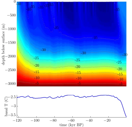
transient temperature and SMB forcings drove a thermal ice sheet response. Figure 3a plots the evolution of internal temperatures for the ice underlying the observed summit location. The first∼20 kyr of simulation are dominated by the slow spin-up of the ice 25

(11)

GMDD

6, 2491–2516, 2013

J. G. Fyke et al.

Title Page

Tables Figures

◭ ◮

Back Close

Full Screen / Esc

Discussion

P

a

per

|

Dis

cussion

P

a

per

|

Discussion

P

a

per

|

Discussio

n

P

a

per

|

characterized by the strong penetration of cold LGM ice into the interior of the ice sheet. The deglacial transition to the warm early-mid Holocene is well-captured in internal temperatures. The last∼10 kyr of the simulation are unique for the strong inversion in the upper temperature profile as cold glacial ice is buried under significantly warmer deglacial and Holocene ice; at its strongest, ice near the surface is up to 5◦

C warmer 5

than ice at mid-depths. This inversion decreases with time as the cold glacial signal advects margin-wards and the transition from the MHO to the preindustrial 1850 cools the upper ice.

The basal temperature shows a very damped response to surface temperatures changes. However, the extended cold signal of the LGM is sufficient to penetrate to 10

the bottom of the ice sheet in these simulations and is actively depressing the basal temperatures at 1850. This delayed present-day cooling response to LGM conditions is occurring at the same time that shallower regions of the central ice sheet display warming, highlighting the multiple response thermodynamic timescales inherent in the GIS.

15

3.3 Evolution of ice sheet geometry

The geometry of the ice sheet evolves freely in time as the simulation proceeds. The ice summit elevation and location migrates in response to the interior SMB. During glacial periods the strong decrease in precipitation in the interior is reflected by a 100– 200 m drop in the summit elevation and an eastward summit migration of∼75 km. At 20

the same time, margins of the ice sheet thicken due to decreased ablation. The net effect of these two processes is a decrease in ice volume during glacial periods since the decrease in volume in the interior outweighs the increase in marginal thickening. This trend towards increasing ice volume during warmer periods is potentially biased by the general overestimation of margin extent in the model: in many places around the 25

(12)

GMDD

6, 2491–2516, 2013

J. G. Fyke et al.

Title Page

Tables Figures

◭ ◮

Back Close

Full Screen / Esc

Discussion

P

a

per

|

Dis

cussion

P

a

per

|

Discussion

P

a

per

|

Discussio

n

P

a

per

|

and growth during glacial periods, allowing the influence of interior volume changes to dominate. This e_ffect is due to climate-derived SMB biases (Lipscomb et al., 2013) and as such we note that future improvements to the SMB fields generated by CESM could change the characteristics of the evolution of ice sheet volume during the spin-up procedure.

5

3.4 Comparison of transient spin-up to equilibrium spin-up at 1850

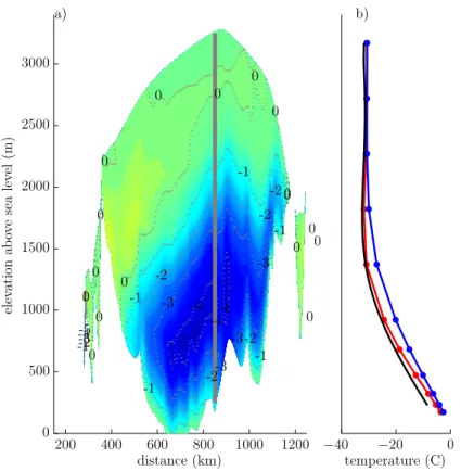
A comparison of the transient spin-up to the equilibrium spin-up at the end of the sim-ulation highlights the impact of integrating a realistic climate history into the ice sheet. Figure 4a plots the di_fference in internal temperatures at 1850, across the same cross-section that contains the summit column plotted previously. The difference in temper-10

atures is small (less than 1◦_{C) in the upper ice column, but increases to almost 5}◦_C

in the deep interior. Figure 4b plots the observed GRIP temperature profile (Green-land Ice-Core Project (GRIP) Members, 1993) against both the GRIP-site transient and equilibrium spin-up profiles at 1850. The transient spin-up does a significantly better job at matching the GRIP temperature profile. The agreement between the observed and 15

transient spin-up temperature profiles confirms the spin-up procedure’s first-order abil-ity to capture past ice history accurately despite being driven solely by climate model output. The temperature at the base of the GRIP core location is significantly warmer than observed in both models (though less so in the case of the transient spin-up): this is due to a too-high prescribed geothermal heat flux in this location in the model 20

and/or slight spatial biases within the ice sheet model (a∼40 km shift in the location of simulated temperature profile would provide a much better basal comparison).

Differences in basal temperatures between the equilibrium and transient spin-up sim-ulations are shown in Fig. 5. The transient spin-up displays colder basal temperatures in the interior, with temperatures up to 5◦

C colder along the major ice divides. The 25

(13)

GMDD

6, 2491–2516, 2013

J. G. Fyke et al.

Title Page

Tables Figures

◭ ◮

Back Close

Full Screen / Esc

Discussion

P

a

per

|

Dis

cussion

P

a

per

|

Discussion

P

a

per

|

Discussio

n

P

a

per

|

regions of the model which experience basal sliding, compared to the equilibrium spin-up case.

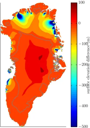
Differences in surface elevation between the two spin-ups are shown in Fig. 6. The transient spin-up displays large decreases in ice thickness (up to 500 m) in the northern ice sheet relative to the equilibrium spin-up. This di_fference arises from the extended 5

simulated warm period of the MHO during which ablation is notably higher around the ice sheet margin (Fig. 2), resulting in margin retreat relative to the equilibrium spin-up. The interior of the ice sheet is slightly higher than the equilibrium spin-up case, po-tentially due to the influence of increased precipitation during the MHO. Both of these effects move the 1850 preindustrial state closer to the observed ice sheet geometry 10

compared to the equilibrium spin-up simulation. Over the final 4200 yr of the simula-tion, the ice sheet is gaining ice volume at a modest rate of 9 km3yr−1

, in agreement with the estimate of 20 km3yr−1 _{made by Huybrechts (1994). The spatial pattern of}

surface elevation change dH/dt also agrees qualitatively with Huybrechts (1994), in that the recent mass gain is concentrated at the margins of the ice sheet, particularly 15

the southwest. These results suggest that it may be necessary to integrate not only LGM climate but also more recent Holocene climate trends into any ice sheet spin-up procedure in order to accurately capture the large-scale preindustrial 1850 GIS state.

4 Discussion

In Sects. 2 and 3 we described and demonstrated a technique for generating ice sheet 20

initial conditions for use in future simulations that are thermodynamically consistent with forcing from 1850 preindustrial and paleoclimate climate model simulations. The procedure involves generation of end-member SMB and surface temperature matri-ces from climate model simulations, followed by a standalone ice sheet model simula-tion through the last glacial period with forcing derived from interpolated end-member 25

(14)

GMDD

6, 2491–2516, 2013

J. G. Fyke et al.

Title Page

Tables Figures

◭ ◮

Back Close

Full Screen / Esc

Discussion

P

a

per

|

Dis

cussion

P

a

per

|

Discussion

P

a

per

|

Discussio

n

P

a

per

|

novelty of the present procedure is that it extends these techniques by utilizing energy-balanced SMB values generated by a climate model, specifically to generate an ice sheet state that is amenable for use in fully coupled ice-sheet/climate simulations.

A requirement for accurate spin-up of an ice sheet model is consistent SMB and temperature forcing fields. Temperature distribution in the interior of the ice sheet is 5

controlled is large part by ice advection which in turn is a strong function of accumu-lation rate (e.g. SMB). In turn, ice temperature controls internal deformation rates via the temperature dependence of ice rheology and also regulates where basal sliding can occur. The final spun-up ice sheet geometry is therefore a function of both past temperature and past SMB; this dual dependency is captured by the procedure de-10

scribed here. In contrast, spin-up processes that insert a scaled spun-up temperature profile from one ice sheet model into another prior to coupled ice-sheet/climate simu-lations risk non-physical dynamic transients, potentially out to the timescale of thermal equilibrium of the ice sheet,∼20 kyr.

Inverse procedures (e.g. Arthern and Gudmundsson, 2010) have been recently used 15

to calculate basal drag coefficient fields such that the difference between simulated and observed velocities is minimized. However, it is not clear that such methods are fea-sible alternatives to the approach described here, for fully-coupled ice-sheet/climate models. Since coupled models are in no way constrained by observations, an equi-librated coupled model representation of the preindustrial 1850 will invariably display 20

biases compared to observations (including biases in ice sheet state): this is the trade-offfor full system consistency. Conversely, an ice sheet state that is in force balance and reproduces observed velocities will display very small biases but will very likely be inconsistent with any model-derived climate. As a specific example, if an ice sheet ini-tialized by an observationally-constrained inverse method was inserted into the CESM 25

(15)

GMDD

6, 2491–2516, 2013

J. G. Fyke et al.

Title Page

Tables Figures

◭ ◮

Back Close

Full Screen / Esc

Discussion

P

a

per

|

Dis

cussion

P

a

per

|

Discussion

P

a

per

|

Discussio

n

P

a

per

|

drag coefficient field results in an ice sheet that best respects both observed velocities and modeled surface conditions (Price et al., 2011). However, additional issues could arise. For example, any SMB biases would not be removed but simply transferred to basal traction coefficient field biases of the ice sheet model. Also, any ice sheet model in a coupled model must be allowed to expand into ice-free regions. For example, cur-5

rent CESM climate forcing simulates perennial snow cover and thus in-situ ice sheet growth in several initially ice-free marginal GIS regions during the transient spin-up. It is not clear how inversion techniques could properly account for this climate-dependent growth of ice, the presence of which is necessary for simulated preindustrial 1850 cli-mate consistency and certainly for coupled simulations of colder clicli-mate periods such 10

as the LGM.

Several recent studies have utilized large ensembles of ice sheet simulations to opti-mize important ice sheet model parameters (Stone et al., 2010; Applegate et al., 2012; Lipscomb et al., 2013). The impact of a transient spin-up on optimal ice sheet param-eters could manifest in several ways. A transient spin-up results in colder interior tem-15

peratures in much of the interior of the ice sheet, particularly in deeper regions where deformational flow is strongest. Thus, the optimal ice sheet parameter set should tend to have a higher flow enhancement factor compared to an equilibrium spin-up, if this is one free parameter in the optimization. Lower basal temperatures should shrink the regions where basal sliding occurs. To compensate, optimal basal sliding coefficients 20

should generally be higher in sliding regions for the case where transient spin-ups are used.

The ice sheet model currently implemented in CESM is a shallow-ice-approximation model with relatively simple representations of, for example, geothermal heat flux and ice deformation and sliding. Improvements to the model that may affect the long 25

(16)

GMDD

6, 2491–2516, 2013

J. G. Fyke et al.

Title Page

Tables Figures

◭ ◮

Back Close

Full Screen / Esc

Discussion

P

a

per

|

Dis

cussion

P

a

per

|

Discussion

P

a

per

|

Discussio

n

P

a

per

|

However, we suggest that the response of a model with these improvements would be qualitatively similar to those presented here.

Improvements to climate model-derived forcing could have an impact on the evolu-tion of the ice sheet model through the last glacial period. Particularly, CLM4 under CESM forcing tends to produce too little ablation and/or the growth of in-situ ice around 5

the GIS margins, resulting in excessive ice growth. Were this climate bias improved, ice volume and area evolutions and the final state of the GIS at 1850 could be altered. Im-proving CESM-derived SMB is an ongoing project and future repeats of this simulation could show changes to the 1850 ice sheet geometry and temperature distribution that reflect structural changes to the CESM. However, here we primarily wish to demon-10

strate the feasibility of the approach, using presently available coupled simulations. To that end, the generation of spatially variable SMB trends of opposite sign, the residual LGM internal ice temperature signal that matches observations and the accurate mi-gration of the summit elevation through time, suggest to us that the spin-up technique is reasonable.

15

5 Conclusions

We have described and demonstrated a new procedure for generating 1850 preindus-trial ice sheet states for use in fully coupled ice-sheet/climate models which results in a preindustrial 1850 ice sheet model state that is consistent with simulated 1850 preindustrial forcing but which also contains a consistent thermodynamic memory of 20

climate-model-simulated paleoclimatic conditions. As a result, the effect of past climate on future ice sheet evolution is captured while non-physical trends in the ice sheet component of future ice-sheet/climate simulations are avoided, in fully coupled model simulations.

The technique was developed within the CESM framework. It uses ice core data 25

(17)

GMDD

6, 2491–2516, 2013

J. G. Fyke et al.

Title Page

Tables Figures

◭ ◮

Back Close

Full Screen / Esc

Discussion

P

a

per

|

Dis

cussion

P

a

per

|

Discussion

P

a

per

|

Discussio

n

P

a

per

|

time-continuous forcing required for long ice sheet spin-up simulations. Unique to this approach is the use of matrices of energy-balance-derived SMB fields from end-member climate model simulations instead of simpler positive-degree-day approaches. Importantly, the procedure results in an ice sheet geometry and temperature distribu-tion that fully reflects both simulated 1850 preindustrial and earlier paleoclimate climate 5

states yet avoids artificial climate forcing discontinuities, which we suggest is a neces-sary precondition for consistent fully-coupled simulations of future ice sheet changes.

We demonstrated the feasibility of the procedure for the Greenland Ice Sheet. The simulated ice sheet displayed realistic ice sheet evolution during the course of the spin-up, including realistic SMB trends, summit migration and internal temperature evolution. 10

At year 1850, a realistic residual LGM thermal signature was present in the simulated ice sheet and important improvements were apparent over a corresponding spin-up using constant preindustrial 1850 forcing. Internal and basal ice temperatures were up to 5◦_{C cooler compared to a spin-up forced with constant preindustrial 1850}

condi-tions and ice sheet thicknesses was improved in places by up to 500 m. Biases in ice 15

thickness due to climate model forcing biases existed around the margins. However, these do not preclude the effectiveness of the spin-up procedure. They rather empha-size that improvement to the climate-side SMB generation are an important component of generating more realistic spun-up ice sheets. Thus, we are confident that the tech-nique described here is a feasible approach to for generating consistent ice sheet initial 20

conditions within a fully coupled ice-sheet/climate model framework.

Acknowledgements. The authors wish to acknowledge Bette Otto-Bliesner and colleagues for

providing CESM simulation output.

References

Applegate, P. J., Kirchner, N., Stone, E. J., Keller, K., and Greve, R.: An assessment of 25

(18)

GMDD

6, 2491–2516, 2013

J. G. Fyke et al.

Title Page

Tables Figures

◭ ◮

Back Close

Full Screen / Esc

Discussion

P

a

per

|

Dis

cussion

P

a

per

|

Discussion

P

a

per

|

Discussio

n

P

a

per

|

Arthern, R. and Gudmundsson, G.: Initialization of ice-sheet forecasts viewed as an inverse Robin problem, J. Glaciol., 56, 527–533, 2010. 2504

Bamber, J. L., Layberry, R. L., and Gogineni, S.: A new ice thickness and bed data set for the Greenland ice sheet 1: Measurement, data reduction, and errors, J. Geophys. Res., 106, 33773–33780, 2001. 2500

5

Brady, E., Kay, B. O.-B. J., and Rosenbloom, N.: Sensitivity to glacial forcing in the CCSM4, J. Climate, 26, 1901–1925, doi:10.1175/JCLI-D-11-00416.1, 2013. 2496

Calov, R., Ganopolski, A., Kubatzki, C., and Claussen, M.: Mechanisms and time scales of glacial inception simulated with an Earth system model of intermediate complexity, Clim. Past, 5, 245–258, doi:10.5194/cp-5-245-2009, 2009. 2495

10

Cuffey, K. and Marshall, S.: Substantial contribution to sea-level rise during the last interglacial from the Greenland ice sheet, Nature, 404, 591–594, doi:10.1038/35007053, 2000. 2494 Cu_ffey, K. and Patterson, W.: The Physics of Glaciers, Elsevier, Amsterdam, 2010. 2493 Dahl-Jensen, D., Johnsen, S., Hammer, C., Clausen, H., and Jouzel, J.: Past accumulation rates

derived from observed annual layers in the GRIP ice core from Summit, central Greenland, 15

in: Ice in the Climate System, edited by: Peltier, W., 517–532, Springer-Verlag, 1993. 2500 Dahl-Jensen, D., Mosegaard, K., Gundestrup, N., Clow, G., Johnsen, S., Hansen, A., and

Balling, N.: Past temperatures directly from the Greenland Ice Sheet, Science, 282, 268– 271, doi:10.1126/science.282.5387.268, 1998. 2499

Foster, G. and Rohling, E.: Relationship between sea level and climate forcing by CO₂on ge-20

ological timescales, Proc. Natl. Aca. Sci., 110, 1209–1214, doi:10.1073/pnas.1216073110, 2013. 2492

Fyke, J. G., Weaver, A. J., Pollard, D., Eby, M., Carter, L., and Mackintosh, A.: A new coupled ice sheet/climate model: description and sensitivity to model physics under Eemian, Last Glacial Maximum, late Holocene and modern climate conditions, Geosci. Model Dev., 4, 117–136, 25

doi:10.5194/gmd-4-117-2011, 2011. 2493

Greenland Ice-Core Project (GRIP) Members: Climate instability during the last interglacial period recorded in the GRIP ice core, Nature, 364, 203–207, doi:10.1038/364203a0, 1993. 2502

Gregory, J. M., Browne, O. J. H., Payne, A. J., Ridley, J. K., and Rutt, I. C.: Modelling large-30

(19)

GMDD

6, 2491–2516, 2013

J. G. Fyke et al.

Title Page

Tables Figures

◭ ◮

Back Close

Full Screen / Esc

Discussion

P

a

per

|

Dis

cussion

P

a

per

|

Discussion

P

a

per

|

Discussio

n

P

a

per

|

Helsen, M. M., van de Wal, R. S. W., van den Broeke, M. R., van de Berg, W. J., and Oerlemans, J.: Coupling of climate models and ice sheet models by surface mass balance gradients: application to the Greenland Ice Sheet, The Cryosphere, 6, 255–272, doi:10.5194/tc-6-255-2012, 2012. 2497

Huybrechts, P.: The present evolution of the Greenland ice sheet: an assessment by modeling, 5

Global Planet. Change, 9, 39–51, doi:10.1016/0921-8181(94)90006-X, 1994. 2503

Huybrechts, P. and LeMeur, E.: Predicted present-day evolution patterns of ice thickness and bedrock elevation over Greenland and Antarctica, Polar Res., 18, 299–306, 1999. 2493 Landrum, L., Otto-Bliesner, B., Wahl, E., Conley, A., Lawrence, P., Rosenbloom, N., and

Teng, H.: Last Millennium Climate and Its Variability in CCSM4, J. Climate, 26, 1085–1111, 10

doi:10.1175/JCLI-D-11-00326.1, 2012. 2496

Lipscomb, W., Fyke, J., Vizca´ıno, M., Sacks, W., Wolfe, J., Vertenstein, M., Craig, T., Kluzek, E., and Lawrence, D.: Implementation and initial evaluation of the Glimmer Community Ice Sheet Model in the Community Earth System Model, J. Climate, accepted, 2013. 2493, 2496, 2498, 2499, 2501, 2502, 2505

15

Oleson, K., Lawrence, D., Bonan, G., Flanner, M., Kluzek, E., Lawrence, P., Levis, S., Swenson, S., Thornton, P., Dai, A., Decker, M., Dickinson, R., Feddema, J., Heald, C., Hoffman, F., Lamarque, J.-F., Mahowald, N., Niu, G.-Y., Qian, T., Randerson, J., Running, S., Sakaguchi, K., Slater, A., St ¨ockli, R., Wang, A., Yang, Z., Zeng, X., and Zeng, X.: Technical Description of version 4.0 of the Community Land Model (CLM), 2010. 2496

20

Otto-Bliesner, B., Marshall, S., Overpeck, J., Miller, G., Hu, A., and CAPE Last Interglacial Project members: Simulating Arctic climate warmth and icefield retreat in the last interglacia-tion, Science, 311, 1751–1753, doi:10.1126/science.1120808, 2006. 2494

Price, S., Payne, A., Howat, I., and Smith, B.: Committed sea-level rise for the next century from Greenland ice sheet dynamics during the past decade, Proc. Natl. Aca. Sci., 108, 8978– 25

8983, 2011. 2505

Pritchard, M., Bush, B., and Marshall, S.: Interannual atmospheric variability affects con-tinental ice sheet simulations on millennial time scales, J. Climate, 21, 5976–5992, doi:10.1175/2008JCLI2327.1, 2008. 2496

Ridley, J., Huybrechts, P., Gregory, J., and Lowe, J.: Elimination of the Greenland Ice Sheet in 30

(20)

GMDD

6, 2491–2516, 2013

J. G. Fyke et al.

Title Page

Tables Figures

◭ ◮

Back Close

Full Screen / Esc

Discussion

P

a

per

|

Dis

cussion

P

a

per

|

Discussion

P

a

per

|

Discussio

n

P

a

per

|

Rogozhina, I., Martinec, Z., Hagedoorn, J., Thomas, M., and Fleming, K.: On the long term memory of the Greenland Ice Sheet, J. Geophys. Res., 116, F01011, doi:10.1029/2010JF001787, 2011. 2505

Stone, E. J., Lunt, D. J., Rutt, I. C., and Hanna, E.: Investigating the sensitivity of numerical model simulations of the modern state of the Greenland ice-sheet and its future response to 5

climate change, The Cryosphere, 4, 397–417, doi:10.5194/tc-4-397-2010, 2010. 2505 Vizca´ıno, M., Mikolajewicz, U., Jungclaus, J., and Schurgers, G.: Climate modification by future

ice sheet changes and consequences for ice sheet mass balance, Clim. Dynam., 43, 301– 324, doi:10.1007/s00382-009-0591-y, 2010. 2493, 2494

Weaver, A., Saenko, O., Clark, P., and Mitrovica, J.: Meltwater pulse 1A from Antarc-10

tica as a trigger of the Bølling-Allerød warm interval, Science, 299, 1709–1713, doi:10.1126/science.1081002, 2003. 2492

Wol_ff, E., Chappellaz, J., Blunier, T., Rasmussen, S., and Svensson, A.: Millennial scale vari-ability during the last glacial: the ice core record, Quaternary Sci. Rev., 29, 2828–2838, doi:10.1016/j.quascirev.2009.10.013, 2010. 2496, 2497

(21)

GMDD

6, 2491–2516, 2013

J. G. Fyke et al.

Title Page

Tables Figures

◭ ◮

Back Close

Full Screen / Esc

Discussion

P

a

per

|

Dis

cussion

P

a

per

|

Discussion

P

a

per

|

Discussio

n

P

a

per

|

time (kyr BP)

su

m

it

te

m

p

er

at

u

re

(C

)

m

ar

gi

n

te

m

p

er

at

u

re

(C

)

−120 −100 −80 −60 −40 −20 −120 −100 −80 −60 −40 −20

−40

−35

−30

−20 −15 −10

(22)

GMDD

6, 2491–2516, 2013

J. G. Fyke et al.

Title Page

Tables Figures

◭ ◮

Back Close

Full Screen / Esc

Discussion

P

a

per

|

Dis

cussion

P

a

per

|

Discussion

P

a

per

|

Discussio

n

P

a

per

|

time (yr BP)

su

m

it

S

M

B

(m

/y

r

W

E

)

m

ar

gi

n

S

M

B

(m

/y

r

W

E

)

−120 −100 −80 −60 −40 −20

0.15 0.2

−1

0

(23)

GMDD

6, 2491–2516, 2013

J. G. Fyke et al.

Title Page

Tables Figures

◭ ◮

Back Close

Full Screen / Esc

Discussion

P

a

per

|

Dis

cussion

P

a

per

|

Discussion

P

a

per

|

Discussio

n

P

a

per

|

b

as

al

T

(C

)

time (kyr BP)

d

ep

th

b

el

ow

su

rf

ac

e

(m

)

-5 -5

-5

-10 -10

-10 -15

-15

-15 -20

-20

-20 -25

-25

-25 -30

-30 -30

-30

-35

-35 -35

-35-35 -35 -35 -35

−120 −100 −80 −60 −40 −20

−3.5

−3 −2.5

−3000 −2500 −2000 −1500 −1000 −500

0

(24)

GMDD

6, 2491–2516, 2013

J. G. Fyke et al.

Title Page

Tables Figures

◭ ◮

Back Close

Full Screen / Esc

Discussion

P

a

per

|

Dis

cussion

P

a

per

|

Discussion

P

a

per

|

Discussio

n

P

a

per

|

el

ev

at

io

n

ab

ov

e

se

a

le

ve

l

(m

)

a)

distance (km) temperature (C)

b)

1

0 0

0

0 0

0

0 0

0

-1

-1 -1

-1

-1 -2

-2

-2 -2

-2

-2 -3

-3 -3

-3

-3 -4

-4 _-4

-4-5

200 400 600 800 1000 1200 −40 −20 0

0 500 1000 1500 2000 2500 3000

(25)

GMDD

6, 2491–2516, 2013

J. G. Fyke et al.

Title Page

Tables Figures

◭ ◮

Back Close

Full Screen / Esc

Discussion

P

a

per

|

Dis

cussion

P

a

per

|

Discussion

P

a

per

|

Discussio

n

P

a

per

|

te

m

p

er

at

u

re

(C

)

−5 −4 −3 −2 −1 0 1 2 3 4 5

(26)

GMDD

6, 2491–2516, 2013

J. G. Fyke et al.

Title Page

Tables Figures

◭ ◮

Back Close

Full Screen / Esc

Discussion

P

a

per

|

Dis

cussion

P

a

per

|

Discussion

P

a

per

|

Discussio

n

P

a

per

|

su

rf

ac

e

el

ev

at

io

n

d

iff

er

en

ce

(m

)

−500 −400 −300 −200 −100

0 100