J. Plant Develop. 23(2016): 187-210
QUERCUS ROBUR, Q. CERRIS AND Q. PETRAEA AS HOT SPOTS
OF BIODIVERSITY
Ecaterina FODOR1*, Ovidiu HÂRUȚA1
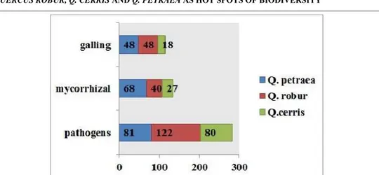
Abstract: Three different bipartite networks (pathogenic, ectomycorrhizal and galling insects) established by Quercus robur L., Q. cerris L. and Q. petraea (Matt.) Liebl. were merged in order to investigate the topological properties of the complex network, shading light on how biodiversity was organized through complex interactions. The complex network contains 290 species – 137 are pathogens (parasitic interaction), 72 are mycorrhizal fungi (mutualists) and 81 species of galling insects (herbivores). Most relevant network descriptors, connectivity, nestedness and modularity were analyzed. The main network and subnetworks displayed different behaviors in terms of topological properties, three of four networks showing significant modularity (galling insects network was marginally significant in what regards modularity). High connectivity and different degrees of nestednesscharacterized all networks. Clustering and Non Metric Multidimensional scaling refined the information provided by network analysis showing that networks occupy distant positions in ordination space and there are differences in terms of resemblance patterns.
Key words: biodiversity, community assembly, composite bipartite network, modularity, nestedness, subnetworks.
Introduction
One of the recurrent questions in ecology, why are there so many species, an inspiring interrogation since the seminal paper of G. E. HUTCHINSON (1959) is still in the quest of a conclusive answer. The answer is not simple and there are only partial explanations for the phenomenon of biodiversity. However, a common ground for investigation lies in the assembly rules which govern the structure of communities and ecosystems [GÖTZENBERGER & al. 2011] and in the structure itself. There is an obvious link between biodiversity as system property [HOLLAND, 1995] and the functioning of the system [LEVIN, 1998].
Network theory provides tools for the analysis of complex networks, ecological networks included [STROGATZ, 2001]. These tools permit the analysis of links simultaneously across the whole network. In a larger context, ecological networks incorporate interaction networks (established by antagonistic and mutualistic interactions, facilitation included) and spatial networks (such as habitat structure at landscape and meta-ecosystem levels), being complex real world networks with a specific small world and scale free topology [BARABÁSI & REKA, 1999; DUNNE & al. 2003; WATTS & STROGATZ, 1998]. Network approach facilitates the description of complex interactions summarized by large matrices, providing insight into ecological processes such as species co-existence, biogeographic frameworks, vulnerability to invasion or to extinction, population genetics and also, mechanisms of biodiversity patterns [ECONOMO & KEITT, 2008; THÉBAULT &
1 University of Oradea, Faculty of Environmental Protection, Forestry and Forest Engineering Department, 26 General Magheru Bld., Bihor County, Oradea – Romania
FONTAINE, 2010; SIMARD & al. 2012; BAHRAM & al. 2014]. From a different perspective, species interaction diversity is analogous to species diversity in its simplest form, as interaction richness with characteristic network properties added [TYLIANAKIS & al. 2010].
Ecological networks depicting species interactions display non-random structure that allows them to persist despite their complexity [BASCOMPTE, 2010] however, the assembly of species within webs is modeled by deterministic and stochastic events which must be considered in the assessment of community structure [GÖTZENBERGER & al. 2011]. Network architecture is described by four main properties: number of nodes, connectance which describes the relative number of interactions, nestedness which describes the level of sharing of interaction patterns among species and modularity showing the degree of compartmentalization of the network [THÉBAULT & FONTAINE, 2010].
Species interactions are generally depicted by unipartite (trophic) and bipartite graphs (depicting mutualistic or antagonistic interactions). Bipartite networks are graphs with constrained wiring, with links between two groups of species, but not within each group. The two distinct sets of species are linked through coevolution and, the bipartite graph captures the main properties of the coevolved interactions such as asymmetry and modularity [JORDANO, 2010]. Intimate interactions established by symbiotic organisms (mutualistic or antagonistic) build networks of different pattern and structure as compared to free living organisms such as consumers and their prey [THOMPSON, 2005]. Being more specialized, networks integrating symbiotic organisms and their hosts display low modularity [PIRES & GUIMARÃES, 2013] and high nestedness [BASCOMPTE & al. 2003; FORTUNA & al. 2010]. It is generally accepted that low intimacy interactions which define consumers and their prey (consumption of plant tissue included), generate networks of different architecture, with high modularity and low nestedness. Connectance, as traditional network topology measure is dependent on species richness (higher in small networks) but has particular signature in trophic and mutualistic networks, with consumers’ network being less connected than mutualistic network [THÉBAULT & FONTAINE, 2010].
Network analysis does not exclude multivariate analysis as traditional class of analytic tools but offers a new perspective and complements it [MELLO & al. 2011], with multivariate analysis focusing on species and network analysis on interactions. Compared to multivariate analysis, networks integrate different aspects including specificity and association breadth [CHAGNON & al. 2012].
Trees are complex organisms in terms of architecture, size, diversity of microhabitats, types of resources and longevity [LAWTON, 1983]. By consequence, biodiversity of associated species from higher trophic levels is vast [TEWS & al. 2004]. Organizing in a meaningful way this type of data becomes an important scientific goal in order to understand why indeed so many species are connected to trees and if trees are biodiversity generators in ecosystems, what consequences will have the unprecedented tree species decline that we witness [BUTCHART & al. 2010].
molecular recognition mechanisms and genetic matching makes this category of highly specialized consumers superficially similar to pathogens. Also they are ideal models for the study of ecological diversity due to their abundance, specificity and richness [PORTUGAL-SANTANA & DOS SANTOS-ISAIAS, 2014].
Trees harbor a vast community of pathogens, the interaction with this category of organisms being antagonistic and the result of the co-evolution process, also intimate, modulated at molecular and genetic level. The impact of herbivores and pathogens on tree diversity was first hypothesized by JANZEN (1970) and CONNELL (1971). This was confirmed experimentally by BAGCHI & al. (2014) who showed that specialized consumers harmed more when their host were abundant, consequently leaving way to the establishment of less competitive tree species and therefore leading to higher biodiversity, at least in tropical areas. On the other hand, these groups of co-evolving organisms include rare parasitic species, mainly wood degrading fungi which are considered reliable indicators of ecosystem’s biodiversity [CHRISTENSEN & al. 2004; ADAMČÍK & al. 2007].
Ectomycorrhizal fungi (ECM) establish beneficial mutualistic relationships with trees, essentially trophic interactions established through co-evolution, with different levels of specificity. There are ECM fungi with broad host range while others colonize few host species or closely related species within one genus [MOLINA & al. 1992; VAN DEN HEIJDEN & al. 2015]. Mycorrhizal interactions only recently were approached in the frame of mutualistic network studies focused more on pollinator and seed dispersal webs [BAHRAM & al. 2014].
The present study addresses the bipartite network properties of three types of communities (pathogens, ectomycorrhizal fungi and galling insects) linked to three important late successional tree species within same genus, dominant in mixed broadleaved forests of North-Western Transylvania, Quercus robur L., Q. cerris L. and Q. petraea (Matt.) Liebl. The summary networks for the three communities were merged in one complex network in order to investigate the topology and properties of the emerged network, assessing the contribution of each subnetwork. The assembly of the three communities was devised to highlight interaction diversity on taxonomically resolved networks. Combined with the information provided by the alternate multivariate analysis, it permits the analysis of possible assembly rule governing the association of different tree dependent communities and is an indirect indication of the importance of tree species as biodiversity key species.
Materials and methods
Compilation of species lists
The bipartite network approach in the case of galling insects which are linked to trees as consumers (traditionally included in unipartite trophic webs) was preferred due to the particular intimate nature of interaction resembling host-pathogen association.
Q. cerris, Q. robur and Q. petraea co-occur in forests located in hilly regions of North Western Transylvania, but our observations are restricted to areas in the proximity of cities as Cluj-Napoca and Oradea, in pure or mixed stands. As dominant, late stage species.
Q robur and Q. petraea are closely related species, hybridizing frequently [SAMUEL & al. 1995; JENSEN & al. 2009], sharing many common features and being sympatric in most of their areal [ELLENBERG, 2009]. Q. cerris is more tolerant to drought, a feature correlated with its’ predominantly southern distribution in Europe and Asia minor, more restricted than
Q. robur and Q. petraea and expected to extend toward North due to the climate change [HLÁSNY & al. 2011].
ECM fungi inventory was based almost exclusively on aboveground observations on EC fungi fructifications over the last 20 years in mixed broadleaved forests in hilly areas of North Western Transylvania, on Q. robur, Q. cerris and Q. petraea, with the exception of
Coenococcum geophilum observed on detached metabolically active roots of the investigated host species. The link to a specific host was assessed by the attachment of the sporophore to the root system. The long period of field observations suggests that at least most important and frequent active mycobionts were assessed but molecular data are needed to cover completely the diversity of ectomycorrhizal fungi [BAHRAM & al. 2014].
Observations on pathogenic, sapro-parasitic and parasitic fungi were gathered over the same extended period, within same types of ecosystems. Galling insects were inventoried beginning with 2006, within same locations.
The nomenclature of ectomycorrhizal fungi and pathogens follows Index Fungorum [www.indexfungorum.org], Global Biodiversity Information and Mycobank [www.mycobank.org]. For galling insects, nomenclature follows Fauna Europaea [www.faunaeur.org] and Melika (2006).
Network analysis
The complex network and separately, galling insects, pathogens and ECM fungi subnetworks were generated in Pajek ver.4.09 [BATAGELJ & MRVAR, 1998] using Kamada-Kawai layout. Unipartite versions of bipartite networks were also generated in Pajek.
Network metrics were calculated using several software packages for better significance testing, since different software authors provided different significance testing methods. Small networks (below 1000 nodes) are characterized by unstable metrics, a problem that arises when using iterative algorithms as in the case of the calculation of modularity and nestedness indices. In fact, many indices are affected by network size [OLESEN & al. 2007] and in the search of most stable results, using different software is helpful.
Network size is the product of total number of interacting species, more precisely the product between the number of hosts and number of their interaction partners, consumers or/and mutualists.
Connectance is a second order property of the network being related to specialization [DORMANN & al. 2009]. Is the proportion of realized interactions from all possible interactions in the network [MAY, 1972]. In bipartite webs it is measured as:
J I
L C
Where: J stands for lower trophic level species and I for higher trophic level species.
Web asymmetry is a simple measure of the balance between the lower (J) and higher trophic (I) level in bipartite networks [DORMANN & al. 2009].
I J I J W
Positive numbers indicate higher trophic level species while negative numbers indicate lower trophic level species prevalence. The index scales within the interval [-1; 1]. When there are more species in the higher trophic level set, the value approaches -1.
Modularity is a network property measuring the tendency of groups of nodes (species) to interact more strongly among themselves than with other nodes in the network, compartmentalization defining the real world networks as opposed to random networks lacking this property [BARABÁSI, 2016; BASCOMPTE, 2010]. Detection of communities in networks is considered to reveal links between topologies and functional traits of biological systems and is considered to be more obvious in antagonistic than in mutualistic networks [OLESEN & al. 2007]. There are many algorithms proposed to search and measure modularity. We chose Louvain algorithm [BLONDEL & al. 2008] (provided by the software Pajek) which estimated the modularity index (Q) using a greedy optimization algorithm. It is the same Newman - Girvan (2004) metric which incorporates hierarchy in successive community search iterations. The optimization is performed in two steps: first it optimizes the modularity locally by clustering the neighboring nodes and during the second phase clusters are aggregated until modularity ceases to increase.
NMi j i i E R k C k E E Q 1 2
Where: kiC represents the sum of degrees of nodes within module i that belong to set C and
kjR represents the sum of degrees of nodes within module i that belong to set R; Ei represents the number of links in module i; E the number of links in the complete network.
The partition of nodes that gives rise to the maximum Q value is considered as community structure of a graph or network. Modularity index quantifies the degree of modules’ clear delimitation [OLESEN & al. 2007].
The results are considered to be robust and comparable to simulated annealing results [POISOT & al. 2013]. We used the default settings of the algorithm: resolution parameter set to 1, number of random restarts was 5, maximum number levels at each iteration - 20 and the number of repetitions at each level set to 50. The algorithm was repeated 50 times until a stable number of modules and of modularity value was obtained.
For comparisons, NETCARTO software [GUIMERÀ & AMARAL, 2005] was employed. The metric used for the present study was the most popular with modularity analysis, Q metric of Girvan and Newman (2002). Guimerà and Amaral (2005) developed an algorithm for modularity optimization over possible partitions by using simulated annealing. Significance testing is performed according to null model III, number of links in random models is the same with number of links in observed network reproducing in this way the real data [GOTELLI, 2000].
scores, which use the empirical modularity, value Qcalc, mean and standard deviation of simulated matrices’ modularity [GUIMERÀ & al. 2004]. Significant modularity implies z ≥1.
Z= (Qcalc-μ)/σ
The roles and degree of connectivity of each node can be assessed in parameter z-P space (P standing for participation coefficient which measures how well are distributed the links of node i among modules and z for within module degree, which measures how well is connected node i to other nodes in module). Nodes are classified in this space as non-hub and hub nodes while non-hub nodes can play different roles as: ultra-peripheral, peripheral, connector and kinless nodes [GUIMERÀ & AMARAL, 2005].
Nestedness is a presence-absence matrix property displayed also by the corresponding matrix quantified by an index which is the measure of how much of the matrix elements can be packed without holes [ARAUJO & al. 2010]. In nested matrices, specialist species interact with generalists hosts. The concept was first used in biogeographic context to explain the diversity pattern of species from poor sites as being subsets of species rich sites [ATMAR & PATTERSON, 1993] and became a key tool to characterize network structure [ARAUJO & al. 2010]. To calculate matrix temperature, the authors used an analogy from thermodynamics, characterizing matrix order as 0°C temperature and complete disorder as 100°C. At zero degrees temperature, a thermodynamic system presents particles in the state of minimal energy analogous to a completely nested structure while, in the state of complete disorder particles present high energy level analogous to a non-nested matrix. Nestedness is calculated as N=(100-T)/100, [BASCOMPTE & al. 2003], N being defined in the range [0,1] where 1 corresponds to a perfectly nested network and 0 corresponds to systems where interactions occur completely at random. Matrix temperature was calculated using BINMATNEST software [RODRÍGUEZ-GIRONÉS & SANTAMARÍA, 2006] using 100 randomizations for significance testing. We employed also results yielded by the package
bipartite for R [DORMANN & al. 2008].
Different software use different null models to test significance of the results: the actual network against a randomly assembled network under more or less liberal restrictions. BINMATNEST provides the results of testing null models I, II and III but authors recommend to use as benchmark, null model III (FE-fixed row totals and equiprobable column totals) [ULRICH & GOTELLI, 2007]. R bipartite package employs null model r00 or null model I, the most liberal of null models assuming that column and row total vary freely. The alternative hypothesis states that observed statistic is greater or less than simulated statistic (1000 simulations). Alternative significance testing is provided by SES (Standardized Effect Size) which measures the number of standard deviations that the observed statistic is above or below the mean statistic of simulated null matrices. SES above 2 and below -2 indicates significant result at error level of 5% [ULRICH & GOTELLI, 2007].
Classical community analysis approach
To test the level of pattern detection provided by network analysis we employed classical community analysis methods such as cluster analysis and Non Metric Multidimensional Scaling (NMDS).
Clustering is an exploratory method of grouping entities (species) according to a resemblance measure. Clustering was performed using UPGMA (Unweighted Pair Group Method with Arithmetic Mean) algorithm and as dissimilarity measure, Euclidean distance. The graphical representation, the dendrogram records the sequences of merges of entities, for instance species, and splits which generate groups. The species are compared pairwise.
Clustering depends highly on the similarity measure used: one robust measure is Euclidean distance [HAMMER & al. 2001] which we employed in our cluster analysis.
We tested for correlation between similarity matrices of the three categories of organisms and also between the complex matrix and each of the categories using Mantel test [MANTEL, 1967]. Mantel test analyzes the correlation between 2 distance matrices being a non-parametric significance test. It computes the significance of correlation through permutation of rows and columns of the input matrices. The test statistic is Pearson product moment, R coefficient taking values in the [-1:1] range.
Non-metric Multidimensional Scaling ranks distances among objects and uses the ranks to map the objects onto two-dimensional ordination space preserving the ranked differences [SHEPARD, 1966] and operating in most parsimonious way. The essence of the method consists in finding the configuration of points compatible with a given dissimilarity relation among them permitting the visualization of a structure hidden in the original data [KENKEL & ORLÓCI, 1986; BORG & GROENEN, 2005]. The method is iterative and several iterations are performed until the lowest stress value (the best goodness of fit) is obtained. The proximity among objects in the ordination space corresponds to their similarity. We used Euclidean distance as similarity measure.
Clustering and NMDS were performed using software PAST [HAMMER & al. 2001].
Results
Interaction matrix
Tab 1.Matrix of pathogenic, ectomycorrhizal and galling insects’ species associated to host trees
Nr.12 Nr.23 Species Q.
robur Q. cerris
Q. petraea Pathogens
1. 1. Abortiporus biennis (Bull.) Singer 1 1 1
2. 2. Aleurodiscus disciformis (DC.) Pat. 1 1 1
3. 3. Aleurodiscus oakesii (Berk. & M. A. Curtis) Cooke 1 0 1
4. 4. Alternaria alternata (Fr.) Keissl. 1 1 1
5. 5. Amphiporthe leiphaemia (Fr.) Butin 1 1 1
6. 6. Anthostoma decipiens (DC.) Nitschke 1 1 0
7. 7. Antrodia albida (Fr.) Donk 1 1 1
8. 8. Antrodiella semisupina (Berk. & M. A. Curtis) Ryvarden 1 1 0 9. 9. Apiocarpella quercicola Tak. Kobay. & K. Sasaki 1 0 0 10. 10. Apiognomonia errabunda (Roberge ex Desm.) Höhn 1 1 1
11. 11. Armillaria gallica Marxm. & Romagn. 1 1 0
12. 12. Armillaria mellea (Vahl) P. Kumm. 1 1 1
13. 13. Armillaria tabescens (Scop.) Emel 1 1 1
14. 14. Ascochyta quercus Sacc. & Speg., 1 1 1
15. 15. Aureobasidium apocryptum (Ellis & Everh.) Herm.-Nijh 1 0 0
16. 16. Bjerkandera adusta (Willd.) P. Karst. 1 0 0
17. 17. Botryodiplodia sp. 1 0 0
18. 18. Botryosphaeria stevensii Shoemaker 1 1 0
19. 19. Botryotinia fuckeliana (de Bary) Whetzel 1 1 1
20. 20. Buglossoporus pulvinus (Pers.) Donk 1 1 1
21. 21. Cerrena unicolor (Bull.: Fr.) Murrill 1 1 1
22. 22. Chondrostereum purpureum (Pers.) Pouzar 1 0 1
23. 23. Ciboria batschiana (Zopf) N. F. Buchw 1 0 1
24. 24. Colpoma quercina (Pers.) Wahll. 1 1 0
25. 25. Cryphonectria parasitica (Murrill) M. E. Barr 1 0 1
26. 26. Cryptocline cinerascens (Bubák) Arx 1 1 1
27. 27. Daedalea quercina (L.) Pers. 1 1 1
28. 28. Daldinia childiae J. D. Rogers & Y. M. Ju 1 0 0
29. 29. Diaporthe insularis Nitschke 1 0 1
30. 30. Diatrypella quercina (Pers.) Cooke 1 1 1
31. 31. Dicarpella dryina Belisario & M. E. Barr 1 1 0 32. 32. Diplodia corticola A. J. L. Phillips, A. Alves & J. Luque 0 1 1 33. 33. Diplogelasinospora grovesii Udagawa & Y. Horie 0 0 1
34. 34. Elsinoe quercicola Bitanc. & Jenkins 1 0 0
35. 35. Entonaema cinnabarinum (Cooke & Massee) Lloyd 1 0 0
36. 36. Erwinia herbicola (Lohnis 1911) Dye 0 1 0
37. 37. Erysiphe alphitoides (Griffon & Maubl.) U. Braun & S.
Takam. 1 1 1
38. 38. Erysiphe hypophylla (Nevod.) U. Braun & Cunningt. 1 0 1 39. 39. Erysiphe quercicola S. Takam. & U. Braun 1 1 1
40. 40. Eutypa quercicola Berk. 1 1 1
41. 41. Fistulina hepatica (Schaeff.) With. 1 1 1
42. 42. Fomes fomentarius (L.) Fr. 0 0 1
43. 43. Fuscoporia contigua (Pers.) G. Cunn 1 1 0
44. 44. Fuscoporia ferruginosa (Schrad.) Murrill 1 0 0
45. 45. Fuscoporia torulosa (Pers.) T. Wagner & M. Fisch. 1 0 0
46. 46. Fusicoccum quercus Oudem. 1 0 0
2Complex matrix
Nr.12 Nr.23 Species Q.
robur Q. cerris
Q. petraea
47. 47. Ganoderma applanatum (Pers.) Pat. 1 1 1
48. 48. Ganoderma lucidum (Curtis) P. Karst. 1 1 1
49. 49. Gibberella baccata (Wallr.) Sacc. 1 0 0
50. 50. Gibberella pulicaris (Kunze) Sacc. 0 0 1
51. 51. Gibberella zeae (Schwein.) Petch 1 0 0
52. 52. Globisporangium spiculum (B. Paul) Uzuhashi, Tojo &
Kakish 1 0 0
53. 53. Globisporangium ultimum (Trow) Uzuhashi, Tojo &
Kakish. 1 0 0
54. 54. Gnomoniopsis clavulata (Ellis) Sogonov 1 1 1
55. 55. Grifola frondosa (Dicks.) Gray 1 0 1
56. 56. Gymnopus fusipes (Bull.) Gray 1 1 1
57. 57. Hapalopilus croceus (Pers.) Bondartsev et Singer 1 1 1
58. 58. Hapalopilus nidulans (Fr.) P. Karst. 1 1 1
59. 59. Helicomyces roseus Link 0 0 1
60. 60. Hericium cirrhatum (Pers.) Nikol 1 1 1
61. 61. Hericium erinaceus (Bull.) Pers. 1 1 1
62. 62. Hymenochaete rubiginosa (Dicks.) Lév. 1 1 1
63. 63. Hypospilina pustula (Pers.) M. Monod, 1 1 1
64. 64. Inonotus andersonii (Ellis & Everh.) Nikol 1 1 0
65. 65. Inonotus hispidus (Bull.) P. Karst 1 1 1
66. 66. Inonotus nidus-pici Pilat ex Pilat 0 1 0
67. 67. Inonotus obliquus (Ach. ex Pers.) Pilát 1 1 0
68. 68. Inonotus rheades (Pers.) Fiasson & Niemelä 1 1 1
69. 69. Inonotus rickii (Pat.) Reid 0 1 0
70. 70. Irpex mollis Berk. & M.A. Curtis 1 1 1
71. 71. Laetiporus sulphureus (Bull.) Murrill 0 0 1
72. 72. Lentinus arcularius (Batsch) Zmitr 0 1 0
73. 73. Lenzites betulina (L.) Fr. 1 1 1
74. 74. Loranthus europaeus Jacq. 1 1 1
75. 75. Meripilus giganteus (Pers.) P. Karst. 1 0 0
76. 76. Microsphaera silvatica Vlasov 1 0 0
77. 77. Microstroma album (Desm.) Sacc. 1 1 1
78. 78. Monochaetia monochaeta (Desmaz.) Allesch. 1 1 0
79. 79. Mycelium radicis-atrovirens Melin 1 0 0
80. 80. Nemania serpens (Pers.: Fr.) S. F. Gray. 1 0 0
81. 81. Neofusicoccum parvum (Pennycook & Samuels) Crous,
Slippers & A. J. L. Phillips 1 0 0 82. 82. Nodulisporium corticioides(Ferraris & Sacc.) S. Hughes 1 0 0
83. 83. Peniophora quercina (Pers.) Cooke 0 1 0
84. 84. Pesotum piceae J. L. Crane & Schokn 1 1 0
85. 85. Pestalotiopsis monochaeta Maharachch. K. D. Hyde &
Crous 1 0 0
86. 86. Pestalotiopsis neglecta (Thüm.) Steyaert 1 1 1
87. 87. Pezicula cinnamomea (DC.) Sacc 1 0 1
88. 88. Pezicula melanigena (T. Kowalski & Halmschl.) P. R.
Johnst. 1 0 1
89. 89. Phellinopsis conchata (Pers.) Y. C. Dai 1 0 0
90. 90. Phialocephala dimorphospora W. B. Kendr 1 1 0
91. 91. Phlebia radiata Fr. 1 0 0
92. 92. Pholiota squarrosa (Vahl) P. Kumm 1 1 0
93. 93. Phomopsis glandicola (Lév.) Grove 1 0 1
94. 94. Phomopsis quercina (Sacc.) Höhn. ex Died. 1 0 0
Nr.12 Nr.23 Species Q.
robur Q. cerris
Q. petraea 96. 96. Phytophthora plurivora T. Jung & T. I. Burgess 1 0 0 97. 97. Phytophthora cactorum (Lebert & Cohn) J. Schröt. 1 0 0
98. 98. Phytophthora citricola Sawada 1 1 1
99. 99. Phytophthora cryptogea Pethybr. & Laff. 0 1 0
100. 100. Piptoporus quercinus(Schrad.) P. Karst. 1 1 1
101. 101. Podoscypha multizonata (Berk. & Broome) Pat. 1 0 0
102. 102. Polyporus squamosus (Huds.) Fr. 1 0 0
103. 103. Porostereum spadiceum (Pers.) Hjortstam & Ryvarden 1 0 0
104. 104. Postia subcaesia (A. David) Jülich 1 0 1
105. 105. Pseudoinonotus dryadeus (Pers.) T. Wagner & M. Fisch. 1 1 1
106. 106. Pseudomonas quercus Schern 1 0 0
107. 107. Pythium inflatum V. D. Matthews 1 0 1
108. 108. Pythium sterilum Belbahri & Lefort 1 1 1 109. 109. Ramularia endophylla Verkley & U. Braun 1 0 0 110. 110. Rigidoporus lineatus (Pers.) Ryvarden 1 0 0
111. 111. Rosellinia necatrix Berl. ex Prill. 1 1 1
112. 112. Schizophyllum commune Fr. 1 1 1
113. 113. Schizopora paradoxa (Schrad.) Donk 0 1 1
114. 114. Septoria quercicola Sacc. 1 0 0
115. 115. Spongipellis litschaueri Lohwag 1 1 1
116. 116. Spongipellis spumeus (Sowerby) Pat 1 1 1
117. 117. Steccherinum ochraceum (Pers.) Gray 1 0 1
118. 118. Stereum gausapatum (Fr.) Fr. 1 1 1
119. 119. Stereum hirsutum (Willd.) Pers. 1 1 1
120. 120. Stereum ochraceoflavum (Schwein.) Sacc. 1 1 1
121. 121. Stereum rameale (Schwein.) Burt 1 0 1
122. 122. Stereum rugosum Fr. 1 0 0
123. 123. Stereum subtomentosum Pouzar 1 0 1
124. 124. Taphrina coerulescens (Desm. & Mont.) Tul. 0 1 0
125. 125. Trametes hirsuta (Wulfen) Lloyd 1 1 1
126. 126. Trametes trogii Berk 1 0 1
127. 127. Trametes versicolor (L.) Lloyd 1 1 1
128. 128. Tyromyces fissilis (Berk. & Curt.) Donk 1 1 1
129. 129. Valsa intermedia Nitschke 1 0 1
130. 130. Verticillium dahliae Kleb. 0 1 1
131. 131. Viscum album L. 1 1 1
132. 132. Vuilleminia comedens (Nees.) Maire 1 1 1
133. 133. Vuilleminia cystidiata Parmasto 1 1 1
134. 134. Vuilleminia megalospora Bres 1 1 1
135. 135. Xanthomonas campestris (Pammel, 1895) Dowson, 1939 1 1 0 136. 136. Xylebolus frustulatus (Berk & M. A. Curtis) Boidin 1 1 1 137. 137. Xylobolus subpileatus (Berk. & M. A. Curtis) Boidin 1 1 0
Ectomycorrhizal fungi
138. 1. Coenococcum geophilum Fr. 1 1 1
139. 2. Lactarius circellatus (Battara) Fr. 1 1 1
140. 3. Amanita rubescens (Pers.:Fr.) Gray 1 1 1
141. 4. Amanita phalloides (Vaill. ex Fr.) Link 0 0 1
142. 5. Russula foetens (Pers.) Pers. 1 1 1
143. 6. Russula cyanoxantha (Schaeff.) Fr. 1 1 1
144. 7. Lactarius quietus (Fr.) Fr. 0 0 1
145. 8. Russula fragilis sensu Cooke 0 0 1
146. 9. Lactarius vellereus (Fr.) Fr. 1 0 1
Nr.12 Nr.23 Species Q.
robur Q. cerris
Q. petraea
148. 11. Xerocomellus chrysenteron (Bull.) Šutara 1 1 1
149. 12. Butyriboletus appendiculatus (Schaeff.) O. A. Arora & J. J.
Frank 1 1 1
150. 13. Xerocomellus porosporus (Imler ex. Bon) Šutara 1 0 1
151. 14. Russula nobilis Velen. 0 0 1
152. 15. Russula consobrina (Fr.) Fr. 0 0 1
153. 16. Boletus reticulatus Schaeff. 1 1 1 154. 17. Suillellusqueletii (Schulzer) Vizzini, Simonini & Gelardi 0 0 1 155. 18. Suillellus luridus (Schaeff.) Murrill 1 1 1
156. 19. Gyroporus castaneus (Bull.) Quél. 0 0 1
157. 20. Lactarius piperatus (L.) Pers. 1 1 1
158. 21. Lactarius volemus (Fr.) Fr. 0 0 1
159. 22. Craterellus cornucopioides (L.) Pers. 1 1 1
160. 23. Inocybe rimosa (Bull.) P. Kumm. 1 1 1
161. 24. Scleroderma citrinum Pers. 1 1 1
162. 25. Russula cessans A. Pearson 0 0 1
163. 26. Boletus subtomentosus L. 0 0 1
164. 27. Amanita vaginata (Bull.) Lam. 1 1 1
165. 28. Russula virescens (Schaeff.) Fr. 1 0 1
166. 29. Tricholoma saponaceum (Fr.) P. Kumm. 1 0 1
167. 30. Russula claroflava Grove 1 0 1
168. 31. Russula fellea (Fr.) Fr. 1 0 0
169. 32. Hygrophorus eburneus (Bull.) Fr. 0 0 1
170. 33. Russula vesca Fr. 1 0 1
171. 34. Laccaria laccata (Scop.) Cooke 1 1 1
172. 35. Laccaria amethystina (Huds.) Cooke 1 0 1
173. 36. Hebeloma crustuliniforme (Bull.) Quél. 1 1 1
174. 37. Russula pectinatoides Peck 0 0 1
175. 38. Suillellus satanas (Lenz) Blanco-Dios 1 1 0
176. 39. Cortinarius sp. 0 0 1
177. 40. Amanita lividopallescens (Secr. ex Boud.) Kühner &
Romagn 0 0 1
178. 41. Russula rosea Pers. 0 0 1
179. 42. Russula parazurea Jul. Schäff. 1 0 1
180. 43. Paxillus involutus (Batsch) Fr. 1 0 1
181. 44. Inocybe sp. 0 1 1
182. 45. Tricholoma virgatum (Fr.) P. Kumm. 1 0 1
183. 46. Leccinum aurantiacum (Bull.) Gray 0 0 1
184. 47. Russula nigricans Fr. 1 1 1
185. 48. Lactarius chrysorrhaeus Fr. 0 0 1
186. 49. Lactarius camphoratus (Bull.) Fr. 0 0 1
187. 50. Amanita echinocephala (Vittad.) Quél. 0 0 1
188. 51. Russula romellii Maire 0 1 1
189. 52. Russula ionochlora Romagn. 0 1 1
190. 53. Russula atropurpurea (Krombh.) Britzelm. 1 0 0
191. 54. Amanita virosa Bertill. 1 0 1
192. 55. Amanita ceciliae (Berk. & Broome) Bas. 0 0 1 193. 56. Amanita pantherina sensu Gonnermann & Rabenhorst 1 1 1
194. 57. Lactarius fulvissimus Romagn. 0 0 1
195. 58. Russula brunneoviolacea Crawshay 0 0 1
196. 59. Scleroderma areolatum Pers. 1 0 1
197. 60. Hemileccinum impolitum (Fr.) Šutara 0 0 1
198. 61. Russula viridicans Carteret & Reumaux 0 0 1
Nr.12 Nr.23 Species Q.
robur Q. cerris
Q. petraea
200. 63. Ramaria stricta (Pers.) Quél. 1 1 1
201. 64. Lactarius blennius (Fr.) Fr. 0 0 1
202. 65. Russula aurea Pers. 0 0 1
203. 66. Cyanoboletus pulverulentus (Opat.) Gelardi, Vizzini &
Simonini 0 0 1
204. 67. Russula decolorans (Fr.) Fr. 0 0 1
205. 68. Lactarius scrobiculatus (Scop.) Fr. 0 0 1
206. 69. Suillus granulatus (L.) Roussel 1 0 1
207. 70. Russula grata Britzelm. 1 1 1
208. 71. Boletus edulis Bull. 1 1 0
209. 72. Entoloma sinuatum (Bull.) P. Kumm. 1 1 1
Galling insects
210. 1. Andricus lucidus (= A. aestivalis Giraud, 1859 ♀♂) 0 1 0
211. 2. Andricus amblycerus Giraud, 1859 ♀ 1 0 1
212. 3. Andricusaries Giraud, 1859 ♀ 1 0 0
213. 4. Andricus autumnalis Mayr, 1882 ♀♀ 0 0 1
214. 5. Andricus caliciformis Giraud, 1859 ♀ 1 0 1
215. 6. Andricus callidoma (= A. cirratus Adler, 1881 ♀♂) 1 0 0
216. 7. Andricus callidoma Hartig, 1841 ♀♀ 0 0 1
217. 8. Andricus collaris Hartig, 1840 ♀♀ 1 0 1 218. 9. Andricus collaris (= A. curvator Hartig, 1840 ♀♂) 1 0 1
219. 10. Andricus conglomeratus Giraud, 1859 ♀ 0 0 1
220. 11. Andricus coriarius Hartig, 1843 ♀ 1 0 1
221. 12. Andricus corruptrix Schlechtendal, 1870 ♀♀ 1 0 1
222. 13. Andricus crispator Tschek, 1871 ♀♀ 0 1 0
223. 14. Andricus cydoniae Giraud, 1859 ♀♂ 0 1 0
224. 15. Andricus foecundatrix Hartig, 1840 ♀♀ 1 0 0
225. 16. Andricus galeatus Giraud, 1859 ♀ 0 0 1
226. 17. Andricus gallaetinctoriae Olivier, 1791 ♀♀ 1 0 1
227. 18. Andricus gemmeus Giraud, 1859 ♀♀ 1 0 1
228. 19. Andricus gemmeus Giraud, 1859 ♀♂ 0 1 0
229. 20. Andricus glandulae Hartig, 1840 ♀ 0 0 1
230. 21. Andricus glutinosus Giraud, 1859 ♀ 1 0 1
231. 22. Andricus grossulariae (= A. mayri Mayr, 1882 ♀♀) 1 0 0 232. 23. Andricus grossulariae (= A. grossulariae Giraud, 1859 ♀♂) 1 0 0
233. 24. Andricus inflator Hartig, 1840 ♀♀ 1 0 1
234. 25. Andricus inflator (= Cynips globuli Hartig, 1840 ♀♂) 1 0 0 235. 26. Andricus kollari Hartig, 1843 ♀♀ 1 0 1
236. 27. Andricus lignicolus Hartig, 1840 ♀♀ 1 0 1
237. 28. Andricus lucidus Hartig, 1843 ♀♀ 1 0 1
238. 29. Andricus malpighii Adler, 1881 ♀♀ 0 0 1
239. 30. Andricus mitratus Mayr, 1870 ♀ 0 0 1
240. 31. Andricus multiplicatus Giraud, 1859 ♀♂ 0 1 0
241. 32. Andricus paradoxus Radoszkowski, 1866 ♀♀ 1 0 1
242. 33. Andricus polycerus Giraud, 1859 ♀ 0 0 1
243. 34. Andricus quadrilineatus Hartig, 1840 ♀♀ 1 0 0
244. 35. Andricus quercuscalicis Burgsdorff, 1783 ♀♀ 1 0 0 245. 36. Andricus quercuscorticis Linnaeus, 1761 ♀♀ 0 0 1 246. 37. Andricus quercusradicis Fabricius, 1798 ♀♀ 1 0 1 247. 38. Andricus quercusradicis (A. trilineatus Hartig, 1840 ♀♂) 1 0 1
248. 39. Andricus schroeckingeri Wachtl, 1876 ♀ 1 0 1
249. 40. Andricus seminationis Giraud, 1859 ♀ 1 0 0
250. 41. Andricus serotinus Giraud, 1859 ♀ 0 0 1
Nr.12 Nr.23 Species Q.
robur Q. cerris
Q. petraea
252. 43. Andricus seckendorffi Wachtl, 1879 0 0 1
253. 44. Andricus gallaeurnaeformis (= A. sufflator Mayr, 1882
♀♂) 1 0 0
254. 45. Andricus superfetationis Giraud, 1859 ♀ 1 0 0
255. 46. Andricus testaceipes Hartig, 1840 ♀♀ 1 0 0
256. 47. Andricus testaceipes Hartig, 1840 ♀♂ 1 0 0
257. 48. Andricus truncicola Giraud, 1859 ♀ 1 0 1
258. 49. Andricus vindobonensis Müllner, 1901 ♀♂ 0 1 0
259. 50. Aphelonyx cerricola Giraud, 1859 ♀ 0 1 0
260. 51. Biorhiza pallida Olivier, 1791 ♀♂ 1 0 1
261. 52. Chilaspis nitida (= C. lowi Wachtl, 1882 ♀♂) 0 1 1
262. 53. Chilaspis nitida Giraud, 1859 ♀♀ 0 1 0
263. 54. Contarinia quercicola Rubsaamen, 1899 0 1 0
264. 55. Cynips agama Hartig, 1840 ♀♀ 1 0 1
265. 56. Cynips disticha Hartig, 1840 ♀♀ 1 0 1
266. 57. Cynips divisa Hartig, 1840♀♀ 1 0 1
267. 58. Cynips longiventris Hartig, 1840 ♀♀ 1 0 0
268. 59. Cynips quercusfolii (= C. taschenbergi Schlechtendal,
1870 ♀♂) 0 0 1
269. 60. Cynips quercusfolii Linnaeus, 1758 ♀♀ 1 0 1
270. 61. Trigonaspis megaptera (= Cynips renum Hartig, 1840 ♀♂) 0 0 1
271. 62. Dryomyia circinans Giraud, 1861 0 1 0
272. 63. Epinotia festivana Hübner, 1799 0 0 1
273. 64. Heliozela sericella Haworth, 1828 1 0 1
274. 65. Janetia nervicola Kieffer, 1909 0 1 0
275. 66. Macrodiplosis pustularis Bremi, 1847 1 0 1
276. 67. Macrodiplosis roboris Hardy, 1854 1 0 1
277. 68. Neuroterus anthracinus Curtis, 1838 ♀♀ 1 0 1
278. 69. Neuroterus lanuginosus Giraud, 1859 ♀ 0 1 0
279. 70. Neuroterus quercusbaccarum (= Diplolepis lenticularis
Olivier, 1791 ♀♂) 1 0 1
280. 71. Neuroterus minutulus Giraud, 1859 ♀ 0 1 0
281. 72. Neuroterus numismalis Fourcroy, 1785 ♀♀ 1 0 0
282. 73. Neuroterus numismalis (= N. vesicatrix Schlechtendal,
1870 ♀♂) 1 0 1
283. 74. Neuroterus politus Hartig, 1840 ♀♂ 1 0 1
284. 75. Neuroterus quercusbaccarum Linnaeus, 1758 ♀♀ 1 0 1
285. 76. Neuroterus saliens Kollar, 1857 ♀♀ 0 1 0
286. 77. Polystepha malpighi Kieffer, 1909 0 0 1
287. 78. Pseudoneuroterus macropterus Hartig, 1843 ♀ 0 1 0
288. 79. Synophrus pilulae Houard, 1911 0 1 0
289. 80. Synophrus politus Hartig, 1843 0 1 0
Fig. 1. The repartition of galling insects, tree pathogens and ECM fungi according to the hosts.
Network analysis
Networks are characterized by high asymmetry caused by high number of associated higher trophic level species (network size = 870). The complex network (Fig. 2) shows the highest level of asymmetry, followed by tree pathogens network, and galling insects together with ECM fungi with very close asymmetry values (Tab. 2).
Fig. 2. Bipartite complex network and subnetworks: the radius of nodes is proportional to weighted node
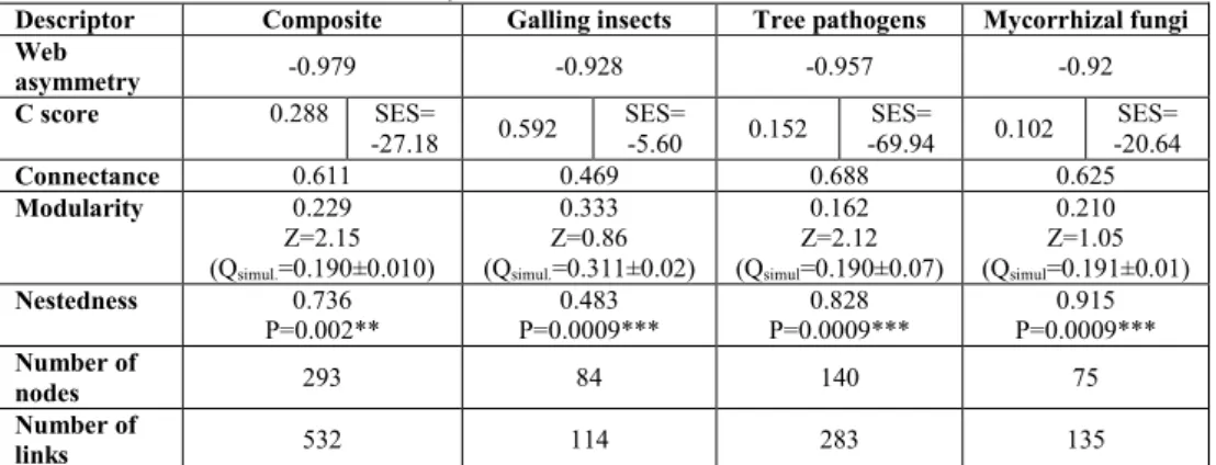
Tab. 2. Nestedness results provided by package bipartite in R. Modularity results produced by software MODULAR with significance expressed in z score values (z scores ≥1, not significant
result). C score estimated in EcoSim.
Descriptor Composite Galling insects Tree pathogens Mycorrhizal fungi Web
asymmetry -0.979 -0.928 -0.957 -0.92
C score 0.288 SES=
-27.18 0.592
SES=
-5.60 0.152
SES=
-69.94 0.102
SES= -20.64
Connectance 0.611 0.469 0.688 0.625
Modularity 0.229
Z=2.15 (Qsimul.=0.190±0.010)
0.333 Z=0.86 (Qsimul.=0.311±0.02)
0.162 Z=2.12 (Qsimul=0.190±0.07)
0.210 Z=1.05 (Qsimul=0.191±0.01)
Nestedness 0.736
P=0.002**
0.483 P=0.0009***
0.828 P=0.0009***
0.915 P=0.0009*** Number of
nodes 293 84 140 75
Number of
links 532 114 283 135
Note: *significant at p<0.05; **significant at p<0.01; ***significant at p<0.001
The complex network and subnetworks are highly connected, lowest connectance characterizing galling insects subnetwork, the most host specialized organisms included in this study and herbivorous consumers, a pattern observed also elsewhere [THÉBAULT & FONTAINE, 2010].
For each network (complex and subnetworks) we ran the modularity detecting algorithm SA (simulated annealing) in MODULAR and NETCARTO and Louvain method in Pajek. All employed software produced same modularity indices but with different significance levels. According to significance testing using z scores, all networks were significantly modular (z scores ≥1), except for galling insects network (Tab. 2 reports the NETCARTO results).
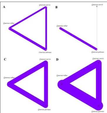
The unipartite versions of the networks (Fig. 3) illustrate de level of species sharing among hosts, this display suggesting niche overlap [MELLO & al. 2011]. Lowest overlap is observed in galling insects and the highest in complex and pathogenic networks. Host specialization is greater in galling insects than in other associated species, a feature that explains differences in sharing pattern.
A rule of a thumb indicates that modularity refers to the situation with more links within modules than outside the modules and this situation is depicted in P-z space [GUIMERÀ & AMARAL, 2005] by assigning to nodes different roles. The complex network contains 23% connector nodes, 30% peripheral nodes and 47.58% ultraperipheral nodes (linked to only one host). Pathogenic network displays a similar repartition of node roles: 33.57% are connectors, 29.19% are peripheral nodes and 40.14% are ultraperipheral nodes. Galling insects establish with their hosts a peculiar network, without connectors, 40.24% peripheral nodes and 57.75% ultraperipheral nodes. This repartition of node roles generates an apparently modular network but the lack of connector nodes is causing a defective structure which cannot be tracked as significant. ECM network displays 30.55% connector nodes, 20.83% peripheral nodes and 50% ultraperipheral. All networks contain three module hubs corresponding to tree hosts.
nestedness under the liberal null model I (r00) (results provided by bipartite package of R). Nestedness results are shown in Tab. 2, as provided by R, considering null model r00.
Fig. 3. Unipartite versions of the networks (A – ECM network, B –galling insects’ network,
C – pathogenic network, D – complex network)
The highest C score (Tab. 2) corresponds to galling insects community, apparently assembled by aggregation (indicated by negative SES scores). Same pattern at lower scores is encountered in complex network and the rest of subnetworks. C scores close to 0 however, indicate a pattern close to random suggesting that there is a degree of stochasticity in community assemblages.
Network topologies reflect the phylogenetic closeness among hosts, the number of shared species being high and suggesting large niche overlap in associated species sharing among hosts. The topology of the complex, with mixed interactions network is characterized by high connectance, low modularity and high nestedness, being closer to symbiotic networks pattern. Subnetworks follow the already observed pattern of low modularity for symbionts, higher for consumers, and high nestedness for symbionts, lower for consumers.
Community analysis
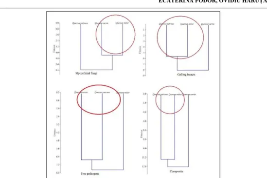
Fig. 4. Dendrograms of clustering pattern in ECM, galling insects’, pathogenic, and complex communities (UPGMA clustering algorithm and Euclidean distance as resemblance measure)
Fig 5. Mapping of ECM, galling insects, pathogenic and complex communities in NMDS ordination
Modularity analysis suggests that there are three significant clusters meaning that a splitting line should be traced above the branching level in dendrograms.
Non Metric Multidimensional Scaling: The mapping of complex community and separate associated to tree hosts organisms’ communities shows consistent differences between the three selected tree hosts in terms of shared communities, in this case the positioning being different for all investigated communities (Fig. 5). For the obtained configurations, minimum stress of 0 corresponds to best agreement between dissimilarity matrices and distances in ordination space (R2 for complex network of 0.9903, for pathogens, 0.9921, for mycorrhizal fungi 0.9934 and for galling insects, 0.9997). The analysis of the resemblance matrix using NMDS highlighted more subtle differences among analyzed communities, a feature confirmed by Mantel tests (resemblance matrices were not significantly correlated).
Discussion
The evolution of plants in terrestrial environments triggered the evolution of various groups of associated organisms by species interactions, trophic webs and diversification of available niches. Closely related hosts tend to share many of their interaction partners, even more if they co-exist in the same geographic area or even location. All the interactions of the three categories of organisms presented in this study merged in one complex network are intimate, resource oriented.
The three functional groups of organisms affect tree hosts modifying the level of productivity and their fitness, hosts in turn present as functional trait susceptibility to herbivory and to pathogens/mutualists. The consumption/mutualistic interaction and susceptibility of hosts are community level traits affecting the ecosystem functions (productivity, nutrient cycling) and structure (habitat optimization via mutualistic interactions) [MATTHEWS & al. 2011]. The very same traits are responsible for the assemblage of associated communities.
The diversity of merged summary network revealed the fact that the number of species using trees is impressive. As networks are open structures, the attachment of new nodes and links covering other types of interactions (other categories of consumers, enemies of herbivorous insects, fungal endophytes, corticolous lichens, etc.) could increase consistently the size of the network.
The networks reflect the phylogenetic closeness of hosts and also the differences in their ecology. Q cerris is clearly separated from Q. petraea and Q. robur in terms of biogeographic range (confined more to Central and Southern Europe, also to Asia Minor) and fundamental niche (in terms of tolerance to drought and ability to vegetate on different types of soil, etc.) [ELLENBERG, 2009]. Dependent species assemblages (ECM, galling insects and pathogens) on Q. cerris are more dissimilar to the other two Quercus species (at greater extent observed for galling insects and the complex network).
linked to lower specialization [POISOT & GRAVEL, 2014], differences among hosts being small in terms of resource type use.
Connectance as network first order property is the result of co-evolution [PETANIDOU & POTTS, 2006; POISOT & GRAVEL, 2014] and the lower the connectance, the higher is the specialization, a structural feature observed in parasitic networks [BELLAY & al. 2013], applied also to pathogenic network under study. Higher diversity and connectance promotes stability in mutualistic networks and destabilize trophic networks (based on free living consumers) [THÉBAULT & FONTAINE, 2010]. However, small networks are characterized by default by high connectance [THÉBAULT & FONTAINE, 2010], a rule applying to our data as well.
Modularity is linked to ecosystem stability and co-evolution [OLESEN & al. 2007]. The striking result of low-modular structure of the investigated networks has an explanation found in the evolution of other biological systems such as genomes, showing that modular structures are usually less optimal than non-modular [KASHTAN & ALON, 2005]. Authors have shown that modularity evolves spontaneously in biological systems and causes emergent properties: stability, robustness under changing environment pressures because designs including modularity manifest higher survival rates. Modularity requires at least networks of 150 nodes to be significantly non-random [OLESEN & al. 2007]. Closely related hosts on the other hand share many of their associated species. As modularity evolves as a response to changes in environment, closely related hosts adapt in a correlative way. When several hosts from distantly related genera are used to construct the network (considering mycorrhizal species or pathogens), modularity is a significant structural feature [VACHER & al. 2008; CHAGNON & al. 2012; TOJU & al. 2014]. Using several software applications, same modularity index value was obtained and same number of modules, demonstrating that non-random modularity characterized three of the four analyzed networks.
Our analysis show that there is a pattern in the repartition of different categories of nodes according to their roles, similar in complex, mycorrhizal and pathogenic networks and different, lacking connector nodes in galling insects network. Under null model II (more conservative), galling insects network appear as marginally modular. As consumers, galling insects are expected to be organized in networks displaying modularity [PIRES & GUIMARÃES, 2013].
Trees are interconnected through mycorrhizae [KOTTKE & al. 2010], the level of share is recognized to be high among closely related and distant hosts, therefore modularity, if is expressed, must take only modest values. Many species are connectors among modules of which many are super-generalists. They are important for network topology because they link host species even when massive extinction affects other symbionts [GUIMARÃES & al. 2006] such is the case of the mutualist Coenococcum geophilum, a generalist mycorrhizal species with large ecological range. The conservation of ECM fungi biodiversity is an important issue recently highlighted by this category of fungi decline in various parts of Europe and North America [AMARANTHUS, 1998; SENN-IRLET & al. 2007; SUZ & al. 2015].
ecosystems [DE ARAÚJO, 2011]. The network shows high nestedness, high connectance, aggregative mechanism in community assemblage (closer to random) and defective modularity (only marginally significant), characteristics of both antagonistic symbiotic and trophic networks.
Global climatic change will affect directly and through interspecific interactions the trees [HLÁSNY & al. 2011]; it is expected that emerging pathogens will put new threats to woody species, the case of Phytophthora species participation to trees’ decline being largely
documented [HANSEN, 2008; SANTINI & al. 2012; KEČA & al. 2016]. Modularity of pathogenic network enhances the pathogenic spread to other host species as for instance
Phytophthora plurivora which could jump from the position of peripheral species to connector species, affecting all three host species in the future, in Romania. Phytophthora citricola is on the other hand a typical connector species. Also, pathogens are important
density dependent population control factors. It might be hypothesized that in the Q. petraea
and Q. robur range, the greater documented number of pathogens exerts a more significant
control whereas for more xeric Quercus species (Q. cerris), abiotic factors play a more
important role in population control. Also, contiguous host ranges imply that a pathogen
parasitizing one host is more likely to parasitize another host placed in a close range [WARREN & al. 2010], a component of the local ecological network. Among pathogenic
and parasitic fungi, however there are species important for biodiversity conservation,
protected species such as Piptoporus quercinus [CROCKATT & al. 2010]. Wood decomposers attacking live and dead trees are hallmarks for forest ecosystems and important players of biodiversity.
Nestedness is ubiquitous in nature however, stochastic processes contribute greatly to the emergence of significant nestedness [HIGGINS & al. 2006] deriving from passive sampling, dynamics of extinction and colonization and use of inappropriate null models. As a consequence, caution must be taken in interpreting nestedness results; null model r00 employed by package bipartite in R more liberal than null model III provided by software BINMATNEST but significance analysis provided similar results confirming the fact that nestedness is a structural feature of the analyzed networks and not a methodological bias. For instance, it was stated that ECM networks display non-nested pattern of association which is unclear if this fact is determined by biased methodology or ecological pattern [BAHRAM & al. 2014]. Also, nestedness generating processes are determined by host abundance (sometimes equivalent to dominance in given ecosystems) and reciprocal specialization [JOPPA & al. 2010], more obvious with phylogenetically distant hosts. Our results show that ECM network is significantly nested, at least in interactions with closely related hosts. High nestedness is a common feature for all analyzed networks under the present study. However, larger networks of hosts and mycorrhizal partners analyzed elsewhere show no nestedness [TOJU & al. 2014] or low level of nestedness [BAHRAM & al. 2014].
As a proxy for niche overlap, the unipartite version of the investigated networks shows different patterns: lowest niche overlap is characterizing galling insects’ network, other networks showing high overlap. High overlap suggests species redundancy [BLÜTHGEN & al. 2006] which in the case of mutualists is an insurance policy in the case of a series of extinctions.
positioned distantly in ordination space. Clustering pattern suggest which hosts are closer in terms of shared species, the pattern being different for each network. Differences in similarity pattern lead to lack of correlation among similarity matrices (Mantel test results).
Modularity analysis revealed that the splitting line in dendrograms depicting the clustering pattern should separate three distinct branches corresponding to three tree hosts. As modularity splits networks in functional subsets, the separation is not always similar to classical clustering which is constructed on pairwise comparisons generating a resemblance matrix.
Network analysis of complex interactions and, at the smaller scale of one type interaction highlighted the differences in topologies which reflected differences in functional
roles of species assembling communities, based on trees as food resources and habitats. At
regional scale, it is presumed that community assemblage is incorporating stochastic events and mostly biotic drivers such as host affinity and predisposition, ecosystem type and interspecific interactions. As a conclusive remark, diversity of interactions is important from conservation perspective as much as the conservation of species or communities and new efforts must be made in the direction of the study of complex ecological networks, their structure and functioning to improve our understanding about biodiversity mechanisms.
References
ADAMČÍK S., CHRISTENSEN M., HEILMANN-CLAUSEN J. & WALLEYN R. 2007. Fungal diversity in the Poloniny National Park with emphasis on indicator species of conservation value of beech forests in Europe. Czech Mycol. 59(1): 67-81.
AMARANTHUS M. P. 1998. The importance and conservation of ectomycorrhizal fungal diversity in forest ecosystems: lessons from Europe and Pacific Northwest. US Dept. of Agric. Forest Service. General Technical Report PNW-QTR-431.
ARAUJO A. L. L., CORSO G., ALMEIDA A. M. & LEWINSOHN T. 2010. An analytic approach to the measurement of nestedness in bipartite networks. Physica A. 389: 1405-1411.
ATMAR W. & PATTERSON B. D. 1993. The measure of order and disorder in the distribution of species in fragmented habitat. Oecologia. 96: 373-382.
BAGCHI R., GALLERY E. R. E., GRIPENBERG S., GURR S. J., NARAYAN L., ADDIS C. E., FRECKLETON R. P. & LEMS O. A. 2014. Pathogens and insect herbivores drive rainforest plant diversity and composition. Nature. 506: 85-88.
BAHRAM M., HAREND H. & TEDERSOO L. 2014. Network perspectives of ectomycorrhizal association. Fungal Ecology. 7: 70-77.
BARABÁSI A. L. & RÉKA A. 1999. Emergence of scaling in random networks. Science. 286(5439): 509-512. BARABÁSI A. L. 2016. Network Science. Cambridge University Press.
BASCOMPTE J. 2010. Structure and dynamics of ecological networks. Science. 329: 765-766.
BASCOMPTE J., JORDANO C. J., MELIAN J. M. & OLESEN J. M. 2003. The nested assembly of plant–animal mutualistic networks. Proc. Natl Acad. Sci. USA. 100: 9383-9387.
BATAGELJ V. & MRVAR A. 1998. Pajek – A program for large network analysis. Connections. 21: 47-57. BELLAY S., DE OLIVEIRA E. F., ALMEIDA-NETO M., LIMA Junior D. P., TAKEMOTO R. M. & LUQUE J.
L. 2013. Developmental Stage of Parasites Influences the Structure of Fish-Parasite Networks. PLoS ONE. 8(10): e75710. doi:10.1371/journal.pone.0075710.
BLONDEL D. V., GUILLAUME J. L., LAMBIOTTE R. & LEFEBRE E. 2008. Fast unfolding of communities in large networks. Journal of Statistical Mechanics: Theory and Experiment. 10: P 10008t.
BLÜTHGEN N. MENZEL F. & BLÜTHGEN N. 2006. Measuring specialization in species interaction networks. BMC Ecology. 6: 9 DOI: 10.1186/1472-6785-6-9.
BORG J. & GROENEN P. J. F. 2005. Modern Multidimensional Scaling; theory and applications. Springer Verlag, New York.
BUTCHART S. H. M. & al. 2010. Global biodiversity: indicators of recent declines. Science. 328: 1164-1168. CHAGNON P. L., BRADLEY R. L. & KLIRONOMOS J. N. 2012. Using ecological network theory to evaluate
CHRISTENSEN M., HEILMANN-CLAUSSEN J., WALEYN R. & ADAMCIK S. 2004. Wood-inhabiting Fungi as Indicators of Nature Value in European Beech Forests. Monitoring and Indicators of Forest Biodiversity in Europe - From Ideas to Operationality.
CONNELL J. H. 1971. On the role of natural enemies in preventing competitive exclusion in some marine animals and in rain forest trees. Proc. Adv. Study Inst. Dynamics Numbers Popul. (Oosterbeck, 1970): 298-312. CROCKATT M. E., CAMPBELL A, ALLUM L., AINSWORTH A. M. & BODDY L. 2010. The rare oak polypore
Piptoporus quercinus. Population structure, spore germination and growth. Fungal Ecology. 3(2): 94-106. DE ARAÚJO W. S. 2011. Can host plant richness be used as a surrogate for galling insect diversity? Tropical
Conservation Science. 4(4): 410-427.
DORMANN C. F., FRÜND J., BLÜTHGEN N. & GRUBER B. 2009. Indices, graphs and null models: analyzing bipartite ecological networks. The Open Ecology Journal. 2: 7-24.
DUNNE J. A., WILLIAMS R. J. & MARTINEZ N. D. 2003. Food-web structure and network theory: the role of connectance and size. PNAS. 99(20): 12917-12922.
ECONOMO E. P. & KEITT T. H. 2008. Species diversity in neutral metacommunities: a network approach. Ecology Letters. 11, 52e62.
ELLENBERG H. H. 2009. Vegetation ecology of Central Europe. Cambridge University Press.
FORTUNA M. A., STOUFFER D. B., OLESEN J. M., JORDANO P., MOUILLOT D., KRASNOV B. R., POULIN R. & BASCOMPTE J. 2010. Nestedness versus modularity in ecological networks: two sides of the same coin? J. Anim. Ecol. 79(4): 811-817.
GIRVAN M. & NEWMAN M. E. J. 2002. Community structure in social and biological networks. PNAS. 99(12): 7821-7826.
GOTELLI N. J. & ENTSMINGER G. L. 2001. EcoSim: Null models software for ecology. Version 7.0. Acquired Intelligence Inc. & Kesey-Bear.
GOTELLI N. J. 2000. Null model analysis of species co-occurrence patterns. Ecology. 81: 2606-2621.
GÖTZENBERGER L, DE BELLO F., BRÅTHEN K. A., DAVISON J., DUBUIS A., GUISAN A., LEPŠ A. J., LINDBORG R., MOORA M., PÄRTEL M., PELLISSIER L., POTTIER J., VITTOZ P. & ZOBEL K. 2011. Ecological assembly rules in plant communities – approaches, patterns and prospects. Biol. Rev. 87: 11-127.
GUIMARÃES P. R., RICO-GRAY V., DOS REIS S. F. & THOMPSON J. N. 2006. Asymmetries in specialization in ant-plant mutualistic networks. Proceedings of the Royal Society B 273, 2041e2047.
GUIMERÀ R. & AMARAL L. A. N. 2005. Functional cartography of complex metabolic networks. Nature. 433: 895-900.
GUIMERÀ R., SALES-PARDO M. & AMARAL L. A. 2004. Modularity from fluctuations in random graphs and complex networks. Phy. Rev. E. Stat. Nonlin. Soft Matter Phys. 70(2pt2): 025101.
HAMMER Ø., HARPER D. T. & RYAN P. D. 2001. PAST: paleontological statistics software package for education and data analysis. Paleontologia Electronica: http://palaeo-electronica. org.
HANSEN E. M. 2008. Alien forest pathogens, Phytophthora species are changing world forests. Boreal Env. Res. 13: 33-41.
HARRIS M. O., STUART J. J., MOHAN M., NAIR S., LAMB R. J. & ROHFRITSCH O. 2003. Grasses and gall midges; plant defense and insect adaptation. Annu. Rev. Entomol. 48: 549-577.
HESPENHEIDE H. A. 1991. Bionomics of leaf-minig insects. Annu. Rev. Entomol. 36: 535-560.
HIGGINS C. L., WILLIG M. R. & STRAUSS R. E. 2006. The role of stochastic processes in producing nested patterns of species distributions. OIKOS. 114: 159-167.
HLÁSNY T., HOLUSKA J., ŠTEPÁNEK P., TURČÁNI M. & POLČCAK N. 2011. Expected impacts of climate change on forests:Czech Republic as a case study. Journal of Forest Science. 57(10): 422-431. HOLLAND J. 1995. Hidden order: how adaptation builds complexity. Reading (MA): Addison-Westley. HUTCHINSON G. E. 1959. Homage to Santa Rosalia or why are there so many kinds of animals? The American
Naturalist. 93(870): 145-159.
JANZEN D. H. 1970. Herbivores and the number of tree species in tropical forests. The American Naturalist. 104: 501-528.
JENSEN J., LARSEN A., NIELSEN L. R. & COTRELL J. 2009. Hybridization between Quercus robur and Quercus petraea in mixed oak stand in Denmark. Ann. For. Sci. 66: 706.
JOPPA L. N., MONTOYA J. M., SOLÉ R., SANDERSON J. & PIMM S. L. 2010. On nestedness in ecological networks. Evolutionary Ecology Research. 12: 35-46.
JORDANO P. 2010. Coevolution in multispecific interactions among free-living species. Evo.Edu.Outreach. 3: 40-46. KASHTAN N. & ALON U. 2005. Spontaneous evolution of modularity and network motifs. PNAS. 102: