Use of Wishart Prior and Simple Extensions
for Sparse Precision Matrix Estimation
Markku Kuismin1, Mikko J. Sillanpää1,2
*
1Department of Mathematical Sciences, University of Oulu, Oulu, Finland,2Biocenter, Oulu, Finland
Abstract
A conjugate Wishart prior is used to present a simple and rapid procedure for computing the analytic posterior (mode and uncertainty) of the precision matrix elements of a Gaussian distribution. An interpretation of covariance estimates in terms of eigenvalues is presented, along with a simple decision-rule step to improve the performance of the estimation of sparse precision matrices and associated graphs. In this, elements of the estimated preci-sion matrix that are zero or near zero can be detected and shrunk to zero. Simulated data sets are used to compare posterior estimation with decision-rule with two other Wishart-based approaches and with graphical lasso. Furthermore, an empirical Bayes procedure is used to select prior hyperparameters in high dimensional cases with extension to sparsity.
Introduction
Finding an alternative estimator for the covariance matrix is still an open problem in the field of statistics. For an extensive report on different reparametrizations of covariance matrices see [1] and [2]. Occasionally the inverse of the covariance matrix, the precision matrix, can be more useful in applications. Of particular note are the shrinkage-based methods which are able to coerce some elements of a precision matrix towards zero (e.g. [3], [4]). Estimation of a sparse precision matrix can be conceptualized as a way of approximating a Gaussian graphical model (GGM) for the data. In the GGM interpretation each variable represents a node in the network, and each non-zero off-diagonal element of a precision matrix creates an edge between the cor-responding pair of nodes (variables).
The customary way to estimate precision matrix (represented byΘ=S−1, whereSis the covariance matrix), is to maximize the log-likelihood of the data. Withnnormal distributedp -length vectorsY, this leads to a maximum likelihood estimate (MLE)
b
Y¼ 1
n
X
ni¼1ðYi
YÞðYi
YÞT
1
, whereYis the sample mean.
The maximum likelihood (ML) estimate can be considered a reliable estimate of a covari-ance matrix only when the fractionp/nis very small (e.g. [5]). Also, the ML-estimate does not generally have elements equivalent to zero. When the number of variablespexceeds the num-ber of observationsn, the ML-estimate will be singular and the maximum likelihood estimate ofΘcannot be computed.
OPEN ACCESS
Citation:Kuismin M, Sillanpää MJ (2016) Use of Wishart Prior and Simple Extensions for Sparse Precision Matrix Estimation. PLoS ONE 11(2): e0148171. doi:10.1371/journal.pone.0148171
Editor:Shyamal D Peddada, National Institute of Environmental and Health Sciences, UNITED STATES
Received:June 9, 2015
Accepted:January 13, 2016
Published:February 1, 2016
Copyright:© 2016 Kuismin, Sillanpää. This is an open access article distributed under the terms of the Creative Commons Attribution License, which permits unrestricted use, distribution, and reproduction in any medium, provided the original author and source are credited.
Data Availability Statement:All relevant data used in the simulation studies are within the Supporting Information files. Data used in the section "Application to real data" are publicly available in the R-package "gss" (https://cran.r-project.org/web/packages/gss/ index.html).
Funding:This work was supported by Biocenter Oulu (http://www.oulu.fi/biocenter). The funders had no role in study design, data collection and analysis, decision to publish, or preparation of the manuscript.
There are at least two schools of thought pertaining to precision matrix estimation. One is to improve the precision or covariance matrix estimate, while ignoring the possible sparseness of the realΘ[6], [7], [5]. Another is to examine the sparse precision matrix estimate which can
be used to examine the structure of the GGM [8], [3], [4], [9], [10]. This paper can be under-stood as an amalgamation of these schools: a method to improve the common Wishart prior is introduced, and a special decision-rule step is employed to gain a sparse posterior estimate for the precision matrix.
The graphical lasso [3], [11] is a well-favoured way of estimating a sparse precision and covariance matrix, respectively: Instead of maximizing the log-likelihood log(|Θ|)−tr(SΘ),
where |.| is the matrix determinant,tr(.) is the trace of the matrix andSis the sample covari-ance, one should maximize penalized log-likelihood log(|Θ|)−tr(SΘ)−ρ||Θ||1, whereρis
non-negative penalization parameter and ||.||1is theL1-norm, so thatjjYjj1¼
Pn
i
Pn
j jyijj.
This is a lasso-type of penalty forΘ[12] and will lead to a sparse estimate forΘ, which is
posi-tive definite even ifpn. Recently [11] introduced a fast algorithm to solve the graphical lasso problem.
In the Bayesian framework, one can use a sparsity-inducing prior that shrinks elements of posterior estimate towards zero (see for example [4,6]). The Wishart family of distributions is commonly used in multivariate analysis of Gaussian data to provide a convenient conjugate prior distribution for the precision and covariance matrices. Since the Wishart distribution is a conjugate prior forΘit is analytically convenient, both because it provides positive definite
posterior and is tractable. In this article the performance of the Wishart prior in the sparse con-text is also experimented with.
The structure of this paper is as follows: In section 2, it is shown that the posterior estimates ofΘandScan be represented as decompositions of sample covariance matrix eigenvalues and eigenvectors when the posterior ofΘis Wishart-distributed. A simple method based on the
ideas of [5] is used to define a more accurate posterior estimate for the precision matrix. In sec-tion 3, the performance of the proposed Wishart prior method is examined using simulasec-tion studies similar to [4] and the graphical lasso is used as a baseline for comparison. The perfor-mance is measured with diagnostic loss measures. Convenient properties of Wishart distribu-tion are illustrated and a decision-rule procedure is suggested to decide which of the off-diagonal elements of the precision matrix should be set to zero. In section 4, the methods are used in a network construction problem using data introduced by [13].
Methods
LetYi*N(μ,Θ−1) fori= 1,. . .,nbe independent observations whereΘ= (θij), called the
pre-cision matrix, is an inverse of ap×pcovariance matrixS. Assume thatμis known and, with-out loss of generality, assumeμ= 0. The likelihood function of the dataY¼ ðYT;. . .;YT
nÞ T
is
pðYjYÞ ¼Y
n
i¼1
pðYijYÞ / jYj n=2
exp 1
2trðSYÞ
; ð1Þ
in whichΘis a positive definite matrix (Θ0) to be estimated.S¼1
n
Pn
i¼1YiYiTis the
maxi-mum likelihood estimator (MLE) ofSand, thus,S−1is the maximum likelihood estimator of
Θ. HereTdenotes vector or matrix transpose. It is assumed thatΘcould be a sparse matrix,
Wishart prior
SupposeX*N(0,B) whereXisκ×pmatrix andBis a covariance matrix. ThenXTX*W(κ,
B) whereW(κ,B) is the Wishart distribution withκdegrees of freedom andBis a positive defi-nite symmetric scale matrix. The definition ofW(κ,B) may be extended to allow arbitraryκ>
p−1 when it almost certainly hasrank=p. The distribution is not defined forκ<p−1. For
p= 1,W(κ, 1) is identical withw2
kdistribution.
Wishart prior is set as a prior to the whole precision matrix. WhenΘ*W(κ,B), the Wishart distribution has distribution function of the form
pðYÞ ¼ 1 2kp=2
1
jBjk=2G
pðk=2Þ jYj
k p 1
2 exp 1
2trðB 1
YÞ
; ð2Þ
whereB0 is ap×pscale matrix,κ>p−1 is a degrees of freedom parameter andΓp(κ/2) is
a multivariate gamma function. By the relationship between Wishart and inverse Wishart dis-tributions, if a prior ofΘis chosen to be Wishart distributed with above parameters, thenS=
Θ−1has inverse Wishart distributionS *W−1(κ,B−1). Thus, the covariance matrix has a meanB−1/(κ
−p−1) whereκ>p+ 1 and variance is determined asvarðxijÞ ¼kðb
2
ijþbiibjjÞ,
in whichB= (bij) andXTX= (xij) (p. 24 in [15]).
Wishart distribution has several features which make it a viable choice. For example, the whole prior can be defined by just two parameters, thereby making it simple to use and mean-ing that it always leads to a positive definite posterior estimate forΘ. It is easily demonstrated
that Wishart distribution has a mean equal to the product of degrees of freedom parameterκ
and scale matrixB. Given thatκ>p−1 andB, the mode of the posterior distribution or the maximum a posteriori (MAP) isΘ
MAP= argmaxΘp(Θ) = (κ−p−1)B.
When the degrees of freedom parameterκincreases, the distribution ofΘconcentrates
around the scale matrixB. Use of smaller values for the degrees of freedom makes the distribu-tion wider [16]. Later it will be shown that this is due to the shrinkage of the sample covariance matrix based on its eigenvalues.
The joint posterior density of precision matrixΘis
pðYjYÞ /pðYÞpðYjYÞ; ð3Þ
whereYis an×pdata matrix drawn fromN(0,Θ−1) distribution. When assigning the Wishart priorW(κ,B) toΘ, the posterior ofΘwill also have Wishart distribution:Θ|Y*W(κ+n, (nS
+B−1)−1). The maximum a posteriori estimate,Yb
MAPof this distribution has the analytic form
argmaxYpðYjYÞ ¼ ðkþn p 1ÞðnSþB
1
Þ 1; ð4Þ
as well as posterior variance for the elements ofYb,varðby
ijjYÞ ¼ ðkþnÞðd
2
ijþdiidjjÞ, where
(nS+B−1)−1= (d
ij),i,j= 1,. . .,p.
There has been some debate centered on whether to choose a weakly-informative or a non-informative prior. According to [17], non-informative prior should be considered as a starting point as it can easily be used to inspect the posterior in order to see if the latter makes sense. Weakly-informative prior should then be considered in cases of unexpected posterior.
In [18] and [16] it is argued that Wishart distribution may be too restrictive, as there are onlyp(p+ 1)/2 + 1 distinct prior parameters and no parameters for modeling prior dependen-cies between the elements ofΘ. For some subjective Bayesians this could mark Wishart as a far
too inflexible choice. Nevertheless, as shown by [7] and [19], one can choose the hyperpara-meters of the Wishart distribution, with empirical Bayes procedures providing competing pos-terior estimates with no need for Markov Chain Monte Carlo (MCMC) sampling.
In principle, by following the work of [20] and [6], a hierarchical model could be built by setting our own prior for parametersκandBinEq 2. However, this would necessitate tuning the parameters on the next layer in the model hierarchy, thereby requiring one to then tune the hyperparameters of these priors. As mentioned by [4], the choice of hyperpriors is not trivial and depends upon the sample size; whenp/n>1, more informative hyperprior has to be used to impose shrinkage to the precision matrix elements. Additionally, MCMC sampling would need to be used for estimation, rather than more rapid analytic formulas.
Eigenvalues of the estimated precision matrix
Before choosing which elements of the posterior estimate are zero, one should verify if there is a way to gain a more reliable“starting value”for the sparse estimate ofΘ. It may be difficult to
make the aforementioned decision if the estimate is biased before the sparsity is induced in the final sparse estimate.
In practice, it is impossible to fully monitor whether every diagonal and off-diagonal ele-ment of the posterior estimate ofΘis realistic. However, it is an easier task to examine thep
eigenvalues of the estimate, denoted byλ1λ2,. . .,λ
p. When the ratiop/nis greater than
one, it is known thatSis singular and has zero as its eigenvalue. Also, small eigenvalues ofSare near zero and can be slightly negative. Clearly, everyλk,k= 1,. . .phas to be larger than zero to
obtain a positive definite posterior estimate forΘ.
Here the properties of the Wishart prior of formW(r,α−1I), which leads to a ridge-type posterior estimate, are demonstrated. It is easily shown that the posterior estimate ofΘcan be
written as a linear shrinkage estimator, based on the eigenvalues of the maximum likelihood estimate. The MLE or the sample covariance has eigenvalue decomposition asS=XLXT, where
L=diag(l1,. . .,lp) is a diagonal matrix with eigenvalues on the diagonal andXis thep×p
orthogonal matrix whoseithcolumn is the eigenvector that corresponds to the eigenvalueli.
The MAP-estimate or the posterior mean isa(nS+αI)−1, whereais a constantn+r
−p−1 for the MAP-estimate orn+rfor the posterior mean. It can be written asδ(F) =XΛXT=XF(l)
XT,F(l) =diag(F(l1),. . .,F(lp)),FðlÞ ¼ a
nlþa, which is a special case of ridge-type shrinkage of
the eigenvalues. As can be seen fromF(l), when the small hyperparameter valueris used to choose uninformative prior forΘ, less shrinkage is provided for eigenvalues of the sample
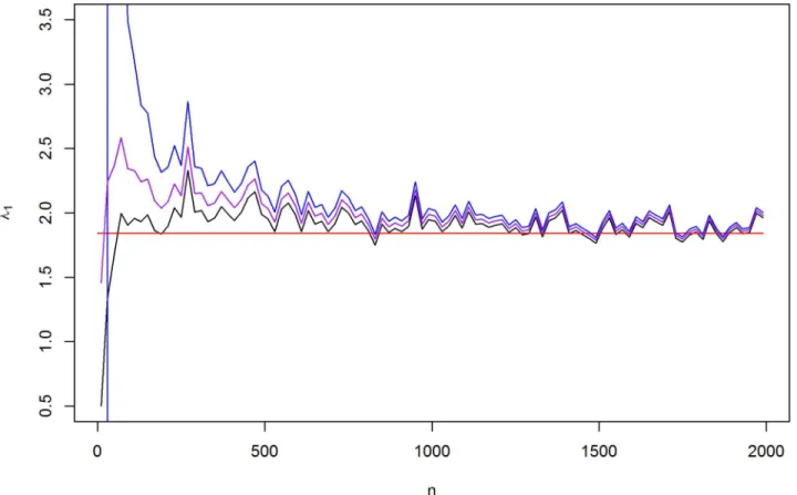
covariance matrix. The shrinkage functionF(l) approaches the MLE-based eigenvalue 1/l whenpisfixed andnincreases. This systematic shrinkage of the eigenvalue is illustrated inFig 1, where the red line indicates the largest eigenvalue of the realΘ. The ML-estimate tends to
amplify the largest eigenvalue even whennp. For eigenvalues of a covariance matrix with a different choice of the scale matrix, see [20].
Using the fact that the estimator for the covariance matrix is just the decomposition of the F(l) inverse with the same eigenvectors as the MLE, the linear type shrinkage of the eigenvalues of the covariance matrix isn
aliþ
a
a,i= 1,. . .,p. Instead of the eigenvalues of the precision
matrix, we take a look at the covariance matrix eigenvalues. This is because it is much easier to examine the linear shrinkage of the sample covariance matrix eigenvaluesli, which are always
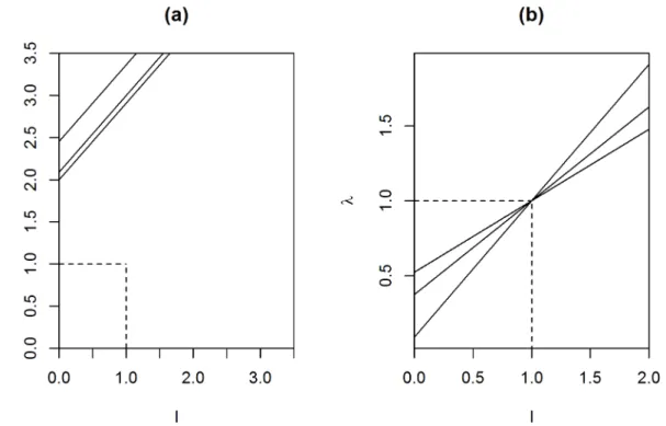
greater than or equal to zero, than the eigenvalues of the ML-based precision matrix estimate, which are not always determined. Whenn<p, the difficulty of selecting a proper scale param-eterαarises from the problem of choosing a value that shrinks large eigenvalues and increases the smaller ones to make the estimate positive definite. InFig 3ait can be seen that whenα
increases,αr, all sample eigenvalues grow whenn<pand the increment becomes greater, in accordance withα. In cases whenSis close to singularity this may lead to better results as small sample eigenvalues increase dramatically. Another possibility is to choose scale parame-terαasr−p−1 for the MAP ofSand thus forΘ. With this choice ofα, the Wishart prior increases sample eigenvalues lesser than one and shrinks eigenvalues greater than one. Also, the stable eigenvalues (li= 1) do not change. In this case, when the sample size increases the
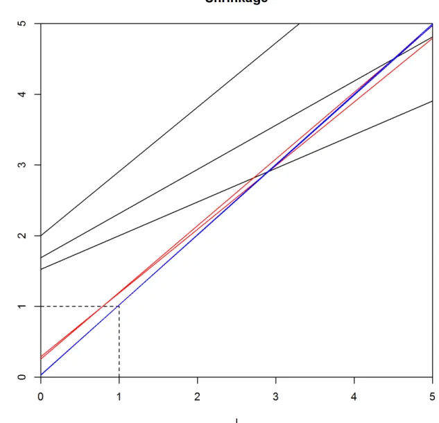
shrunken eigenvalues approach the sample eigenvalues, which is desirable whennp. This is presented inFig 3b, where the line denoting the shrinkage functionF(l)−1=λbecomes steeper whennincreases. We may posit that this feature makes it a safe choice whennp. However, the best choice could be a compromise between these two options for the relation ofrandα. Thus, one can choose hyperparametersrandαas equal. This case is illustrated inFig 4. Fig 1. The shrinkage of the largest eigenvalues.The largest eigenvalue of MAP (black line), ML-estimate (blue line), posterior mean (purple line) and the real eigenvalue ofΘ(red line) when the data is sampled from N(0,Θ−1) distribution with sample sizenandp= 20.
Choosing the degrees of freedom parameter
The choice of the degrees of freedom parameterrfor the Wishart priorW(r,α−1I) determines how much shrinkage is induced to the eigenvalues of a sample covariance matrixSwhen calcu-lating the MAP. In [5], it is proposed that the condition number of the covariance matrix esti-mate should be restricted by some values in order to gain a stable, well-conditioned estiesti-mate. The condition number of the MAP-estimate is defined ascond(ΘMAP) =λ1/λp, whereλ1is the
largest andλpthe smallest eigenvalue ofΘ
MAP. Clearly, the ratioλ1/λpis very large when the
MAP-estimate is close to singularity and, by increasing the small eigenvalues, may lead to bet-ter estimate. The value ofαis set asα=r. The condition number can be monitored andr
increased until thecond(ΘMAP) is smaller than a predetermined value. More informative prior
should be used whennpbecause the estimate is assumed to be sparse and the sample covari-ance matrix unreliable. In our numerical experiments, the restricted condition number was chosen to be smaller thancondðY
MAPÞ 2=
ffiffiffi
n p
, where the value of2=pffiffiffindiminishes as the
number of observations increases, leading back to use of non-informative Wishart prior. It should be noted that in high dimensional case, small eigenvalues of the sample covariance are very close to zero and posterior eigenvalues are approximatelyα/(n+r−p−1). Thus, it may Fig 2. Boxplots of the eigenvalues.From left to right: The eigenvalues of the real precision matrix, the maximum likelihood estimate (MLE), graphical lasso (Glasso,ρchosen with 5-fold cross-validation) and MAP of WishartW(2p, 1/2pI) prior when the true precision matrix is sparse (as described in section 3) with sample sizes of 30, 50, 100 and 1000.
be concluded that they are determined by the sample size and dimension, whenαandrare set as uninformative.
Decision-rule for sparse precision matrix estimation
With a ridge-type posterior estimate of the forma(nS+B−1)−1, it is impossible to set elements of estimated precision matrices exactly to zero, with any kind of choice in the degrees of free-dom parameter of the Wishart prior. This will always be a problem when using continuous prior distributions, because the resulting posterior probability of {θij} being zero is
non-exis-tent. Therefore, some external procedure should be used to set appropriate off-diagonal ele-ments exactly to zero. We propose a decision-rule process based on thresholding the smallest elements in the precision matrix in a stepwise manner using extended Bayesian information criterion (EBIC) to produce a sparse posterior estimate ofΘ.
Suppose we are interested in gaining a sparse posterior estimate forΘ. As mentioned by
[21], the Bayesian information criterion (BIC) tends to produce dense graphs in high dimen-sions. We have also faced similar problems in other simulation studies and in empirical data studies outside of this work. Thus we propose to use the EBIC instead of the BIC for the deci-sion-rule to choose the sparsity level of the estimatedΘ. This usually leads to more sparse
esti-mate for the precision matrix and thus sparser but still consistent graph topology for Gaussian graphical models. For more about EBIC, see [22].
The EBIC is of the form
EBIC¼ n½logðjYbjÞ trðYbSÞ þdfðYbÞlognþ4dfðYbÞglogp;
whereYb is the sparse posterior estimate ofΘanddfðYbÞis the number of non-zero elements Fig 3. Linear shrinkage of the eigenvalues.Shrinkage of the eigenvalues of the MAP of the covariance matrix, asris fixed andαchanges whenn<p(a) and withα=r−p−1 as the sample sizenincreases (b). The x-axis denotes the eigenvalues of the MLE (l) and y-axis denotes the corresponding
eigenvalues of the posterior estimate (λ=Φ(l)−1).
inYb, logðjYbjÞ trðYbSÞis the unnormalized log-likelihood andγis a user specified parame-ter which can be set as 0.5 as a default [22]. Here, the smaller value of EBIC indicates its better
fit for the model.
We use an universal thresholding method to induce sparsity to the Bayes estimate ofΘ. We
apply a stepwise selection and pick the posterior estimate with maximum level of sparseness, which minimizes the EBIC. The decision-rule works in the following manner.
LetA= (aij) be a symmetric matrix where elements are the absolute values of the posterior
estimate of the precision matrixΘ,a
ij¼ jbyijjfor alli,j= 1,. . .,p.
The non-zero elements ofYb are obtained by using the following algorithm:
Fig 4. Linear shrinkage of the eigenvalues.Shrinkage of the eigenvalues of the MAP of the covariance matrix asr=α. Whenn<p, all eigenvalues increase whenris small but whenrincreases, the increment gets more moderate (black lines). Whennincreases, shrunken eigenvalues get closer to the sample eigenvalues and the growth ofrdoes not significantly affect the estimated eigenvalues (red lines). Whennp, estimated eigenvalues start to coincide to the sample eigenvalues (blue lines).
1. Set thep(p−1)/2 off-diagonal elements ofAin ascending order as a vectora(1)a(2). . .
a(p(p−1)/2). 2. Initializel= 1.
3. Ifaija(l), setbyij¼byji¼0,i6¼jand setYbl¼ ðbyijÞfor alli= 1,. . .,p−1,j= (i+1),. . .,p,
i6¼j.
4. Calculate the EBIC for theYbl.
5. Setl=l+1.
6. Return to step 3, or stop if stopping criterion, e.g.l=p(p−1)/2 + 1, is met.
Select suchYb
kas the sparse posterior estimate ofΘwhich minimizes EBIC. We did not
apply any additional stopping criterion for the algorithm in our studies. For a largepthis is a greedy procedure but it can be executed in less thanp(p−1)/2 steps by using e.g. pre-defined threshold values or examining the monotonicity of the EBIC by plotting it against the number of non-zero elements of the sparse posterior estimate corresponding to the value of EBIC.
We are more interested in of these kind of methods, which are easy to run with minimal adjustment of any model value whatsoever. This approach is straightforward and has some similarities with the special thresholding, which can be applied to the entries of the sample covariance matrix in the graphical lasso algorithm [23], [11]. These expansions can be wrapped around the graphical lasso to gain a boost in the execution time. This resembles our method but with pre-defined threshold values.
With a moderate sample size covering a couple of hundred of variables, this is a feasible design and is invariant under permutation of variables. This procedure can be used in any Bayes estimate of the precision matrix. Without any mathematical justification we will show in numerical examples that this procedure works surprisingly well in both risk minimization set-tings and in data analysis and does not violate the positive definiteness restriction ofYb.
It should be noted that setting some elements to zero may lead to a non-positive definite posterior estimate ofΘ. In this case, a suitable valueδ>0 can be chosen to makeYb positive definite by adding it to the diagonal ofYb. Also, because the same threshold is used for all the precision matrix elements in our stepwise decision-rule procedure, the variables should be standardized to the same scale.
Simulation study
We were interested to see how the sample size affect the posterior estimate and the perfor-mance of our method when using the simple Wishart prior. To measure the perforperfor-mance of the analytic Bayesian procedure of usingW(r,α−1I)-prior together with the aforementioned decision-rule, 50 simulated data sets fromN(0,Θ−1) distribution were generated. Three unstructured and three structured matrices forΘandSwere considered in following fashion.
1. A diagonal matrix with elements randomly sampled from Uniform distribution;θkk* Uni-form(1, 1.25).
2. An autoregressive AR(1) matrix forS= (σ)kk0withσkk0= 0.7|k−k 0|
.
3. An AR(2) matrix withθkk= 1,θkk−1=θk−1k= 0.5 andθkk−2=θk−2k= 0.25. 4. A sparse matrix forΘwith at least 80% off-diagonal elements set to zero.
6. A dense matrix forΘwith less than 5% off-diagonal elements set to zero.
A Cholesky decomposition was used to generate the three unstructured positive definite matrices described in d), e) and f), following the approach of [4]. The dimensionpwas fixed to 20 andnwas chosen to be 10, 20, 50 and 100 for each of the 50 data sets.
Performance measures
Three different loss functions were used to compare the risks of the estimated precision matrix b
Y. The Kullback-Leibler loss (K-L) or the entropy loss, defined as
KLðY;YbÞ ¼trðY 1YbÞ logðjY 1YbjÞ p, theL2-loss (L2) defined asL2ðY;YbÞ ¼
jjY Ybjj
Fand the quadratic loss (Ql) defined asQðY;YbÞ ¼trðY
1 b
Y IÞ2. All measures approach zero as the estimateYb approaches the real precision matrix.
We used three other estimators for bothSandΘas baselines to compare the performance
of our decision-rule with prior having diminished condition number forΘ.
• Ledoit and Wolf estimator [19]. This is a frequentist estimator, or an empirical Bayes method where data driven parameters are used in the inverse Wishart prior assigned toS. This pro-duces a non-sparse shrinkage estimate forS. We invert this estimate to get the estimate ofΘ.
• Bouriga and Féron model 1 [20]. This is a hierarchical Bayes model forSwhere flat improper priors are assigned to both degrees of freedom and the scale matrix of the inverse Wishart distribution. This will lead to a ridge-type non-sparse posterior estimate forS. The estimator ofSwith respect to the squared Frobenius loss function (see [20]) was used in this simulation study. We calculated 10000 iterations with the Metropolis-within-Gibbs algorithm among which 5000 of the first MCMC samples were ignored as the burn-in period. Again the poste-rior estimate ofSis inverted to gain the estimate ofΘ.
• Graphical lasso (Glasso) is currenty considered as a state-of-art approach for sparse precision and covariance matrix estimation within the frequentist framework. Thus,“glasso”R pack-age [3] based on the algorithm 2 of [11] was used as a baseline to compare our results with each matrix and data combination. The regularization parameterρneeded in the Glasso algorithm was chosen by EBIC as described earlier. The candidate sequence forρwas chosen as [0.01, 0.02, 0.03,. . ., 0.5].
For both our method and Glasso the default value ofγ= 0.5 was used in this simulation study for the EBIC. All methods were run with R but the analysis concerning the Bouriga and Féron posterior estimate was performed with MATLAB.
For our estimator, the MAP was used as the point estimate of the precision matrix, because it induces more shrinkage to the eigenvalues than the posterior mean. The mean and standard deviation were calculated for each loss function, based on 50 different data replicates to com-pare these frequentist risk measures. See [24] for loss measures in MCMC sampling.
Results
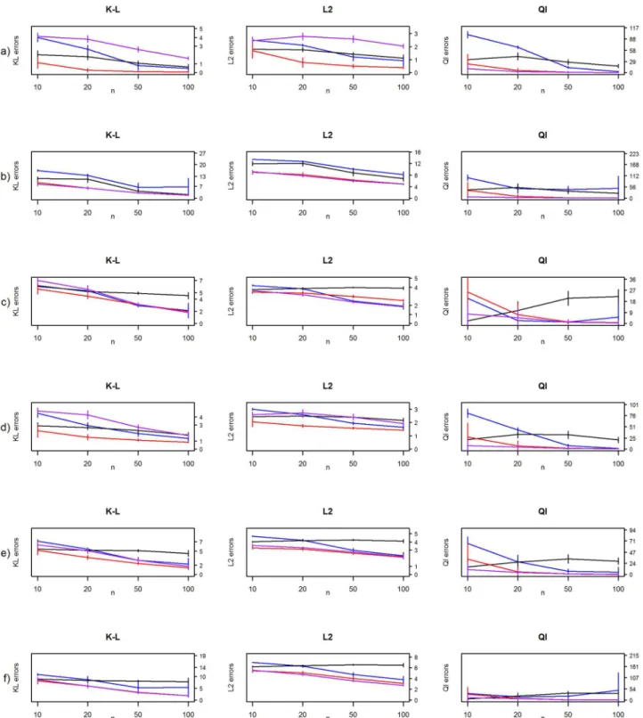
Fig 5. Frequentist risk estimates from the simulation studies.Kullback-Leibler (K-L), L2-loss (L2) and quadratic losses (Ql) for MAP-estimate with diminished condition number combined with decision-rule (blue line), hierarchical Bayes model by Bouriga and Féron (purple line), the Ledoit and Wolf estimate (red line) and graphical lasso algorithm (black line) for (a) diagonal, (b) AR(1), (c) AR(2), (d) sparse, (e) moderate and (f) dense precision matrices.
We are surprised by the moderate performance of the graphical lasso in this simulation set-ting. Even when the sample size increases, the risk measures do not diminish, and that is quite unexpected. This is most certainly due the EBIC used to choose the regularization parameterρ. Still this is out of tune with our method in which performance is more consistent with the sam-ple size. Both the MAP-estimate with diminished condition number combined with our deci-sion-rule and Glasso stumble with AR(1) and dense precision matrices. Furthermore, the true matrices of these models have the highest condition numbers, at 28.55 and 28.94 respectively.
The dark horse in this simulation study is the Ledoit and Wolf estimator which gives the smallest frequentist risk with all measures in almost all cases. It is also clearly the fastest method compared to the others. The Bouriga and Féron model provides competent estimates and particularly the lowest risk for the quadratic loss. The only problem with this approach is the time which is used in the Gibbs sampling even with our moderate MCMC sample size. This is the Achilles’heel of the hierarchical Bayesian models in the covariance and precision matrix estimation where the time and computing power needed for the analysis is a common problem. For example [9] reported a computation speed of about a minute for a block Gibbs sampler for
p= 100. Our method takes mere seconds to perform in the same dimension.
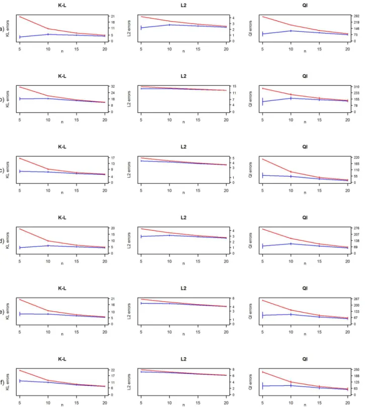
InFig 6, weakly-informative prior is compared to uninformative prior without decision-rule. The Wishart prior where the degrees of freedom parameter was set to be weakly-informa-tive outperforms the uninformaweakly-informa-tive Wishart prior in all cases whennp, and performs at a similar level when there are more data points. This is in line with the suggestions of [17]. Of particular note is the fact that the performance measures under quadratic loss decrease in every case. In our numerical studies, the decision-rule always produced a sparse and positive definite MAP-estimate forΘ, negating the need for an ad hoc correction to the eigenvalue structure of
the estimate. This included tens of thousands of sparse MAP-estimates.
Empirical Bayes method for sparse precision matrix estimation
There may be a special case when there is a reason to assume that just a few off-diagonal ele-ments of the precision matrix are non-zero, similar to the matrix d) described at the beginning of the section 3. The previous subsection indicated that the Ledoit and Wolf estimator is able to produce low risk estimates forΘin general.
The Ledoit and Wolf estimator is a ridge-type estimator of the formρ1I+ρ2Swhereρ1and
ρ2are specific parameters determined by the data (for more details, see [19]). It can be seen
that all the ridge-type estimators of the above-mentioned form have a Bayesian interpretation of the formS *W−1(n/ρ
2−n+p+ 1,nρ1/ρ2I) for the covariance matrix which will lead to
the ridge-type estimate for the posterior mean—or for the MAP in the similar matter. The prior for the precision matrix is the Wishart prior withρ2/nρ1Iset as the scale matrix. Thus,
we use the Ledoit and Wolf estimator as an empirical Bayes estimator forΘ. Our goal is to
improve the estimator of the precision matrix in the sparse setting by using our decision-rule procedure with the Ledoit and Wolf estimator. In this chapter we examine the performance of this approach whenp>nand refer to the Ledoit and Wolf estimator with our decision-rule procedure shortly as an empirical Bayes estimate.
Fig 6. Frequentist risk estimates from the simulation studies.Kullback-Leibler (K-L), L2-loss (L2) and quadratic losses (Ql) for (a) diagonal, (b) AR(1), (c) AR(2), (d) sparse, (e) moderate and (f) dense precision matrices for diminished condition number (blue line) and common Wishart prior based MAP (red line) withrandαset asp.
criterion for Glasso but this resulted in high frequentist risk estimates (results not shown) com-pared to the ones presented inTable 1.
The performance of the Glasso improves substantially when using the 5-fold cross-valida-tion. Now the Glasso is able to give comparable results and even outperform our empirical Bayes estimate. The Glasso seems to have some problems with consistency in this setting because the risk estimates appear not to decrease as the sample size increases. Still our empiri-cal Bayes method gives lower risk in some of the cases and seems to be consistent as the sample size increases. Again, the decision-rule always produced a positive definite estimate with no need to tamper with the final sparse estimate. Because the Ledoit and Wolf estimator does not need any iteration whatsoever, the empirical Bayes estimate can be calculated almost instantly and the stepwise decision takes about 20 seconds to be executed whenp= 100.
The choice between EBIC and cross-validation is a trade off between two features. Glasso with EBIC produces way more sparse structure for the estimate ofΘthan with the
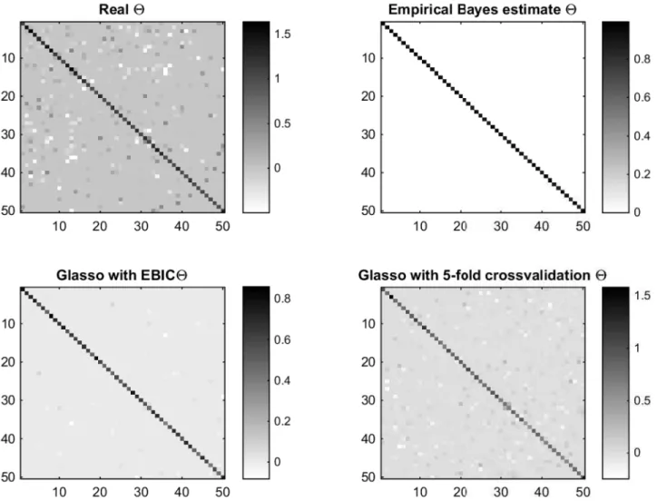
cross-valida-tion. As mentioned by [21], the cross-validation tends to produce dense graphs with many false positive edges. This is not desirable if the Glasso is used in the graph estimation in high dimensions. As illustrated inFig 7, the Glasso with 5-fold cross-validation seems to be closer to the real structure of theΘand the Glasso estimate with EBIC has just few non-zero
off-diago-nal elements. On the other hand, the empirical Bayes estimate produces way too sparse esti-mate with no sign of the structure of the true precision matrix with this data set. In the next section we will see that this“over-sparsity”is not a problem whennp.
Application to real data
In this chapter, we extend previously examined estimates for the precision matrix to the graph estimation in a real data example. First we introduce some concepts needed for the graph construction.
Denote thatG¼ ðN;EÞis a graphical model with node setN ¼ f1;. . .;pgand edge setE
inN N. One can parallel the nodes with the variables of interest. We estimate the graph
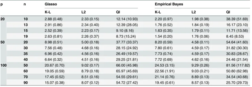
associated with the GGM by using the elements of the precision matrix to compose a Table 1. Simulation results for different precision matrices.
p n Glasso Empirical Bayes
K-L L2 Ql K-L L2 Ql
20 10 2.88 (0.48) 2.33 (0.15) 12.14 (10.93) 2.20 (0.97) 1.98 (0.38) 38.39 (51.69)
13 2.91 (0.86) 2.34 (0.40) 12.39 (28.05) 1.76 (0.52) 1.84 (0.19) 16.17 (23.10)
15 2.52 (0.39) 2.23 (0.17) 9.10 (8.16) 1.63 (0.35) 1.79 (0.11) 11.71 (13.56)
19 2.63 (0.81) 2.26 (0.37) 8.73 (15.24) 1.54 (0.20) 1.76 (0.06) 8.45 (8.53)
50 20 8.98 (0.51) 5.00 (0.18) 37.77 (33.37) 8.20 (0.59) 4.58 (0.11) 54.64 (41.60)
30 7.56 (0.48) 4.68 (0.16) 28.15 (24.92) 7.80 (0.61) 4.59 (0.17) 31.82 (30.30)
35 6.96 (0.42) 4.56 (0.16) 26.49 (19.57) 7.73 (0.74) 4.59 (0.17) 30.83 (28.67)
40 6.64 (0.32) 4.51 (0.16) 29.25 (21.81) 7.72 (0.69) 4.62 (0.16) 24.46 (21.54)
100 50 20.67 (0.70) 9.02 (0.17) 66.00 (45.98) 24.53 (3.15) 9.29 (0.26) 81.56 (117.82)
60 19.05 (0.59) 8.79 (0.18) 65.97 (45.69) 22.56 (1.91) 9.03 (0.21) 50.80 (62.98) 70 17.45 (0.52) 8.51 (0.16) 54.55 (29.61) 21.14 (0.76) 8.89 (0.13) 34.54 (40.68) 90 15.07 (0.38) 8.07 (0.12) 54.72 (27.42) 19.45 (0.61) 8.57 (0.13) 25.70 (29.73) Risk measures based on the frequentist means and standard deviations of Kullback-Leibler (K-L), L2 and quadratic (Ql) losses for graphical lasso (Glasso) and empirical Bayes (Ledoit and Wolf) estimator combined with our decision-rule.
symmetric adjacency matrix. IfYb is an estimate of the precision matrix, one can construct an adjacency matrixAd, (Adij)2{0, 1},i,j= 1,. . .,p, in the following manner.
Adij¼
1; if Y
ij6¼0:
0; otherwise: ð
5Þ
(
The pair (i,j) is contained in the edge setEif and only if the elementAdijis non-zero. The
diagonal of the adjacency matrix can be set as zero so that there are no pairs (i,i) in the edge set. To illustrate the estimated graphGb, we drew a edge between the nodes (variables) (i,j),i6¼ jif the elementAdijis one. Otherwise there is no edge between the nodes and we posit that the
variableiis conditionally independent of the variablejgiven all remaining variables (see for example [26]). For this reason, one only needs to examine either the upper or the lower diago-nal elements of the adjacency matrixAd.
For reasons of clarity, a flow cytometry dataset from [13] is analyzed. A data frame from R-package“gss”(https://cran.r-project.org/web/packages/gss/index.html) containing 7466 cells, Fig 7. Image plots of the precision matrices.From left to right at the first row: The image plot of the realΘand empirical Bayes estimate. On the second
row: Graphical lasso with the penalization parameterρchosen with EBIC and graphical lasso withρchosen with 5-fold cross-validation whenp= 50 and
n= 40.
with flow cytometry measurements of 11 phosphorylated proteins and phospholipids on the log10scale of the original, is used. The networks were inferred with our decision-rule applied to
various aforementioned Bayes estimates, Glasso and Meinshausen and Bühlmann approxima-tion (MB approximaapproxima-tion) [27] contained in the“glasso”package. The results were compared to the undirected graph presented in [4]. A directed acyclic graph of the data can be found in [3], and an undirected graph similar to ours from [4]. Unlike [4], we used standardized data and did not precorrect the systematic effects from the data. The precorrection could reduce some edges between the nodes in the network with graphical lasso.
We applied our decision-rule to three different Bayesian Wishart based methods; our MAP-estimate with diminished condition number, Ledoit and Wolf MAP-estimate and the posterior esti-mate defined according to the model 1 of Bouriga and Féron [20]. For the Metropolis-within-Gibbs estimation of Bouriga and Féron, we used 20000 MCMC iterations with 5000 as the burn-in period to determine the final posterior estimate using the MATLAB. Other analyses were done with R.
For Glasso, we used the EBIC to choose the penalization parameterρfrom the sequence [0.01, 0.02, 0.03,. . .0.8] in the hope of attaining sparse graph. We used this same value in the
MB approximation. The estimated graphs based on the precision matrix are shown inFig 8. We also investigated how the methods performed in the estimation of the graphical struc-ture compared to the network of Sachs. For this, we computed the specificity, sensitivity,
fall-Fig 8. Undirected graphs from cell-signaling data.The original undirected graph from [13] (Sachs) and GGMs estimated with MAP with diminished condition number and decision-rule (MAP), graphical lasso (Glasso), Meinshausen and Bühlmann approximation (MB approximation), Ledoit and Wolf estimate with our decision-rule (Ledoit & Wolf) and posterior forΘestimated with the model 1 introduced by Bouriga and Féron with our decision-rule
(Bouriga & Féron).
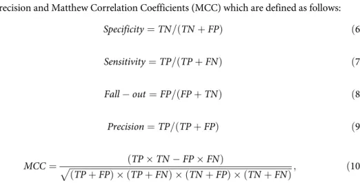
out, precision and Matthew Correlation Coefficients (MCC) which are defined as follows:
Specificity¼TN=ðTNþFPÞ ð6Þ
Sensitivity¼TP=ðTPþFNÞ ð7Þ
Fall out¼FP=ðFPþTNÞ ð8Þ
Precision¼TP=ðTPþFPÞ ð9Þ
MCC¼ ffiffiffiffiffiffiffiffiffiffiffiffiffiffiffiffiffiffiffiffiffiffiffiffiffiffiffiffiffiffiffiffiffiffiffiffiffiffiffiffiffiffiffiffiffiffiffiffiffiffiffiffiffiffiffiffiffiffiffiffiffiffiffiffiffiffiffiffiffiffiffiffiffiffiffiffiffiffiffiffiffiffiffiffiffiffiffiffiffiffiffiffiffiffiffiffiffiffiffiffiffiffiffiðTPTN FPFNÞ
ðTPþFPÞ ðTPþFNÞ ðTNþFPÞ ðTNþFNÞ
p ; ð10Þ
in whichTNis the number of true negatives,FPis the number of false positives,TPis the num-ber of true positives andFNis the number of false negatives. TheMCCcan vary between−1 and 1. The closer the values of specificity, sensitivity, precision and MCC are to one, the better the classification is. For the fall-out (aka the false positive rate), which is the same as 1− speci-ficity, the value closer to zero is better. The results are presented inTable 2.
Comparing graphs in theFig 8it appears that all of the Bayesian methods produce more sparse graphs than the Glasso and MB approximation. The diagnostics in theTable 2indicate that the Bayesian approaches performed at least comparable manner to the frequentist compet-itors. We note, that the MCC is higher with the frequentist methods. On the other hand, these methods produce the highest fall-out and sensitivity, which is due to the dense graph estimates. From the practical point of view, the Bayesian methods produce graphs which are visually eas-ier to examine. The MAP-estimate and the Bouriga and Féron estimate differ from each other by just one edge (the edge between variables‘Erk’and‘Raf’). Overall the MAP-estimate with our decision-rule is able to detect false positive edges from the graph associated with this data set quite efficiently.
We noticed that with the default choice of the EBIC parameterγ= 0.5, the networks are quite dense. When we increased theγover the value 0.6, it reduced the number of the estimated edges but beyond this point the increment of the parameter had no effect to the graph struc-ture. The graphs presented in theFig 8are derived from theγset as 0.6.
Glasso and MB approximation tend to favour dense graph structure and the adjustment of the parameterγhad whatsoever effect to the number of edges in the graph. This may be due to the weight of the likelihood which causes the Glasso to be close to the ML-estimate whenn
Table 2. Diagnostics for competing methods.
MAP Ledoit & Wolf Bouriga & Féron Glasso M & B approximation
Specificity 0.583 0.528 0.611 0.222 0.250
Sensitivity 0.632 0.632 0.632 1.000 0.947
Fall-out 0.417 0.472 0.389 0.778 0.750
Precision 0.444 0.414 0.462 0.404 0.400
MCC 0.204 0.152 0.231 0.300 0.243
Summary of specificity, sensitivity, fall-out, precision and Matthew Correlation Coefficients (MCC) for the MAP-estimate with regularized condition number (MAP), Ledoit and Wolf estimate, Bouriga and Féron posterior estimate, graphical lasso (Glasso) and Meinshausen and Bühlmann approximation when the estimated graphs are compared to the“Sachs”graph.
p. We also tried the analysis with the 5-fold cross-validation but the results were identical to those with regularization parameter chosen by EBIC.
The inferred networks drawn from the estimated precision matrices may be dense because there are several edges between nodes which are redundant, such as the node between PKC and Erk. From the original network of [13] we can see that both PKA and Erk are downstream of PKC and, thus, PKC is conditionally independent of Erk given PKA and other variables; that is, (PKC?Erk | other variables). Based on [13], there are also some unmeasured variables which cause indirect connections.
Discussion
We have proposed improvements to the classic Bayesian estimates when using Wishart prior for the precision matrix by just increasing the degrees of freedom parameter of the Wishart prior. By monitoring the condition number of the estimate, we can determine an estimate with lower risk, without loss of computational speed. Apart from graphical lasso, analytical preci-sion estimates for the matrix elements are available and can be calculated without iterative methods or MCMC sampling. Whenp/n1, Wishart prior, combined with a decision-rule step where few additional elements are set to zero, may be a good choice for sparse precision and covariance matrix estimation.
The simulations with several sparsity patterns of the precision matrix indicate that there is no happy compromise between sparse estimate for the precision matrix and low risk estimate when measured with the loss-functions we have used. In the regression-based lasso approach, we know that the cross-validation does produce a model with a reliable prediction ability but this generally does not lend itself to a very sparse model [28] without some pre-modification of the data [4].
From this, a contradiction arises in terms of classic Bayesian analysis. When there are more data points, it is natural that the data starts to dominate over the prior and the posterior esti-mate comes closer to the MLE. This is troublesome because it may cause overly dense graphs when the true precision or covariance matrix is sparse. However, as can be seen from our example with the flow cytometry data, whennp, our decision-rule is able to produce a sparse graph whereas graphical lasso is able to produce only moderately sparse graph. Artificial adjustment of the penalization parameterρof the graphical lasso will produce a sparser net-work (cf. [8], [3], [4], [9]) but we wanted to avoid this kind of unjustified analysis. Also meth-ods such as stability approach to regularization selection (StARS) [21] could be used with the graphical lasso. We tested this with the R package“huge”[29]. With StARS, the Glasso derived network was very sparse (just eight edges) with the following diagnostics: Specificity 0.944, sen-sitivity 0.316 fall-out 0.056, precision 0.750 and MCC 0.351. Clearly the performance of the Glasso depends on the procedure used to choose the regularization parameter.
It is possible to simulate independent posterior samples and obtain credible regions for the whole precision matrix because of the known analytic posterior distribution. In [4], credible region based thresholding is used to choose which off-diagonal elements should be set at zero; if the credible region contained a value of zero, the corresponding off-diagonal element was set as zero. We also tried this kind of strategy but found it to be inferior to EBIC-strategy with respect to both time and performance. Furthermore, this approach has the problem of choos-ing the width of the (1−α)100% credible region. In our simulation study the 95% credible region was not an efficient way to set putative off-diagonal values to zero. They also used arbi-trary 30% credible intervals in [4], which we found to be unsatisfactory in our own experi-ments. Additionally, in our Wishart setting the credible region-based approach does not guarantee that the sparse posterior estimate ofΘwould be positive definite and, thus, some ad
With documented experiments, a variety of different estimation approaches (including our approach) support the fact that there still does not exist an all-purpose procedure for covari-ance and precision matrix estimation in all problem settings. The real structure of the precision matrix and the choice of loss function significantly affect the final result, as noted by [20]. What makes stepwise thresholding a viable alternative is that it can be very fast in special cases, has no convergence problems typical for MCMC sampling, can work at a similar level to graph-ical lasso—or even better whenp/n1—and appears to be consistent when using the EBIC.
Supporting Information
S1 Code Collection. Collection of R codes used in this article.
(7Z)
Acknowledgments
We are grateful to our editor, two anonymous referees and Ashley Last for their valuable com-ments, which helped us to substantially improve this manuscript. We also thank Olivier Féron for providing us the MATLAB code for the Metropolis-Within-Gibbs sampler presented in [20]. This work was supported by Biocenter Oulu.
Author Contributions
Conceived and designed the experiments: MK MJS. Performed the experiments: MK. Analyzed the data: MK MJS. Contributed reagents/materials/analysis tools: MK MJS. Wrote the paper: MK MJS.
References
1. Pourahmadi M. High-Dimensional Covariance Estimation. John Wiley & Sons: New York; 2013. 2. Pourahmadi M. Covariance estimation: the GLM and regularization perspective. Statistical Science.
2011; 26(3): 369–387. doi:10.1214/11-STS358
3. Friedman J, Hastie T, Tibshirani R. Sparse inverse covariance estimation with the graphical lasso. Bio-statistics. 2008; 9(3):432–441. doi:10.1093/biostatistics/kxm045PMID:18079126
4. Khondker ZS, Zhu H, Chu H, Lin W, Ibrahim JG. The Bayesian covariance lasso. Statistics and Its inter-face. 2013; 6:243–259. doi:10.4310/SII.2013.v6.n2.a8PMID:24551316
5. Won J-H, Lim J, Kim S-J, Rajaratnam B. Maximum likelihood covariance estimation with the condition number constraint. Technical report, Stanford University, Department of Statistics. 2009.
6. Huang A, Wand MP. Simple marginally noninformative prior distributions for covariance matrices. Bayesian Analysis. 2013; 8(2):439–452. doi:10.1214/13-BA815
7. Kubokawa T, Srivastava MS. Estimation of the precision matrix of a singular Wishart distribution and its application in high-dimensional data. Journal of Multivariate Analysis. 2008; 99(9):1906–1928. doi:10. 1016/j.jmva.2008.01.016
8. Bien J, Tibshirani RJ. Sparse estimation of a covariance matrix. Biometrika. 2011; 98(4):807–820. doi: 10.1093/biomet/asr054
9. Wang H. Bayesian graphical lasso models and efficient posterior computation. Bayesian Analysis. 2012; 7(4):867–886. doi:10.1214/12-BA729
10. Yuan T, Wang J. A coordinate descent algorithm for sparse positive definite matrix estimation. Statisti-cal Analysis and Data Mining. 2013; 6(5):431–442.
11. Witten DM, Friedman JH, Simon N. New insights and faster computations for the graphical lasso. Jour-nal of ComputatioJour-nal and Graphical Statistics. 2011; 20(4):892–900. doi:10.1198/jcgs.2011.11051a 12. Tibshirani R. Regression shrinkage and selection via the lasso. Journal of the Royal Statistical Society
Series B. 1996; 58(1):267–288.
14. Dempster AP. Covariance selection. Biometrics. 1972; 28:157–175. doi:10.2307/2528966
15. Rowe D. Multivariate Bayesian Statistics: Models for Source Separation and Signal Unmixing. Chap-man & Hall/CRC: Boca Raton; 2003.
16. Hsu C-W, Sinay MS, Hsu JSJ. Bayesian estimation of a covariance matrix with flexible prior specifica-tion. Annals of the Institute of Statistical Mathematics. 2012; 64:319–342. doi: 10.1007/s10463-010-0314-5
17. Gelman A. Prior distributions for variance parameters in hierarchical models. Bayesian Analysis. 2006; 1(3):515–533.
18. Leonard T, Hsu JSJ. Bayesian inference for a covariance matrix. The Annals of Statistics. 1992; 20 (4):1669–1696. doi:10.1214/aos/1176348885
19. Ledoit O, Wolf M. A well-conditioned estimator for large-dimensional covariance matrices. Journal of Multivariate Analysis. 2004; 88:365–411. doi:10.1016/S0047-259X(03)00096-4
20. Bouriga M, Féron O. Estimation of covariance matrices based on hierarchical inverse-Wishart priors. Journal of Statistical Planning and Inference. 2013; 143(4):795–808. doi:10.1016/j.jspi.2012.09.006 21. Liu H, Roeder K, Wasserman L. Stability approach to regularization selection (StARS) for high
dimen-sional graphical models. Advances in Neural Information Processing Systems. 2010; 23:1432–1440. 22. Foygel R, Drton M. Extended Bayesian information criteria for Gaussian graphical models. Advances in
Neural Information Processing Systems. 2010; 23:604–612.
23. Mazumder R, Hastie T. Exact covariance thresholding into connected components for large-scale graphical lasso. Journal of Machine Learning Research. 2012; 13: 723–736.
24. Yang R, Berger JO. Estimation of a covariance matrix using the reference prior. The Annals of Statis-tics. 1994; 22(3):1195–1211. doi:10.1214/aos/1176325625
25. Leßmann K. Probabilistic exposure assessment parameter uncertainties and their effects on model out-put. PhD-Thesis. University of Osnabrück. 2002.
26. Edwards D. Introduction to Graphical Modelling ( 2nd ed). Springer: New York; 2000.
27. Meinshausen N, Bühlmann P. High dimensional graphs and variable selection with the lasso. The Annals of Statistics. 2006; 34(3):1436–1462. doi:10.1214/009053606000000281
28. Li Z, Sillanpää MJ. Overview of lasso-related penalized regression methods for quantitative trait map-ping and genomic selection. Theoretical and Applied Genetics. 2012; 125(3):419–435. doi:10.1007/ s00122-012-1892-9PMID:22622521

![Fig 8. Undirected graphs from cell-signaling data. The original undirected graph from [13] (Sachs) and GGMs estimated with MAP with diminished condition number and decision-rule (MAP), graphical lasso (Glasso), Meinshausen and Bühlmann approximation (MB ap](https://thumb-eu.123doks.com/thumbv2/123dok_br/16469484.198954/16.918.63.653.534.970/undirected-signaling-undirected-diminished-condition-meinshausen-bühlmann-approximation.webp)