Submitted22 July 2015
Accepted 11 January 2016
Published28 January 2016
Corresponding author
Pawel Wasowicz, [email protected]
Academic editor
Jeffrey Ross-Ibarra
Additional Information and Declarations can be found on page 23
DOI10.7717/peerj.1645
Copyright
2016 Wasowicz et al.
Distributed under
Creative Commons CC-BY 4.0
OPEN ACCESS
Phylogeography of
Arabidopsis halleri
(Brassicaceae) in mountain regions of
Central Europe inferred from cpDNA
variation and ecological niche modelling
Pawel Wasowicz1,2, Maxime Pauwels3, Andrzej Pasierbinski2, Ewa M. Przedpelska-Wasowicz4, Alicja A. Babst-Kostecka5, Pierre Saumitou-Laprade6and Adam Rostanski2
1Icelandic Institute of Natural History, Iceland
2Faculty of Biology and Environmental Protection, Department of Botany and Nature Protection,
University of Silesia, Katowice, Poland
3Unité Evo-Eco-Paléo (EEP)—UMR 8198, Université de Lille—Sciences et Technologies, CNRS,
Villeneuve d’Ascq, France
4Institute of Botany, University of Warsaw, Warszawa, Poland
5Department of Ecology, Institute of Botany, Polish Academy of Sciences, Krakow, Poland 6Unité Evo-Eco-Paléo (EEP)—UMR 8198, Université des Sciences et Technologies de Lille (Lille I),
Villeneuve d’Ascq, France
ABSTRACT
The present study aimed to investigate phylogeographical patterns present within
A. halleriin Central Europe. 1,281 accessions sampled from 52 populations within the investigated area were used in the study of genetic variation based on chloroplast DNA. Over 500 high-quality species occurrence records were used in ecological niche modelling experiments. We evidenced the presence of a clear phylogeographic structure withinA. halleriin Central Europe. Our results showed that two genetically different groups of populations are present in western and eastern part of the
Carpathians. The hypothesis of the existence of a glacial refugium in the Western Carpathians adn the Bohemian Forest cannot be rejected from our data. It seems, however, that the evidence collected during the present study is not conclusive. The area of Sudetes was colonised after LGM probably by migrants from the Bohemian Forest.
SubjectsBiodiversity, Biogeography, Plant Science
Keywords Arabidopsis halleri, Harz, Quaternary, Carpathians, Taxonomy, Phylogeography, Sudetes, Alps
INTRODUCTION
contemporary populations (Médail & Diadema, 2009). The presence of this differentiation has allowed (with the advent of phylogeography) insights into processes responsible for range formation, reconstruction of (re)colonisation routes, detection of refugial areas and unravelling historical relationships among different parts of the contemporary species distribution.
Areas of relative ecological stability that provided suitable habitats for species survival during periods of glaciation are termed refugia (Tribsch & Schönswetter, 2003). Numerous studies carried out so far showed that major glacial refugia were located in the southern part of Europe (Taberlet et al., 1998; Hewitt, 1999). Recently, the possibility of full-glacial survival of temperate species at northern latitudes in so-called northern or cryptic refugia (Stewart & Lister, 2001) was hypothesised and subsequently supported by fossil records from several species (Willis & Van Andel, 2004). There is, however, still little molecular evidence for the existence of ‘‘northern refugia’’ in Central Europe (Daneck et al., 2011).
In Europe the potential for phylogeographical research has been exploited intensively in the Alps, where the abundance and complexity of the available phylogeographic studies has already resulted in synthetic and comparative analyses (Schönswetter et al., 2005;Alvarez et al., 2009). The situation is quite different in other mountain ranges of Central Europe such as the Carpathians, Sudetes, Bohemian Forest (Sumava) and Harz Mts. A recent literature review pointed out clearly that the history of species range formation in the mountains of Central Europe is still only poorly known from phylogeographical studies (Ronikier, 2011).
Arabidopsis halleriwith its pattern of occurrence covering nearly all mountain regions of Central Europe (Jalas & Suominen, 1994) seems to be an interesting model taxon to address all the problems raised above. Previous phylogeographical studies focused on the species, evidenced the presence of two major units within the species range and attributed the emergence of these units to vicariance associated with the isolation of two large populations groups during the Quaternary, which were located in Central and Southern Europe (Pauwels et al., 2012). The sampling density adopted in the study was, however, too low to address the question ofA. hallerirange formation in the mountains of Central Europe.
In the light of these considerations, we focused our study on the poorly investigated area covering the Carpathians, Sudetes, Bohemian Forest and Harz Mountains in order to reconstruct the phylogeographic history of this montane species Arabidopsis halleri. This approach allowed us to overcome another limitation originating from the fact that the vast majority of phylogeographical analyses carried out hitherto on mountain species in Europe has been focused on alpine and arctic-alpine species, while our knowledge of the phylogeographic patterns present within herbaceous species having the centre of its occurrence in lower vegetation belts (subalpine and montane) remains, with some notable exceptions (Despres, Loriot & Gaudeul, 2002;Stachurska-Swakoń, Cieślak & Ronikier, 2013), much poorer.
We aimed to answer the following questions:
1. Is there any geographically structured genetic variation in A. halleri within the investigated area?
2. Is there any evidence for the existence of glacial refugia in Central Europe? 3. What is the origin ofA. halleripopulations in the Carpathians and Sudetes?
MATERIALS & METHODS
The study speciesArabidopsis halleri(L.) O’Kane & Al-Shehbaz is a perennial, self-incompatible and highly outcrossing (Llaurens et al., 2008), stoloniferous herb with a highly disjunctive distribution between Europe and the Far East. It occurs in mountain and upland environments on slopes, forest margins, rocky crevices and river banks from 200 to 2,200 m a.s.l. In Europe, it is widely distributed in the Alps, Carpathians, Sudetes and Dinaric Alps (Jalas & Suominen, 1994). Its distribution also covers some upland regions north from the Alps (including the Harz Mountains) and the Western Carpathians (Jalas & Suominen, 1994). The species is highly variable in leaf morphology, flower colour and traits connected with the development of stolons. At least three subspecies are quite distinct in terms of morphological variation (Al-Shehbaz & O’Kane, 2002):A. hallerisubsp. halleriandA. hallerisubsp. ovirensisoccur in Europe, whereas A. hallerisubsp. gemmiferaoccurs in the Far East. According to other authors (Kolník & Marhold, 2006) the species can be alternatively divided into five distinct morphological subspecies, with four occurring in Europe. Only diploid (2n = 2X = 16) individuals have so far been reported from throughout the distribution range (Al-Shehbaz & O’Kane, 2002;Kolník & Marhold, 2006).
Other species from the genus Arabidopsis also co-occur within the investigated area
(A.thaliana,A.arenosa,A.neglecta,A. lyrata). A recent study has shown that reticulation and hybridization among lineages that might have transferred cpDNA types from one lineage into the other is unlikely (Koch & Matschinger, 2007). The same authors have pointed out that cpDNA type diversity may predate separation of the main evolutionary lineages within the genus (Koch & Matschinger, 2007).
Sampling and DNA extraction
We sampled 1,281 individuals from 52 populations (Table 1) scattered across the species
range in seven geographic regions of Central and Eastern Europe (seeFig. S1).
Table 1 Location of sampled populations and sample sizes.
GPS coordinates Altitude
Population Locality; collectors Latitude Longitude (m a.s.l.) n
A05 Mutters, Alps, Northern Tyrol, Austria; MP, PSL 47◦13′46.68′′ 11◦22′46.72′′ 807 14 A08 W from Mehrn, Alps, Northern Tyrol, Austria; MP, PSL 47◦25′10
.56′′ 11◦51′57.46′′ 522 45
A09 W from Mehrn, Alps, Northern Tyrol, Austria; MP, PSL 47◦25′14
.57′′ 11◦51′53.71′′ 519 20
CZ04 SW from Vimperk, Bohemian Forest, Czech Rep.; MP, PSL 49◦02′08.72′′ 13◦45′08.41′′ 772 14 CZ05 N from Kubova Hut’, Bohemian Forest, Czech Rep.; MP, PSL 48◦59′15
.54′′ 13◦46′23.40′′ 998 24
CZ06 Kubova Hut’, Bohemian Forest, Czech Rep.; MP, PSL 48◦59′00
.00′′ 13◦46′00.00′′ 1,060 12
CZ14 near Starý Herštajn, Bohemian Forest, Czech Rep.; MP, PSL 49◦28′37
.19′′ 12◦42′92.15′′ 842 20
CZ16 Horská Kvilda, Bohemian Forest, Czech Rep.; MP, PSL 49◦03′21
.05′′ 13◦33′18.19′′ 1,052 57
CZ18 NW from Zhuři, Bohemian Forest, Czech Rep.; MP, PSL 49◦05′42
.14′′ 13◦32′10.31′′ 1,039 9
CZ20 Labská, Sudetes, Czech Rep.; PW, EPW 50◦42′55
.9′′ 15◦35′00.9′′ 698 33
CZ21 Herlikovice, Sudetes, Czech Rep.; PW, EPW 50◦39′41
.6′′ 15◦35′44.5′′ 555 30
CZ22 Rýchorská Bouda, Sudetes, Czech Rep.; PW, EPW 50◦39′29
.4′′ 15◦51′00,00′′ 995 32
D01 NE from Ramspau, Bohemian Forest, Germany; MP, PSL 49◦10′06
.40′′ 12◦09′08.80′′ 345 7
D02 near Hirschling, Bohemian Forest, Germany; MP, PSL 49◦11′31
.00′′ 12◦09′52.00′′ 452 8
D03 W from Cham, Bohemian Forest, Germany; MP, PSL 49◦13′10
.00′′ 12◦39′66.00′′ 362 9
D04 S from Hochfeld, Bohemian Forest, Germany; MP, PSL 49◦09′50
.95′′ 12◦47′45.43′′ 383 11
D08 S from Oker, Harz Mts., Germany; MP, PSL 51◦53′47
.45′′ 10◦29′23.97′′ 279 12
D09 S from Glosar, Harz Mts., Germany; MP, PSL 51◦53′27
.55′′ 10◦25′05.62′′ 325 18
D11 E from Hahnemklee, Harz Mts., Germany; MP, PSL 51◦51′16
.17′′ 10◦21′56.68′′ 644 18
D12 SE from Lautenthal, Harz Mts., Germany; MP, PSL 51◦51′54
.09′′ 10◦17′53.85′′ 415 18
D13 SW from Langelsheim, Harz Mts., Germany; MP, PSL 51◦55′13
.40′′ 10◦18′29.68′′ 231 20
D14 SE from Heersum, Harz Mts., Germany; MP, PSL 52◦06′08
.66′′ 10◦06′57.62′′ 89 11
PL02 Żyglinek, Western Carpathian Foreland, Poland; MP, PSL 50◦29′40
.81′′ 18◦56′40.29′′ 298 21
PL03 W from Żyglinek, Western Carpathian Foreland, Poland; MP, PSL 50◦29′30
.34′′ 18◦57′34.57′′ 302 15
PL07 Ujków Stary, Western Carpathian Foreland, MP, PSL 50◦17′00
.92′′ 19◦29′03.10′′ 325 19
PL08 N from Chobot, Western Carpathian Foreland, Poland; MP, PSL 50◦05′51
.87′′ 20◦22′32.89′′ 193 12
PL32 Kościelisko, Western Carpathians, Poland; AK 49◦16′27
.72′′ 19◦52′45.58′′ 990 27
PL33 Zakopane, Western Carpathians, Poland; AK 49◦17′34
.02′′ 19◦55′34.59′′ 879 21
PL37 Szklarska Poręba, Sudetes, Poland; PW, EPW 50◦49′08.50′′ 15◦31′24.08′′ 690 40 PL38 Orle, Sudetes, Poland; PW, EPW 50◦49′00
.59′′ 15◦22′51.85′′ 828 29
PL39 E from Kowary, Sudetes, Poland; PW, EPW 50◦47′23
.66′′ 15◦51′55.82′′ 583 39
PL40 Kowarska Pass, Sudetes, Poland; PW, EPW 50◦45′37.77′′ 15◦52′04.37′′ 729 39 PL41 Hala Izerska, Sudetes, Poland; PW, EPW 50◦50′52
.36′′ 15◦21′45.62′′ 837 39
PL42 Łabski Szczyt, Sudetes, Poland; PW, EPW 50◦47′14
.47′′ 15◦32′17.18′′ 1,189 39
PL43 Mały Staw, Sudetes, Poland; PW, EPW 50◦44′54.90′′ 15◦42′09.56′′ 1,199 39 PL44 W from Zieleniec, Sudetes, Poland; PW, EPW 50◦22′54
.28′′ 16◦21′47.26′′ 755 41
PL45 Zawadzkie, Western Carpathian Foreland, Poland; PW, EPW 50◦37′23
.06′′ 18◦26′39.06′′ 208 39
PL46 Sianki, Eastern Carpathians, Poland; PW, EPW 49◦01′14.40′′ 22◦53′08.40′′ 800 23 PL47 Roztoki Górne, Eastern Carpathians, Poland; PW, EPW 49◦09′04
.30′′ 22◦19′16.90′′ 728 24
PL48 Krzywe, Eastern Carpathians, Poland; PW, EPW 49◦11′64
.00′′ 22◦21′28.80′′ 647 20
(continued on next page)
Table 1(continued)
GPS coordinates Altitude
Population Locality; collectors Latitude Longitude (m a.s.l.) n
PL49 Nasiczne, Eastern Carpathians, Poland; PW, EPW 49◦10′22
.90′′ 22◦35′50.80′′ 643 22
PL50 Łężyce, Sudetes, Poland; PW, EPW 50◦26′44
.8′′ 16◦20′58.3′′ 712 34
SK02 Vysný Klátov, Western Carpathians, Slovakia; MP, PSL 48◦46′10
.33′′ 21◦07′48.49′′ 586 22
SK05 NE from Javorina, Western Carpathians, Slovakia; MP, PSL 49◦16′59.11′′ 20◦09′14.51′′ 994 46 SK10 Štrbskié Pleso, Western Carpathians, Slovakia; PW, EPW 49◦07′07
.26′′ 20◦03′42.24′′ 1,322 21
SK12 Plihov, Western Carpathians, Slovakia; PW, EPW 49◦24′15
.30′′ 20◦42′08.52′′ 466 16
UA01 Rakhiv, Eastern Carpathians, Ukraine; PW, AR, PSL 48◦01′31.60′′ 24◦10′02.80′′ 434 31 UA02 Kvasy, Eastern Carpathians, Ukraine; PW, AR, PSL 48◦07′59
.00′′ 24◦16′26.10′′ 530 32
UA04 Vil’shany, Eastern Carpathians, Ukraine; PW, AR, PSL 48◦19′57
.60′′ 23◦36′22.80′′ 555 32
UA05 Synevyr, Eastern Carpathians, Ukraine; PW, AR, PSL 48◦32′04.80′′ 23◦38′53.50′′ 699 32 UA06 Synevyr Lake, Eastern Carpathians, Ukraine; PW, AR, PSL 48◦37′01
.20′′ 23◦41′10.20′′ 1,006 16
UA07 Synevyrska Poliana, Eastern Carpathians, Ukraine; PW, AR, PSL 48◦36′00
.60′′ 23◦41′54.30′′ 829 8
Notes.
n, sample size.
Collected leaf tissue was immediately dried in silica gel prior to molecular analysis.
DNA was extracted from 10 to 15 mg of dry material using NucleoSpinR 96 Plant
(Macherey-Nagel), and PCR amplifications were performed on 1:20 dilutions.
Genetic analysis Genotyping procedure
During the genotyping process we screened 12 polymorphic sites previously detected by PCR-RFLP in three cpDNA regions:trnK intron and two intergenic regions (trnC-trnD,
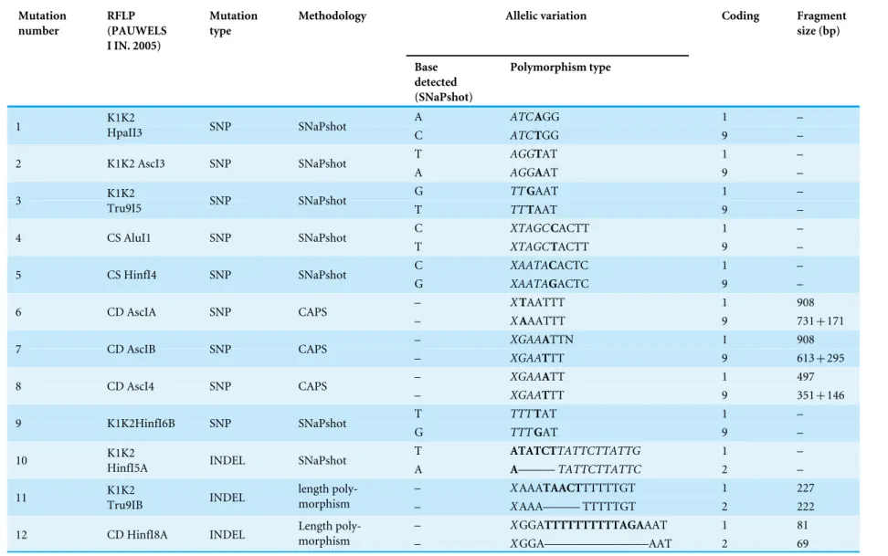
psbC-trnS). The observed polymorphisms are briefly characterized inTable 2. In contrast toPauwels et al. (2005), however, three different genotyping methods were employed.
SNaPshot assay
After PCR amplification of the three cpDNA regions of interest, we used SNaPshot assay for simultaneous detection of seven single nucleotide polymorphisms (SNP, cf.Table 2).
In the analysis we employed ABI PrismR SNaPshotR Multiplex Kit (Applied Biosystems)
and followed the protocol given by the manufacturer.
The following PCR conditions were utilized: a total volume of 15µl consisting of 3µl of template DNA (20–100 ng), 6.225µl of water, 1.5µl of 10X PCR Buffer, 2.1µl of 25 mM solution of MgCl2, 1.2µl of 2.5 mM solution of dNTP, 0.3µl of BSA solution (10 mg/ml),
0.3µl of 10 mM solution of each primer and 0.075µl of AmpliTaqRDNA Polymerase
(5U/µl). The reaction was carried out in MastercyclerR ep gradient S thermal cycler using one cycle of 5 min at 95 ◦C, and 36 cycles of 45 s at 92 ◦C, 45 s at 58 ◦C–62 ◦C (depending
of the primers sequences, precise protocol upon request); and 2 min 30 s at 72 ◦C, followed
by one cycle of 10 min at 72 ◦C. The primer sequences for specific PCR amplifications
are given inTable S1. Amplicons were used for genotyping ollowing the manufacturer’s
instruction (ABI PrismR SNaPshotR Multiplex Kit). The primer sequences used in the
Table 2 cpDNA polymorphism observed in investigated material.Observed mutations were numbered from 1 to 12 (numbers correspond with those given inFig. 1 and inTable 3).
Mutation number
RFLP (PAUWELS I IN. 2005)
Mutation type
Methodology Allelic variation Coding Fragment
size (bp)
Base detected (SNaPshot)
Polymorphism type
A ATCAGG 1 –
1 K1K2HpaII3 SNP SNaPshot
C ATCTGG 9 –
T AGGTAT 1 –
2 K1K2 AscI3 SNP SNaPshot
A AGGAAT 9 –
G TTGAAT 1 –
3 K1K2Tru9I5 SNP SNaPshot
T TTTAAT 9 –
C XTAGCCACTT 1 –
4 CS AluI1 SNP SNaPshot
T XTAGCTACTT 9 –
C XAATACACTC 1 –
5 CS HinfI4 SNP SNaPshot
G XAATAGACTC 9 –
– XTAATTT 1 908
6 CD AscIA SNP CAPS
– XAAATTT 9 731+171
– XGAAATTN 1 908
7 CD AscIB SNP CAPS
– XGAATTT 9 613+295
– XGAAATT 1 497
8 CD AscI4 SNP CAPS
– XGAATTT 9 351+146
T TTTTAT 1 –
9 K1K2HinfI6B SNP SNaPshot
G TTTGAT 9 –
T ATATCTTATTCTTATTG 1 –
10 K1K2HinfI5A INDEL SNaPshot
A A———TATTCTTATTC 2 –
– XAAATAACTTTTTTGT 1 227
11 K1K2Tru9IB INDEL length poly-morphism
– XAAA——— TTTTTGT 2 222
– XGGATTTTTTTTTTAGAAAT 1 81
12 CD HinfI8A INDEL Length poly-morphism
– XGGA————————–AAT 2 69
ABI PRISMR 3,130 xl Genetic Analyzer (Applied Biosystems) using a capillary of 36 cm,
POP 4 Migration Buffer and Dye Set E5. The data were collected using Foundation Data Collection 4.0 software and analyzed with GeneMapper 4.0.
CAPS assay
The CAPS assay was used for genotyping three SNP polymorphisms in thetrnC-trnD
region by specifically amplifying the genomic region containing the SNP polymorphisms mentioned inTable 2and digesting the amplification product using theAcsI restriction
enzyme. The PCR primer sequences were given in Table S2. The PCR mixture and the
conditions followed the protocol given above for SNaPshot assay. Restriction enzyme reaction was performed on a total volume of 20µl consisting of 10µl of PCR product and 10µl of restriction mixture containing 5.9µl of water, 2µl of SuRe/Cut Buffer B 10X, 2µl
of 2 mM solution of spermidine and 0.1 µl of AcsI solution (10U/µl). The mixture was
then incubated at 50 ◦C for 1 h, followed by enzyme deactivation at 70 ◦C for 15 min. Both
procedures were carried out in MastercyclerR ep gradient S (Eppendorf) thermal cyclers.
Fragments were separated by electrophoresis on 2% agarose gels stained by ethidium bromide and photographed with BioImage system (Bioprobe) under UV light.
PCR length difference assay
Two indel polymorphisms in thetrnK andtrnC-trnD regions (cf.Table 2) were genotyped
from a PCR product length difference assay following the method described byOetting et
al. (1995). The PCR mixture followed the protocol given above for SNaPshot assay. The primer sequences used in this reaction are given inTable S1. PCRs were carried out in MastercyclerR ep gradient S (Eppendorf) thermal cyclers using one cycle of 5 min at 95 ◦C, and 36 cycles of 30 s at 94 ◦C, 30 s at 51 ◦C or 56 ◦C (depending of the primers
sequences); and 30 s at 72 ◦C, followed by one cycle of 10 min at 72 ◦C. Fragments were
separated on 8% polyacrylamide gels using a Li-Cor 4200 Global IR2 DNA Sequencer.
Data analysis
Since cpDNA is a non-recombining molecule, alleles observed at all twelve loci were
combined into cpDNA haplotypes (chlorotypes,Table 3). Chlorotype nomenclature is
fully consistent with our previous study (Pauwels et al., 2005).
Phylogenetic relationships between chlorotypes
A minimum spanning tree (MST) was constructed on the basis of a distance matrix reflecting molecular differences between each pair of chlorotypes using a modification of the
algorithm described byRohlf (1973). Computations were made using the software Arlequin
Table 3 Description of cpDNA chlorotypes identified in investigated populations ofA. halleri.Characters used in coding correspond to coding column inTable 2. Correspondence to the mutations observed byPauwels et al. (2005)in RFLP study was given. Mutation numbers corresponds withFig. 1.
Mutation number
1 2 3 4 5 6 7 8 9 10 11 12
Mutation name (cf.Pauwels et al., 2005)
K1K1HpaII 3
K1K2 AcsI3
K1K1 Tru9I5
CS Alu I1
CS HinfI4
CD, AcsI 1A
CD Ac-sIB
CD AcsI4
K1K2 HinfI6B
K1K2, HinfI5A
K1K2 Tru9IB
CD HinfI8A
A 9 9 9 1 1 1 1 9 1 1 1 1
B 9 9 9 9 1 1 1 9 1 1 1 1
C 9 9 9 1 1 1 9 9 1 1 1 1
D 9 1 9 1 1 1 1 9 1 1 1 1
E 1 9 9 1 1 1 1 9 1 1 1 1
P 1 9 9 1 1 1 1 9 1 2 1 1
F 1 9 9 1 1 1 1 9 1 1 2 1
G 1 9 9 1 1 1 1 1 1 2 1 1
H 1 9 1 1 9 1 1 1 1 2 1 1
I 1 9 9 1 1 1 1 1 9 2 1 1
J 1 9 9 1 1 9 1 1 1 2 1 2
Chlorotype
M 1 9 9 1 1 1 1 1 1 2 1 2
W
aso
wicz
e
t
al.
(2016),
P
eerJ
,
DOI
10.7717/peerj.1645
Molecular diversity indices
Allelic richness (ASc) was calculated for each population according to the rarefaction
method (El Mousadik & Petit, 1996;Kalinowski, 2004) using Fstat software (Goudet, 2013). Estimates ofAScwere standardized to the smallest sample size (n=7). Chlorotypic diversity
(HSd) and its sampling variance were calculated according to the methodology given
byNei (1987)for each population separately and over the whole sample using Arlequin 3.11 (Excoffier, Laval & Schneider, 2005). To test for differences in allelic richness between the investigated geographical regions we employed a permutation test implemented in
Fstat (Goudet, 2013) using 10,000 permutations of populations between geographical
regions.
Population genetic structure
To reveal structure in our dataset we used Spherikm (Hill, Harrower & Preston, 2013), software designed to analyse multivariate datasets by means of sphericalk-means clustering (SKMC). The computations were based on a matrix of chlorotype frequencies in analysed populations. The statistically optimal number of clusters was assessed using the quasi-Akaike information criterion (Hill, Harrower & Preston, 2013). The partitioning of genetic variation within and between groups of populations identified by SKMC as well as between geographical regions was tested by analysis of molecular variance (AMOVA) using Arlequin 3.11 (Excoffier, Laval & Schneider, 2005). AMOVA computations were based on a distance matrix among the identified chlorotypes. We also carried out separate AMOVA analysis for populations within each geographical region in order to assess the strength of the separation between the regions.
Distribution modelling
To reconstruct the potential distribution ofA. halleriwe used two palaeoclimate scenarios: mid-Holocene (ca. 6 kyr BP) and Last Glacial Maximum (LGM, ca. 22 kyr BP). Paleoclimatic data were obtained from simulations in the following Global Climate Models: CCSM4, MIROC-ESM and MPI-ESM-P. Bioclimatic variables calculated on the basis of these models and downscaled to 5 arc-minute resolution were downloaded from the WorldClim dataset (Hijmans et al., 2005) (http://www.worldclim.org), together with present-day climate data at the same resolution. We tested all the variables for multi-collinearity by examining the cross-correlations among them (Pearson’s r) based on the 544 species occurrence records. Highly correlated variables (r >0.7) were excluded from the
models (Dormann et al., 2013), resulting in 8 variables representing temperature and precipitation: annual mean temperature (bio_1), mean diurnal temperature range (bio_2), isothermality (bio_3), temperature seasonality (bio_4), mean temperature of the wettest quarter (bio_8), mean temperature of the driest quarter (bio_9), annual precipitation (bio_12) and precipitation seasonality (bio_15). Areas covered by ice sheet (Ehlers et al., 2004) were excluded from the climatic layers of the LGM paleoclimate scenarios.
Distribution data were obtained from GBIF database (http://www.gbif.org/) as well
and validate the models (File S1). Data handling was done using GRASS GIS ver. 6.4 (
http://grass.osgeo.org).
Seven different algorithms implemented in biomod2 ver. 3.1–48 (Thuiller et al., 2009;
Thuiller, 2014) and MaxEnt ver. 3.3.3k (Phillips, Anderson & Schapire, 2006) were used: two regression methods (GLM—generalized linear models; GAM—generalized additive models), two classification methods (FDA—flexible discriminant analysis; CTA— classification tree analysis) and three machine-learning methods (GBM—generalized boosting model; RF—random forest for classification and regression and MAXENT— maximum entropy modeling). For each of the algorithms we ran 10 pseudo-absence replicates with 10,000 of pseudo-absences, to meet the minimum requirements of the algorithms used (Barbet-Massin et al., 2012). The models were fitted with 10 different random presence sets for each pseudo-absence run. This gave us a total of 100 replicates for each of the algorithms. Occurrence records were randomly divided into two subsets containing data for calibration (70%) and evaluation (30%) of models. We used the area under the receiver-operating characteristic (ROC) curve and true skill statistic (TSS) to evaluate model performance. These accuracy measures were calculated with reference to the current potential distribution only, due to the lack of independent and reliable fossil records forA. halleri.
Permutation procedure was used to define contributions of the variables to the models. In order to identify areas classified as suitable for species survival by the majority of algorithms (final consensus models) we performed ensemble forecasting (Thuiller et al., 2009). This procedure was used to eliminate the least reliable models (TSS < 0.7) and provided 7 ensemble models: mean of probabilities, coefficient of variation of probabilities, two models of confidence interval around the mean of probabilities, median of probabilities, models committee averaging (average of binary predictions) and weighted mean of probabilities. Binary transformation was carried out using a threshold that maximized the true skill statistic (TSS) to generate the most accurate predictions (Jiménez-Valverde & Lobo, 2007).
RESULTS
Chlorotype diversity
A total of 12 cpDNA haplotypes were found in the investigated populations (Table 4).
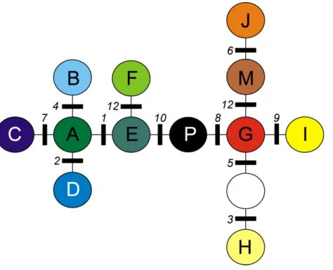
All neighboring chlorotypes were linked by a single mutation (Fig. 1), except for G and H (separated by two mutations). Thus, the MST topology did not allow the division of chlorotypes into clearly demarcated groups separated by more than one mutation.
Chlorotypes did not show equal frequencies in overall sampling (Table 4). The most widely represented was chlorotype J, present in 26.4% of the samples analyzed. Chlorotypes E, F and G had a share of 15.47%, 12.19% and 12.11% respectively. The share of the remaining chlorotypes in the overall sampling was significantly lower than 10%.
Chlorotypes E and J were the most widespread geographically (Fig. 2), with their occurrence established respectively in 6 and 5 out of the 8 investigated geographical regions. Most of the haplotypes occupying tips and terminal branches of the MST were
Figure 1 Minimum spanning tree (MST) presenting relationships between cpDNA haplotypes inA. halleri. Coloured circles represent haplotypes, white circle represent missing haplotype. Numbers indicate mutations as given inTable 2.
more localized geographically. Chlorotypes B, C and H have been found only in the Bohemian Forest, chlorotype D in the Harz Mts., while chlorotype H only in the Eastern Carpathians (Fig. 2). Chlorotype G was found almost exclusively in the Eastern Carpathians, while chlorotype F showed a predominant occurrence in the Western Carpathians as well as in the geographically close region of the Northern Carpathian Foreland.
Genetic diversity indices: chlorotypic richness (ASc) and chlorotype diversity index
(HSd) were calculated for each investigated population. They varied broadly from 1 to
4.983 for AScand from 0 to 0.893 for HSd(Table 4). We also examined the geographical
pattern of variation in chlorotypic richness. As shown inFig. 3, populations with a high level of genetic diversity were co-located in the Bavarian Forest, the Harz Mts. and in the Western Carpathians (Tatra Mts.).
Also we compared genetic diversity indices between different geographical regions (Table 5). As expected, geographical regions differed substantially in terms of genetic diversity. Three regions: Western Carpathians, Harz Mts. and Bohemian Forest were found to be most diverse. The lowest genetic diversity was found in the Alps and in the Sudetes.
Genetic structure
The clustering approach employed in the present study (sphericalk-means clustering—
SKMC) enabled us to study the structure present in our dataset on several levels. We
examined a broad spectrum of differentk values fromk=2 tok=25. The results of
Table 4 Chlorotype distribution among investigated populations ofA. halleriand molecular diversity indices.
Chlorotype
Pop ni A B C D Eα E F G H I J K L M O a7 HSd
A05 14 . . . 14 . . . 1.000 0.000
A08 45 . . . 45 . . . 1.000 0.000
A09 20 . . . 20 . . . 1.000 0.000
CZ04 14 . 13 . . . 1 . . . 1.759 0.143
CZ05 24 . 22 . . . . 2 . . . 1.762 0.159
CZ06 12 . 12 . . . 1.000 0.000
CZ14 20 . . . 20 . . . . 1.000 0.000
CZ16 57 . . . 56 . . . . 1 . . . . 1.231 0.035
CZ18 9 . . . 9 . . . 1.000 0.000
CZ20 33 . . . 11 22 . . . . 1.999 0.458
CZ21 30 . . . 24 6 . . . . 1.972 0.331
CZ22 32 . . . 32 . . . . 1.000 0.000
D01 7 . . 2 . . 4 . . . . 1 . . . . 3.000 0.667
D02 8 2 2 . . 1 . . 1 . 2 . . . . 4.983 0.893
D03 9 2 . . . . 6 . . 1 . . . 2.960 0.556
D04 11 5 . . . . 2 . . 4 . . . 2.990 0.691
D08 12 1 . . 10 . 1 . . . 2.674 0.318
D09 18 3 . . 15 . . . 1.962 0.294
D11 18 5 . . 9 . 4 . . . 2.987 0.660
D12 18 4 . . 6 . 8 . . . 2.989 0.680
D13 20 . . . 17 . 3 . . . 1.940 0.268
D14 11 1 . . 10 . . . 1.879 0.182
PL02 21 . . . 14 . . . 7 . . . . 1.999 0.467
PL03 15 . . . 13 . . . 2 . . . . 1.934 0.248
PL07 19 . . . 4 15 . . . 1.985 0.351
PL08 12 . . . 5 . . . 7 . . . . 2.000 0.530
PL32 27 . . . 11 9 . . 7 . . . 2.992 0.681
PL33 21 . . . 7 . . 14 . . . 1.999 0.467
PL37 40 . . . 40 . . . . 1.000 0.000
PL38 29 . . . 29 . . . . 1.000 0.000
PL39 39 . . . 39 . . . . 1.000 0.000
PL40 39 . . . 39 . . . . 1.000 0.000
PL41 39 . . . 1 38 . . . . 1.329 0.051
PL42 39 . . . 28 11 . . . . 1.994 0.416
PL43 39 . . . 39 . . . . 1.000 0.000
PL44 41 14 . 27 . . . 1.999 0.461
PL45 39 . . . 2 36 . . . 1 . . . . 1.883 0.148
PL46 23 . . . 23 . . . 1.000 0.000
PL47 24 . . . . 4 . . 20 . . . 1.952 0.290
PL48 20 . . . 20 . . . 1.000 0.000
(continued on next page)
Table 4(continued)
Chlorotype
Pop ni A B C D Eα E F G H I J K L M O a7 HSd
PL49 22 . . . . 2 . . 20 . . . 1.798 0.173
PL50 34 . . 34 . . . 1.000 0.000
SK02 22 . . . 4 18 . . . 1.967 0.312
SK05 46 . . . 19 1 . 25 1 . . . . 2.565 0.545
SK10 21 . . . . 7 2 11 . . . 1 . . . . 3.377 0.633
SK12 16 . . . . 7 2 7 . . . 2.915 0.642
UA01 31 . . . . 21 . . 10 . . . 1.998 0.452
UA02 32 . . . . 30 . . 2 . . . 1.638 0.121
UA04 32 . . . . 5 . . 27 . . . 1.932 0.272
UA05 32 . . . . 6 . . 14 . . . 12 . 2.962 0.653
UA06 16 . . . . 1 . . 12 . . . 3 . 2.671 0.425
UA07 8 . . . 6 . . . 2 . 2.000 0.429
Total 1,280 37 47 65 67 83 198 156 155 6 111 338 0 0 17 0 6.927 –
Figure 2 Geographic distribution of cpDNA haplotypes present in the investigated populations ofA. halleri. Bar charts represent the frequency of each haplotype in each investigated population.
Figure 3 Geographic distribution of within-population cpDNA allelic richness (ASc) in the
popula-tions investigated.
Table 5 Comparison of within-population diversity indices among different geographical regions.
Geographical group n ASc HSd
Western Carpathians 5 2.636 0.547
Eastern Carpathians 11 1.895 0.285
Sudetes 12 1.358 0.143
Harz 6 2.405 0.420
Alps 3 1.000 0.000
Bohemian Forest 10 2.169 0.181
N Carpathian Foreland 5 1.960 0.303
Notes.
n, Number of populations in a region;ASc, Chlorotypic richnes;HSd, Chlorotype diversity index.
groups identified by SKMC. Results of SKMC evidenced the presence of some level of genetic admixture in almost all studied geographical regions except in the Harz Mts., the Alps, and the Eastern Carpathians.
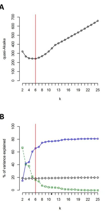
AMOVA performed without grouping populations showed that 79.16% of the total
genetic variation was found between populations (Table 6). When assuming six groups of
populations (according tok-means clustering), as much as 65.8% of the total variation was observed between groups of populations, whereas 15.82% was found among populations within groups (Table 6). These percentages of genetic variation were 42.88% and 37.90%,
Figure 4 Results of sphericalk-means clustering (SKMC).SKMC of investigated populations carried out using Shperikm (Hill, Harrower & Preston, 2013). Statistically optimal level ofk=6 was presented (see Fig. S2for other levels ofk). Different colours (and numbers from 1 to 6) correspond to different clusters identified by SKMC. Population differentiation was inferred from a data matrix of chlorotype frequencies.
respectively, when assuming seven groups (characterised according to the geographical
regions sampled; Table 6). Separate AMOVAs performed within each investigated
geographical region revealed the highest percentage of among-population variation in
the Sudetes and the Bohemian Forest: 85.66% and 74.57%, respectively (Table 6). The
lowest values of among-population variation was found in the Alps, where we recorded the presence of just one chlorotype (0%;Table 6), and in the Harz Mts. (18.55%;Table 6). All the remaining geographic regions showed intermediate level of among-population variation.
Distribution modelling
Model performance was assessed using two different statistics: True Skill Statistic (TSS) and Area under Receiver Operating Characteristic (ROC). All models performed well and had TSS >0.7 and ROC >0.88. The performance of two models CTA and FDA was weaker than the performance of the remaining methods, but still of acceptable quality.
Figure 5 Results of SKMC and AMOVA. (A) Value of the quasi-Akaike information criterion as a function ofk(number of groups identified by SKMC analysis). Statistically optimal solution (having the lowest value of the quasi-Akaike criterion) is marked with a red line. (B) Percent of genetic variance among groups of populations identified by SKMC (blue), among populations within groups (green) and within populations (black) calculated by AMOVA. Statistically optimal solution of SKMC is marked with a red line.
Table 6 Results of AMOVA analysis.All results were significant withα=0.05. Significance tests were carried out using permutation test (10,100
permutations).
Source of variation d.f. Sum of squares Variance
components
Precentage of variation
All populations Among populations 51 1329.890 1.09838 79.16 Within populations 1,233 356.479 0.28912 20.84 Western Carpathians Among populations 5 33.292 0.23835 23.95 Within populations 147 111.244 0.75676 76.05 Eastern Carpathians Among populations 9 32.980 0.14726 46.44
Within populations 230 39.066 0.16985 53.56
Sudetes Among populations 11 408.052 1.01023 85.66
Within populations 427 72.235 0.16917 14.34
Harz Among populations 5 6.934 0.06793 18.55
Within populations 91 27.148 0.29833 81.45
Alps Among populations 2 0.000 0.00000 0.00
Within populations 76 0.000 0.00000 0.00
Bohemian forest Among populations 9 133.130 0.91778 74.57
Within populations 161 50.379 0.31291 25.43
N Carpathian Foreland Among populations 4 18.696 0.20423 26.78
Within populations 101 56.408 0.55849 73.22
k-means clustering (6) Among groups 5 1102.418 1.03618 65.82
Among populations 46 290.472 0.24899 15.82
Within populations 1,233 356.479 0.28912 18.36 Geographic location (7) Among groups 6 759.806 0.64481 42.88
Among populations 45 633.085 0.56992 37.90
Within populations 1,233 356.749 0.28912 19.23
We also analysed the potential distribution ofA. halleriduring the Holocene climatic optimum (ca. 6 kyr BP). Our models showed that recolonization must have advanced very slowly in the Carpathians, when compared with areas north of the Alps. All the models showed that conditions facilitating the spread ofA. hallerioccurred much earlier in between the Western Carpathians, the Sudetes and areas north from the Alps, while suitable areas in the Eastern Carpathians were at first much more restricted (Fig. 6).
DISCUSSION
Carpathian populations of A. halleri
Our data suggest a clear differentiation among populations from western and eastern part of the Carpathians. Those population groups differ in terms of chlorotype composition and frequencies. The same differentiation also appears clearly in the SKMC analysis since the western and eastern populations were grouped in different clusters fromk=2. This pattern of genetic variation seems to follow the division between the eastern and western part of
the Carpathians which was first recognized byWołoszczak (1896)and was established on
Figure 6 Results of modelling experiments.Binary maps of distributions based on the results of ensem-ble models (mean of probabilities) are shown. Results are based on the data from three different paleocli-mate models: CCSM4, MIROC and MPI ESM, as well as current clipaleocli-mate observations. Species range was reconstructed for two time periods: Last Glacial Maximum (LGM, ca. 21 kyr BP) and Mid-Holocene (ca. 6 kyr BP).
Carpathians has been the subject of many studies employing different methodologies from floristic (Pax, 1898;Jasiewicz, 1965) to cytologic (Mráz & Szelag, 2004) and genetic (Mráz et al., 2007;Ronikier, Cieślak & Korbecka, 2008a;Těšitel et al., 2009). It has been hypothesized that specific climatic and orographic conditions of the westernmost part of Bieszczady Mts. (also known as Bukovske Vrchy Mountains) are among the main factors influencing the genetic landscape of this part of Carpathians (Domin, 1940). It seems that results of our study may suggest that differentiation between western and eastern part of Carpathians may be a historical phenomenon connected with recolonisation of the area by plants that survived in different refugia. In this case we do not need to postulate the presence of a specific barrier responsible for the existence of genetic discontinuity between western and eastern part of Carpathians since this phenomenon could be also explained by colonisation from two different directions together with the presence of gene flow between the two groups as was evidenced by our study (i.e., the presence of haplotype P in western and eastern Carpathians).
The Eastern Carpathian populations are characterized by the presence of haplotype G, at very high frequencies. This haplotype was considered as ancestral byPauwels et al. (2005). The presence of the ancestral haplotype G at high frequencies has also been recorded in populations located south of the Alps as well as in the south-eastern part of this mountain range (Pauwels et al., 2012). Our genetic data showing low genetic diversity in the Eastern Carpathians suggest relatively recent recolonisation of this area byA. hallerias was also indicated by the modelling experiments. This is surprising, when we take into account that several studies have demonstrated (with high probablity) that a glacial refugium existed in the Eastern Carpathians (Willis & Van Andel, 2004;Tollefsrud et al., 2008). The low genetic
diversity in the Eastern Carpathians was, however, also confirmed by Tollefsrud et al. (2008)inPicea abies. These authors suggested a genetic bottleneck as a result of substantial decrease in population size as a reason of this phenomenon. The same scenario cannot be ruled out forA. halleri, although modelling experiments carried out during the present study suggest postglacial recolonisation as a more plausible explanation of low genetic diversity in the Eastern Carpathians.
The Western Carpathian populations are characterized by high levels of genetic diversity and the presence of a private haplotype F at high frequencies. Both premises suggest the possibility ofin situglacial survival of the species in the Western Carpathians.
Survival of plant species in the Western Carpathians during the LGM has been a focal point of many studies employing different methodologies. These works have shown that the existence of a Western Carpathian refugium is quite probable for many plant species, including mountain plants. Macrofossil charcoal fragments found in Kraków, just about 30 km in a straight line from population PL8 and about 40 km from PL 7, indicate full glacial presence ofPinus,LarixandAbiesfrom 26 to 28 kyr BP—during the coldest period of LGM that spanned between ca. 36–16 kyr BP (Damblon, Haesaerts & Van der Plicht, 1996;Willis & Van Andel, 2004;Musil, 2003). Dates from humic soil further down in the sequence are even earlier, and indicate the presence of trees as early as 36 kyr BP (Willis & Van Andel, 2004). There is also taxonomic evidence supporting the hypothesis of longstanding survival of different plant species in the Western Carpathians. Saxifraga wahlenbergii
Ball. andDelphinium oxysepalumBorb. et Pax are good examples here. These two species
are endemic to the Western Carpathians and occupy isolated systematic positions, what suggests that they are both of Tertiary age (Mirek & Piekos-Mirkowa, 1992). The survival of
common yew (Taxus baccata), was also documented in charcoal for Moravany in Slovakia
with a radiocarbon date of ca. 18 kyr BP (Lityńska-Zając, 1995). There is also a large body of phylogeographic evidence that indicates the existence of a major northern refugium for a variety of animal taxa in the area around the Carpathians, with some lineages predating LGM (Provan & Bennett, 2008).
On the other hand, results of niche modelling conducted during the present study suggest postglacial recolonization of the area. In this scenario high genetic diversity in the area could be at least partially explained by relatively recent gene flow (occurring later than 6 kyr BP, according to our modelling experiments) from the Eastern Carpathians. The presence of a genetic admixture in Western Carpathian populations was also revealed byPauwels et al. (2012)inA. halleriand byTěšitel et al. (2009)inMelampurum sylvaticum. It seems that the question of the existence of glacial refugium forA. halleriin the Western Carpathians should remain open taking into account that evidence are still not conclusive.
In the SKMC analysis, populations from the Western Carpathians were clustered together with populations from upland regions of southern Poland. This fact supports the hypothesis of a Western Carpathian origin of populations located north of the Western Carpathians. However, for the reasons stated above, it is very difficult to say when these
populations were founded. We have shown that populations ofA. halleriin western and
Carpathians might belong to the group that survived in a southern refugium (areas south of the Alps, Dinaric Alps and Balkan Mts.) as suggested byPauwels et al. (2012).
Genetic differentiation between the Harz, the Bohemian Forest and the Alps
The situation in the areas north and north-east of the Alps is more complex than in the Carpathians. SKMC analysis showed that at least two groups of populations can be recognized regardless of the level of k: populations from the Harz Mountains and from the Alps. Populations from the Bohemian Forest were usually assigned to different clusters, forming very heterogeneous group. This heterogeneity was also evidenced in AMOVA.
Differentiation is also apparent between the regions of the Harz Mts. and the Bohemian Forest, with the first harbouring haplotype D, which is not present in the Bohemian Forest. In the latter region the occurrence of haplotype C can be observed, which, in turn, is present neither in the Harz, nor in the Alps or the Šumava. A relatively recent (postglacial) origin of this differentiation could be hypothesized as both haplotypes occupy external nodes of the MST tree.
It is not easy to explain this pattern of genetic differentiation. Some ideas might be provided by the results published by Tollefsrud et al. (2008). Investigating the genetic variation of Norway Spruce together with pollen data they established that one possible glacial refugium of the species might have extended from the northern slopes of the
Alps up to the Šumava (the Bohemian Massif). It seems that A. hallerimight have also
survived in a vast area, and that its Pleistocene distribution covered not only the region mentioned above, but also extended northwards and westwards to the Ardennes and Hautes Fagnes (High Fens) in Belgium. So far one natural population from this area has been tested byPauwels et al. (2008). This, nowadays isolated, population from Hautes Fagnes, harbouring a chlorotype with an extremely restricted geographical range (Pauwels et al., 2008), might be the trace of a pastA. halleridistribution in Western Europe. The vast extent of possible refugial areas north of the Alps was also clearly evidenced by our modelling experiments. Other studies based on molecular methods also suggest the presence of a glacial refugium in the Central Europe (Reisch, Poschlod & Wingender, 2003;Koch, 2002;
Rejzková et al., 2008).
Genetic variation in the closely related speciesArabidopsis lyratafrom the Harz, southern Germany and the Alps (Clauss & Mitchell-Olds, 2006), can give us some insights into a possible explanation of this pattern. Studies on genetic variation of A. lyrata(carried out on the basis of nuclear microsatellite loci) showed high within-population diversity throughout central Europe, accompanied by low regional differentiation and geographically widespread polymorphism. The authors hypothesized that (given the unlikeliness of gene flow) a common gene pool must have existed for central European populations (Koch & Matschinger, 2007). It should be noted that ‘‘central European’’ in this case is not a precise term and describes sites located approximately between the 10th and 16th eastern meridian. This area corresponds to the locations of the populations sampled by us north of the Alps in the the Bohemian Forest and the Harz. The same scenario is also probable forA. halleri, where haplotype E, present in all regions north of the Alps, can be interpreted as a testimony
to a common gene pool in the past. Other haplotypes, with restricted geographical range, would be, under this model, local derivatives that evolved after climatic warming and fragmentation of a previously vast range.
The Bohemian Forest hosts a population with the highest genetic diversity in the whole sampled area. The question whether this high genetic diversity should be attributed to the existence of a glacial refugium in this region or the presence of a contact zone between eastern and western lineages remains open. We think that results cited above (Clauss & Mitchell-Olds, 2006;Tollefsrud et al., 2008) as well as data clearly suggesting the presence of a glacial refugium forFagusin the southern part of Czech Republic (Magri et al., 2006) make the hypothesis of the existence of a glacial refugium in this area more probable. The fact
that even nowadays the range ofA. halleriand Norway Spruce in Central Europe is highly
similar (Tollefsrud et al., 2008) also suggest this scenario. However, no palaeobotanical data are available for A. halleri. Therefore, such a hypothesis cannot be fully confirmed or rejected. It should be also noted that the area between the 10th and 16th eastern meridian has been identified as a contact zone for some plant species (Fjellheim et al., 2006;
Daneck et al., 2011). It is clear that further detailed studies in this region, also including other taxa, are needed to clarify these findings more precisely.
Origin ofA. halleri populations in the Sudetes
We have shown that A. halleripopulations in Sudetes are characterized by a very low
genetic variation, with most of the populations harbouring only one cpDNA haplotype. This finding is not surprising, given the evidence from geological research showing that this region was severely impacted during the glacial period. Is seems that at least one glacial maximum (48–43 kyr BP) had a devastating effect on the regional flora, mainly due to the close proximity of the continental ice sheet (Marks, 2005). Geological evidence show that even during LGM this region was affected by the presence of the mountain glaciers (Badura & Przybylski, 1998). Therefore, it has been postulated thatin situglacial refugia, supporting the remains of the autochthonous flora, did not exist in the Sudetes (Mitka et al., 2007). Quite a different scenario involving survival on nunataks and in peripheral refugia has been suggested for the Alps (Stehlik, 2000). It is noteworthy that even nowadays the climate of the highest parts of the Sudetes is cold enough to maintain the occurrence of tundra-like ecosystems (Soukupova et al., 1995) . It seems therefore, thatA. halleripopulations in the Sudetes could be of a recent (postglacial) origin. This is supported by the very low genetic variation found in Sudetes as well as the fact that despite dense sampling, we have not found any chlorotypes specific to this area. On the basis of the evidence from cpDNA variation, it could be hypothesized that populations from the Bohemian Forest could be a source of migrants that established new populations of the species in this region after LGM.
We have also found the presence of haplotype I in high-mountain populations of
the past.Mitka et al. (2007)suggested that this contact could have occurred especially for high-mountain taxa, which could easily disperse within the open landscapes that were present between the Sudetes and the Carpathians during glacial maxima. This supposition is also supported by the floristic evidence showing that several high-mountain taxa such as Erigeron macrophyllusHerbich,Melampyrum herbichii Woł.,Sesleria tatrae (Degen)
Deyl and Thymus carpathicusČelak. that are present in the Carpathians, occur also in
high-mountain environments of the Sudetes (Pawłowski, 1969). The connections between
the Carpathian and Sudetic populations ofA. hallerisurely require further studies.
Taxonomic concept of A. halleri in the Carpathians
Taxonomy of A. halleriis still much debated and to date three European subspecies
have been recognised: subsp. halleri, subsp.tatrica (Pawł.) Kolník, and subsp.dacica
(Heuff.) Kolník (Hohmann et al., 2014). This division is based on a morphological study of the Carpathian populations published byKolník & Marhold (2006). Our results seem to question this taxonomic division that has already been cited by various authors (Clauss & Mitchell-Olds, 2006; Koch, Wernisch & Schmickl, 2008). We have shown that main genetic groups identified by cpDNA variation are not consistent with the division proposed byKolník & Marhold (2006), nor with the distribution of the described taxa.
CONCLUSIONS
1. Genetic variation in A. halleri is strongly geographically structured within the investigated area and at least 6 clusters of populations can be identified on the basis of cpDNA variation.
2. There is a clear genetic differentiation within the Carpathian populations. Two distinct clusters of populations were identified in western and eastern part of the mountain range. It is clear that the two groups originated from two different glacial refugia. There are traces of gene flow between the two groups.
3. The possibility of the existence of a glacial refugium in the Western Carpathians and the Bohemian Forest cannot be ruled out on the basis of the present research but the evidence is not conclusive.
4. It seems that the area of Sudetes was colonised after LGM. Populations from the
Bohemian Forest can be hypothesised as a source of the migrants which establishedA.
halleripopulations in the area.
ACKNOWLEDGEMENTS
The authors would like to thank Prof. Ian C. Trueman (University of Wolverhampton, UK) for improving the English of the manuscript. Krkonošský národní park (CZ), Karkonoski Park Narodowy (PL), Tatrzański Park Narodowy (PL), Bieszczadzki Park Narodowy (PL) and Karpatskij biosfernij Zapovidnik (UA) are acknowledged for granting permits to collect plant samples within protected areas of these national parks.
ADDITIONAL INFORMATION AND DECLARATIONS
Funding
The study was founded by grants from: Polish Ministry of Science and Higher Education N303415336 and Égide (Campus France) 7298/R08/R09. The funders had no role in study design, data collection and analysis, decision to publish, or preparation of the manuscript.
Grant Disclosures
The following grant information was disclosed by the authors: Polish Ministry of Science and Higher Education: N303415336. Égide (Campus France): 7298/R08/R09.
Competing Interests
The authors declare they are no competing interests.
Author Contributions
• Pawel Wasowicz conceived and designed the experiments, performed the experiments,
analyzed the data, contributed reagents/materials/analysis tools, wrote the paper, prepared figures and/or tables, reviewed drafts of the paper.
• Maxime Pauwels conceived and designed the experiments, performed the experiments,
contributed reagents/materials/analysis tools, wrote the paper, reviewed drafts of the paper.
• Andrzej Pasierbinski conceived and designed the experiments, performed the
experiments, analyzed the data, contributed reagents/materials/analysis tools, prepared figures and/or tables, reviewed drafts of the paper.
• Ewa M. Przedpelska-Wasowicz performed the experiments, analyzed the data,
contributed reagents/materials/analysis tools, prepared figures and/or tables, reviewed drafts of the paper.
• Alicja A. Babst-Kostecka performed the experiments, contributed
reagents/materials/-analysis tools, reviewed drafts of the paper.
• Pierre Saumitou-Laprade and Adam Rostanski conceived and designed the experiments,
performed the experiments, contributed reagents/materials/analysis tools, reviewed drafts of the paper.
Field Study Permissions
The following information was supplied relating to field study approvals (i.e., approving body and any reference numbers):
Data Availability
The following information was supplied regarding data availability:
Raw data—chlorotype frequencies in each population—can be found inTable 4.
Supplemental Information
Supplemental information for this article can be found online athttp://dx.doi.org/10.7717/ peerj.1645#supplemental-information.
REFERENCES
Al-Shehbaz IA, O’Kane SL. 2002.Taxonomy and phylogeny ofArabidopsis(Brassicaceae).
The Arabidopsis Book1:e0001DOI 10.1199/tab.0001.
Alvarez N, Thiel-Egenter C, Tribsch A, Holderegger R, Manel S, Schönswetter P, Taber-let P, Brodbeck S, Gaudeul M, Gielly L, Küpfer P, Mansion G, Negrini R, Paun O, Pellecchia M, Rioux D, Schüpfer F, Van Loo M, Winkler M, Gugerli F. 2009. History or ecology? Substrate type as a major driver of spatial genetic structure in Alpine plants.Ecology Letters12(7):632–640DOI 10.1111/j.1461-0248.2009.01312.x.
Badura J, Przybylski B. 1998.Zasięg lądolodów plejstoceńskich i deglacjacja obszaru
pomiędzy Sudetami a Wałem Śląskim.Biuletyn Państwowego Instytutu Geologicznego
385:9–28.
Barbet-Massin M, Jiguet F, Albert CH, Thuiller W. 2012.Selecting pseudo-absences
for species distribution models: how, where and how many?Methods in Ecology and
Evolution3(2):327–338DOI 10.1111/j.2041-210X.2011.00172.x.
Clauss MJ, Mitchell-Olds T. 2006.Population genetic structure ofArabidopsis lyratain
Europe.Molecular Ecology15(10):2753–2766
DOI 10.1111/j.1365-294X.2006.02973.x.
Daneck H, Abraham V, Fér T, Marhold K. 2011.Phylogeography ofLonicera nigrain
Central Europe inferred from molecular and pollen evidence.Preslia83:237–257.
Damblon F, Haesaerts P, Van der Plicht J. 1996.New datings and considerations on
the chronology of Upper Palaeolithic sites in the Great Eurasiatic Plain.Prehistoire Europeenne9:177–231.
Despres L, Loriot S, Gaudeul M. 2002.Geographic pattern of genetic variation in the
European globeflowerTrollius europaeusl. (Ranunculaceae) inferred from amplified
fragment length polymorphism markers.Molecular Ecology11(11):2337–2347.
Domin K. 1940.O geobotanickem rozhraní Zapadních a Vychodních Karpat.Veda
Prírodní 20:76–78.
Dormann CFC, Elith J, Bacher S, Buchmann C, Carl G, Carré G, Marquéz JRG, Gruber B, Lafourcade B, Leitão PJ, Münkemüller T, Mcclean C, Osborne PE, Reineking
B, Schröder B, Skidmore AK, Zurell D, Lautenbach S. 2013.Collinearity: a review
of methods to deal with it and a simulation study evaluating their performance.
Ecography36:27–46DOI 10.1111/j.1600-0587.2012.07348.x.
Ehlers J, Eissmann L, Lippstreu L, Stephan HJ, Wansa S. 2004. Pleistocene glaciations
of North Germany. In: J Ehlers, PL Gibbard, eds.Quaternary glaciations extent and chronology—Part I: Europe. Amsterdam: Elsevier, 135–146.
El Mousadik A, Petit R. 1996.High level of genetic differentiation for allelic richness
among populations of the argan tree endemic to Morocco.Theoretical and Applied
Genetics7(92):832–839DOI 10.1007/BF00221895.
Excoffier L, Laval G, Schneider S. 2005.Arlequin ver. 3.0: an integrated software package
for population genetics data analysis.Evolutionary Bioinformatics Online1(1):47–50.
Excoffier L, Smouse PE. 1994.Using allele frequencies and geographic subdivision to
reconstruct gene trees within a species: molecular variance parsimony.Genetics
136:343–359.
Fjellheim S, Rognli OA, Fosnes K, Brochmann C. 2006.Phylogeographical
his-tory of the widespread meadow fescue (Festuca pratensishuds.) inferred from
chloroplast dna sequences.Journal of Biogeography33(0318):1470–1478
DOI 10.1111/j.1365-2699.2006.01521.x.
Goudet J. 2013.FSTAT: a computer program to calculate F-Statistics.Journal of Heredity
104:586–590DOI 10.1093/jhered/est020.
Hewitt G. 1999.Post-glacial re-colonization of European biota.Biological Journal of the
Linnean Society68(1-2):87–112DOI 10.1111/j.1095-8312.1999.tb01160.x.
Hewitt GM. 2000.The genetic legacy of the quarternary ice ages.Nature405:907–913
DOI 10.1038/35016000.
Hewitt GM. 2004.Genetic consequences of climatic oscillations in the Quaternary.
Philosophical transactions of the Royal Society of London. Series B, Biological sciences
359(1442):183–195DOI 10.1098/rstb.2003.1388.
Hijmans RJ, Cameron SE, Parra JL, Jones PG, Jarvis A. 2005.Very high resolution
in-terpolated climate surfaces for global land areas.International Journal of Climatology
25(15):1965–1978DOI 10.1002/joc.1276.
Hill MO, Harrower CA, Preston CD. 2013.Sphericalk-means clustering is good for
interpreting multivariate species occurrence data.Methods in Ecology and Evolution
4(6):542–551DOI 10.1111/2041-210X.12038.
Hohmann N, Schmickl R, Chiang T-Y, Lu Anová M, Kolá F, Marhold K, Koch M. 2014.
Taming the wild: resolving the gene pools of non-modelArabidopsislineages.BMC
Evolutionary Biology14(1):224DOI 10.1186/s12862-014-0224-x.
Jalas J, Suominen J. 1994.Atlas Florae Europaeae. Distribution of Vascular Plants in
Europe. 10. Cruciferae (Sisymbrium to Aubertia). Helsinki: The Committee for Mapping the Flora of Europe and Societas Biologica Fennica Vanamo.
Jasiewicz A. 1965.Rośliny naczyniowe Bieszczadów Zachodnich.Monographiae
Botani-cae22:1–340.
Jiménez-Valverde A, Lobo JM. 2007.Threshold criteria for conversion of probability
of species presence to either-or presence-absence.Acta Oecologica31(3):361–369
DOI 10.1016/j.actao.2007.02.001.
Kalinowski ST. 2004.Counting alleles with rarefaction: private alleles and hierarchical
sampling designs.Conservation Genetics5(4):539–543
DOI 10.1023/B:COGE.0000041021.91777.1a.
Koch M. 2002.Genetic differentiation and speciation in prealpineCochlearia:
Cochlearia pyrenaicaDC. in Germany and Austria.Plant Systematics and Evolution
232(1–2):35–49DOI 10.1007/s006060200025.
Koch M, Matschinger M. 2007.Evolution and genetic differentiation among relatives
ofArabidopsis thaliana.Proceedings of the National Academy of Sciences of the United States of America104(15):6272–6277DOI 10.1073/pnas.0701338104.
Koch M, Wernisch M, Schmickl R. 2008.Arabidopsis thaliana’s wild relatives: an
updated overview on systematics, taxonomy and evolution.Taxon57(3):933–943.
Kolník M, Marhold K. 2006.Distribution, chromosome numbers and
nomencla-ture conspect ofArabidopsis halleri(Brassicaceae) in the Carpathians.Biologia
61(1):41–50DOI 10.2478/s11756-006-0007-y.
Lityńska-Zając M. 1995. Anthracological analysis. In: Hromada J, Kozłowski J, eds.
Complex of Upper Palaeolithic sites near Moravany Western Slovakia. Wydawnictwo Uniwersytetu Jagiellońskiego, 74–79.
Llaurens V, Castric V, Austerlitz F, Vekemans X. 2008.High paternal diversity
in the self-incompatible herbArabidopsis halleridespite clonal reproduction and spatially restricted pollen dispersal.Molecular Ecology 17(6):1577–1588
DOI 10.1111/j.1365-294X.2007.03683.x.
Magri D, Vendramin GG, Comps B, Dupanloup I, Geburek T, Gömöry D, Latałowa M, Litt T, Paule L, Roure JM, Tantau I, Van Der Knaap WO, Petit RJ, De Beaulieu
JL. 2006.A new scenario for the Quaternary history of European beech
pop-ulations: palaeobotanical evidence and genetic consequences.New Phytologist
171(1):199–221DOI 10.1111/j.1469-8137.2006.01740.x.
Marks M. 2005.Pleistocene glacial limits in the territory of Poland.Przegląd Geologiczny
53:988–993.
Médail F, Diadema K. 2009.Glacial refugia influence plant diversity patterns in the
Mediterranean basin.Journal of Biogeography36(7):1333–1345
DOI 10.1111/j.1365-2699.2008.02051.x.
Mirek Z, Piekos-Mirkowa H. 1992.Flora and vegetation of the Polish Tatra Mountains.
Mountain Research and Development 12(2):147–173DOI 10.2307/3673788.
Mitka J, Sutkowska A, Ilnicki T, Joachmiak A. 2007.Reticulate evolution of high-alpine
Aconitum(Ranunculaceae) in the Eastern Sudetes and Western Carpathians (Central Europe).Acta Botanica Cracoviensia Series Botanica49:15–26.
Mráz P, Gaudeul M, Rioux D, Gielly L, Choler P, Taberlet P. 2007.Genetic structure of
Hypochaeris uniflora(Asteraceae) suggests vicariance in the Carpathians and rapid post-glacial colonization of the Alps from an eastern Alpine refugium.Journal of Biogeography 34(12):2100–2114DOI 10.1111/j.1365-2699.2007.01765.x.
Mráz P, Szelag Z. 2004.Chromosome numbers and reproductive systems in selected
species ofHieraciumandPilosella(Asteraceae) from Romania.Annales Botanici Fennici41:405–414.
Musil R. 2003. The middle and upper palaeolithic game suite in Central and
South-Eastern Europe. In: Van Andel T, Davies S, eds.Neanderthals and modern humans
in the European landscape during the last glaciation. Cambridge: McDonald Institute for Archaeological Research, 167–190.