PREDICTION OF AEROSOL HAZARDS ARISING FROM THE OPENING OF AN ANTHRAX-TAINTED LETTER IN AN OPEN OFFICE ENVIRONMENT USING COMPUTATIONAL FLUID DYNAMICS

!" # $ " % &

'#

( ) *+

-#( +

#)

.

/+** 01#2 +0(0+

1_{Department of Mechanical and Mechatronics Engineering, University of Waterloo,}

Waterloo, ON, N2L 3G1, Canada

2

Waterloo CFD Engineering Consulting Inc.534 Paradise Crescent, Waterloo, ON, N2T 2N7, Canada

3

Defence R&D Canada – Suffield, P.O. Box 4000 STN MAIN, Medicine Hat, AB, T1A 8K6, Canada

*Corresponding Author: fslien@uwaterloo.ca

Early experimental work, conducted at Defence R&D Canada–Suffield, measured and characterized the personal and environmental contamination associated with simulated anthrax=tainted letters under a number of different scenarios in order to obtain a better understanding of the physical and biological processes for detecting, assessing, and formulating potential mitigation strategies for managing the risks associated with opening an anthrax=tainted letter. These experimental investigations have been extended in the present study to simulate numerically the contamination from the opening of anthrax= tainted letters in an open office environment using computational fluid dynamics (CFD). A quantity of 0.1 g of (formerly referred

to as (BG)) spores in dry powder form, which was

used here as a surrogate species for (anthrax), was released from an opened letter in the experiment. The accuracy of the model for prediction of the spatial distribution of BG spores in the office from the opened letter is assessed qualitatively (and to the extent possible, quantitatively) by detailed comparison with measured BG concentrations obtained under a number of different scenarios, some involving people moving within the office. The observed discrepancy between the numerical predictions and experimental measurements of concentration was probably the result of a number of physical processes which were not accounted for in the numerical simulation. These include air flow leakage from cracks and crevices of the building shell; the dispersion of BG spores in the Heating, Ventilation, and Air Conditioning (HVAC) system; and, the effect of deposition and re=suspension of BG spores from various surfaces in the office environment.

Concentration, g/m

Time=averaged concentration, g/m

Measured concentration value, g/m

Turbulence kinetic energy, m

/s

ON

Tracer release period, s

Time, s

ε

Dissipation rate of turbulence kinetic energy, m

/s

Time step, s

A, B, C

Sampler locations, Fig. 1

LO

Location of letter opener, Fig. 11

SKC

Location of SKC samplers, Fig. 11

ACPLA

Agent containing particles per liter of air

BG

(formerly known as

)

CBW

Chemical and biological warfare

CFD

Computational fluid dynamics

CFM

Cubic feet per minute

CFU

Colony forming unit

CW

Co=worker

DRDC

Defence R&D Canada

EIM

Eddy interaction model

GCIBM

Ghost=cell immersed boundary method

HR

High=resolution slit samplers

HVAC

Heating, ventilation, and air conditioning

IBM

Immersed boundary method

LO

Letter opener

LR

Low=resolution slit samplers

NIOSH

National institute for occupational safety and health

QUICK

Quadratic upstream interpolation for convective kinematics

RANS

Reynolds=averaged Navier=Stokes

SIMPLE Semi=implicit method for pressure=linked equations

TVD

Total variation diminishing

UMIST

Upstream monotonic interpolation for scalar transport

6

use of chemical and biological warfare (CBW) agent weapons against civilian

populations in dense urban centers. In previous experimental work [2=5], Defence

R&D Canada–Suffield (DRDC–Suffield) measured and characterized the

personal and environmental contamination associated with simulated anthrax=

tainted letters under a number of different scenarios, in order to obtain a better

understanding of the physical and biological processes for detecting, assessing,

and formulating potential mitigation strategies for managing the risks associated

with opening an anthrax=tainted letter. These experimental investigations in

multiple small offices have been extended to characterize the contamination from

anthrax=tainted letters in an open office environment. In a related study, Price et

al. [6] investigated recently the risk to occupants in a building resulting from re=

suspension of deposited anthrax spores on indoor surfaces.

Practical mathematical models for prediction of dispersion of anthrax spores

from opened letters in an indoor environment, which include the effects of

people moving in the various offices on the dispersion, do not exist owing to the

inherent complexity of the problem. There are an enormous number of possible

scenarios for incidents involving anthrax=tainted letters due to their deliberate

nature. Furthermore, the physical insight and concomitant data necessary to

perform and validate the model predictions for most scenarios involving

anthrax=tainted letters are (until recently) rather limited. In addition, the

parameters required by the model (e.g., deposition velocity of anthrax spores on

various types of surfaces) and the data needed to infer these parameters are not

available. In spite of these complications, Reshetin and Regens [7] developed a

box model to investigate the dispersion of anthrax spores released in a high=rise

building. Following from this work, we will show in the present study that a

more sophisticated modeling approach based on computational fluid dynamics

(CFD) is able to make credible predictions of both the flow characteristics

inside buildings (and, more specifically in an office within a building) and the

concomitant dispersion of contaminants (e.g., anthrax spores from an opened

letter) released into these flows.

The objective of the present study is to undertake a critical assessment of the

utility of current CFD models for the prediction of flow and dispersion in the

indoor environment. In particular, CFD modeling of the dispersion of a

biological simulant

[formerly known as

(BG)] for anthrax, released from an opened letter in a large office (open

office concept), will be undertaken. The accuracy of the model for prediction of

the spatial distribution of BG spores in the office will be assessed qualitatively

(and to the extent possible, quantitatively) by detailed comparison with

measured BG spore concentrations obtained under a number of scenarios. In

Section 2, the basic numerical framework for the CFD model used for these

numerical studies, including the capability for simulating the movement of

people in an office will be described. Section 3 will compare predictions against

a baseline experiment in which a tracer gas (sulfur hexafluoride, or SF

) was

The STREAM code [8] was used in the present study for our numerical

simulations. STREAM is a fully=conservative, block=structured finite=volume

code for computational fluid dynamics, which employs a fully=collocated storage

arrangement for all transported properties, including various turbulence quantities

(e.g., turbulence kinetic energy, viscous dissipation rate, etc.). Within an arbitrary

non=orthogonal coordinate system, the velocity vector is decomposed into its

Cartesian components, and these are the components to which the momentum

equations relate. Advective cell=face fluxes are approximated by the Upstream

Monotonic Interpolation for Scalar Transport (UMIST) scheme [9], obtained by

formally imposing Total Variation Diminishing (TVD) constraints on Leonard’s

third=order accurate Quadratic Upstream Interpolation for Convective Kinematics

(QUICK) scheme [10]. A second=order fully implicit three=level scheme is used

to treat the transient (or, local tendency) term. The mass continuity is enforced by

solving a pressure=correction equation using the Semi=Implicit Method for

Pressure=Linked Equations (SIMPLE) algorithm, which steers, as part of the

iterative sequence, the pressure towards a state in which the mass residuals in all

cells of the flow domain are negligibly small.

All transport equations, including mean momentum, turbulence and scalar

concentration equations, are discretised and solved sequentially as part of the

SIMPLE algorithm [11]. The linearized and discretised equations obtained in the

outer iterations of the SIMPLE algorithm are solved numerically using very

efficient iterative linear equation solvers, such as Stone’s Strongly Implicit

Procedure (SIP3D) [12] or the Conjugate Gradient Stabilized (CGSTAB) method.

In conjunction with a fully=collocated approach, the SIMPLE algorithm is known

to provoke checkerboard oscillations in the pressure field, reflecting a state of

velocity=pressure decoupling. To avoid this, the widely used method of Rhie and

Chow [13] has been adopted to interpolate the cell=face velocities from the

adjacent nodal values. This interpolation essentially introduces a fourth=order

“pressure smoothing” to remove the checkerboard oscillations in the pressure

field. Physical diffusion fluxes are approximated using a conventional second=

order accurate central differencing approach.

For mesh generation, the “ray=casting” approach [14] is used to determine

whether a computational cell lies inside the complex geometry of objects

encountered in the current problem, such as desks, partitions, and people in the

study area. If the cell centroid is inside an object, the flag associated with this cell

will be set to OBJECT. Otherwise, the cell flag is set to FLUID, allowing an

efficient matrix solver (e.g., SIP3D) to be utilized for the solution of the

discretised equations.

7

function) was used to interpolate and extrapolate information between the

immersed boundary and the background grid. Unfortunately, the use of the

cosine=function formulation smeared out the solution over a thin finite band

centered on the boundary, which in general could have an adverse effect on the

solution accuracy. Furthermore, IBM may induce spurious oscillations and,

consequently, restricted severely the size of the computational time step,

especially when an explicit time=integration method was used for the flow solver.

To overcome these difficulties, other IBM variants such as the ghost=cell

immersed boundary method (GCIBM) [16], have been proposed. In contrast to

IBM, GCIBM uses ghost cells within the solid objects as boundary conditions,

without having to explicitly introduce a forcing term into the mean momentum

equation. The ghost cells are reconstructed using either linear or quadratic

interpolation of the property values at the neighbouring fluid nodes in the physical

domain and at the boundary node. Although IBM has been widely used, most

previous researchers have incorporated it into explicit flow solvers based on a

fractional=step method, which as mentioned above severely limits the maximum

allowable time step that could be used for the integration. Moreover, very little

work has been undertaken to date, to combine IBM with a high=Reynolds=number

Reynolds=averaged Navier=Stokes (RANS) solver for turbulent flow problems. In

the present study, we have successfully incorporated the GCIBM into STREAM

to give a fully implicit time=stepping scheme that utilizes a standard =ε

turbulence model, in conjunction with wall functions as boundary conditions at

the solid surfaces (e.g., walls). This advancement in the application of GCIBM

permitted the simulation of moving boundaries corresponding to mobile objects

(e.g., people) within the flow domain.

! "

# $

Five tracer gas experiments [17], involving the release of SF

, were conducted by

personnel from the National Institute for Occupational Safety and Health

(NIOSH). These experiments were undertaken in a simulated open office complex

(see Fig. 1) set up in Building 13 on the DRDC–Suffield campus. Furthermore,

NIOSH personnel also measured the flow rates of all the supply and return ducts

[in cubic feet per minute (CFM)] in this study area. The latter information was

used to specify the inflow/outflow boundary conditions for our CFD simulations.

For comparisons with our numerical simulations, only data from “Experiment 1”

will be used. In this experiment, 2.5 liters of pure SF

was released over a short

period of several seconds from an airtight syringe at location F (letter=opener

position) in Fig. 1. Measurements of the time history of the SF

concentration in

parts per million by volume (ppm) were made at six locations (namely, at

locations A, B, C, D, E, and G) as shown in Fig. 1.

Because the dispersion of SF

in the study area is strongly influenced by the

8

side of Fig. 3. We expect to see a clockwise vortex flow motion in a vertical =

plane that contains the discharging jet from one of the air supply ducts flush=

mounted on the floor. The implication of this figure is that the flow motion in a

selected = plane that contains an air supply duct can be quite energetic,

contrasting with the fact that the flow motion in the =direction is actually rather

weak. This can be seen clearly in Fig. 4, which exhibits stream traces near the

front part of the study area. We should note that the average velocity from the

supply and return ducts is about 1 m s

. The magnitude of the average velocity in

the study area is about 0.05 m s

_{. The average velocity in the =direction is}

approximately −0.002 m s

, which confirms the above=mentioned assertion of a

weak flow motion in the =direction.

%

&

'

%

( %

)

*

$$ &

"

+

,

"

)

)

!

$

% )

)

, ', -, +, #,

.!

/

.

0

# $

(

%

.

.

&

& - +

9

%

*

2

*

2

3 *

# $

% 4 *

/

)

1$

)1!

# $

The release period for the SF

tracer is assumed to be

= 10 s in the CFD

simulation, although a release period of 5 s was also simulated with little

observed effect on the final solution. In order to increase the time accuracy of the

numerical prediction, the time step, , for the simulation was chosen as follows:

R = 0.2 s for ≤

; R = 2 s for

< < 120 s; and, R = 10 s for ≥ 120 s.

The total time for the simulation is 7200 s after the initial release of the SF

tracer.

The predicted time histories of the mean concentration of SF

at locations A, B,

:

release of the SF

tracer). This peak concentration occurs much earlier than that

predicted by the numerical simulation at the same location, where the predicted

peak value of concentration is seen to be 10 ppm occurring at = 780 s (13 min).

Similarly, the experimental concentration measurements at location B (where co=

worker 2 is collocated) achieves a peak concentration value of 11 ppm at = 300 s

(5 min). This needs to be compared with the predicted peak concentration value

of 6 ppm at the time = 3000 s (50 min) at this location. Again, the peak

concentration value is under=predicted and occurs at a much later time

!'" ('! )

* (+ + ' ) ( ;3% / ;3% & ;3% < ;3% ;3% ) ;3%

;3

4

%

% 5 /

-

$$

- + *

-

$

(

# $

# $

In order to identify what might be the cause of the discrepancy in the predicted

and observed cloud arrival times, two additional simulations were conducted.

Firstly, a simulation was conducted for the same test problem using a finer mesh

of 140×100×70 nodes to investigate the effects of grid resolution on the fidelity of

the prediction. It was found that this higher=resolution simulation gave essentially

the same results as the original simulation, implying that grid resolution was not

responsible for the discrepancy between the predicted and observed tracer

concentration. Secondly, a simulation was conducted in which the direction of air

flow at each supply duct location was deflected by grills at ±45° (in contrast to

the original simulation in which the air flow from the supply duct was assumed to

be in the vertical =direction). Again, no major changes were observed in the

predicted results.

In light of this, the discrepancy between the predicted and observed SF

concentration=time histories may be due to one or more of the following causes:

•

In the actual situation, SF

released from location F can enter the return

(1=D)” in the sense that they treat each room in a building as a well=

mixed zone and, consequently, cannot be applied to the simulation of the

complex 3=D flow and dispersion in a large office with furniture. The

remedy for this problem is to develop a general procedure, which can

couple the present CFD model (used to simulate the 3=D indoor flow and

dispersion in the study area) with one of the zonal models (which can be

used to simulate the flow and dispersion in the HVAC system, the latter

of which is simply treated as a well=mixed zone).

•

Building 13 on the DRDC–Suffield campus is an old vacated office

building. The envelope or shell of this building is very leaky.

Consequently, flow through cracks and crevices in the building envelope

(e.g., window sills, walls, etc.), which have not been accounted for in our

simulations, will undoubtedly generate additional air motions in the

office. These air motions can significantly alter the dispersion of the SF

tracer in the office. To incorporate the effects of building leakage in our

simulations, a “blower door” experiment will need to be conducted in

order to identify the locations of the leakage points and to measure the

flow rate through these points. With this additional information, it is

conceivable that the predictive accuracy of our current CFD simulation

results will be improved.

In addition to the two reasons enunciated above, anomalies in the experiment

can also contribute to the observed discrepancy between the CFD predictions and

the experimental measurements. To see this, let us also examine the results of

Experiment 5 from the SF

release experiments [17], which are shown in Fig. 6.

The major differences between Experiments 1 and 5 are as follows: in Experiment

1, pure SF

was released from an air=tight syringe for a release period of 30 s,

whereas Experiment 5 involved the release of dilute SF

from a sampling pump

for a release period of 60 s. Note that in Experiment 5, a dilute mixture consisting

of one liter of pure SF

and 3 litres of air was used. Nevertheless, in spite of the

differences in source strength in Experiments 1 and 5, the relative ratios of peak

mean concentrations at locations A, B and D for each experiment should be the

same (assuming that the nominal conditions in the office were unchanged

between these experiments).

It is seen from Figs. 5 and 6 that (

:

:

)

≈ (6.75 : 3.7 : 1) for

Experiment 1 and (

:

:

)

≈ (22.7 : 1.1 : 1) for Experiment 5, where

denotes the concentration and the subscript on indicates the location where the

concentration was measured. In our current simulation, (

:

:

)

≈ (1.75 :

1 : 1). If we simply focus on (

/

)

, we find that (

/

)

≈ 1.1 from

Experiment 5 is very close to our current prediction of (

/

)

≈ 1, which is

encouraging. This seems to suggest that the much larger value of

% /

.

# $

56

)

6

*

/

(

"

"

0

%

$

% *

$

With reference to Fig. 6, the “well=mixed” condition for which concentration

levels at all sampler locations are very similar, is clearly shown to be achieved

(approximately or better) when = 3000 s (50 min) in Experiment 1. However,

even after 7200 s, the well=mixed condition was not achieved in our numerical

simulation, particularly at locations A (co=worker 1) and E (sampler in Area IV),

which is consistent with the iso=surfaces of concentration (ppm) at = 180, 1200

and 7200 s (after the release) as shown in Figs. 7 to 9.

% 7

3

*

-

$$

% 9

3

*

-

$$

- + *

8 :

# $

% ;

3

*

-

$$

- + *

8

:

# $

Experiment 1 is less satisfactory, a result that is probably due to air flow leakage

through the building envelope among other things, recommendations aimed at

improving the present predictive results will be made in Section 5.

=

;

#₅

=

; >

>

: > 7 >

%

: /

&

*

<

-

*

<

&

-

!

2

-

*

8 :!

1

&

%

=

8 : 75

+

)

6 *

> +

3

)

6 # $

? :@

4

'.! "

# $

6

4

: '

-

!

A source of 0.1 g of BG spores in powder form was placed in a sealed envelope.

This envelope was located at the position occupied by the LO (Letter Opener), as

shown in Fig. 11. To simplify the notation henceforth, Co=worker 1 and Co=

worker 2 in Fig. 11 will be referred to as CW1 and CW2, respectively. The LO

(person) was positioned about 0.5 m in front of the source location (sealed

envelope containing the BG spores). The office geometry and grid, consisting of

116×74×30 nodes in the =, = and =directions, respectively, are shown in Fig. 12.

Note that the major differences between Figs. 2 and 12 are that partitions were

added between the various desks in the study area, and the two middle doors in

Area I (Fig. 12) were closed. The HVAC system was turned on for about 15 min

until the flow reaches a pseudo=steady state condition before the sampling process

began. The sampling process lasted for 30 min. During the sampling stage, the

HVAC was still on, and the front and rear doors in Area I were open. As for the

SF

experiment described earlier, BG spores entering the return ducts were

assumed to be released directly to the outdoor environment (viz., no spores

entering the return ducts were allowed to re=enter the study area through the

supply ducts) in the present simulations. The (unknown) effects of deposition and

re=suspension of BG spores in the study area were not considered here (viz., walls

and other surfaces in the open office were assumed to be perfect reflectors in the

sense that no BG spores were deposited on these surfaces). Immediately after the

BG spores were released (viz., after the letter was opened), the LO remained

stationary for the remainder of the test period. The total release time for the BG

spores was assumed to be 10 s.

%

&

'

%

( %

) &

, )

$$ &

"

,

"

$

% )

%

.

.

& 0

& - +

'. "

# $

Contours of log

(100 ), where is the concentration in g/m

3

, are shown in

Fig. 13 at = 8.75 s and in Fig. 14 at = 1800 s (30 min). Note that the presence

of the LO in Fig. 14 obstructs the spread of the BG spores. Concentration

contours in Fig. 14 suggest that BG spores have already dispersed into the entire

study area at = 1800 s (30 min), with concentrations in regions in or close to

Area IV being the smallest. The unit for the predicted concentration “ ’ shown in

Figs. 15, 16 and 18 is g/m

. This is different than the unit of measured

concentration used in Fig. 19 (namely, Agent Containing Particles Per Liter of Air

(ACPLA) used for the measurements made by the slit samplers) and in Fig. 17

[namely, Colony Forming Unit (CFU) per Liter of Air used by the SKC

samplers]. Since the exact conversion between g/m

_{, ACPLA and CFU per Liter}

of Air is unknown, the comparisons between our CFD predictions and the

experimental measurements need to be interpreted with care. In performing the

analysis of the filters from the SKC samplers, the data from the slit samplers were

used to determine the cloud arrival time at each location. In our simulations, the

cloud arrival time at each location is estimated from the concentration=time

history at each of the SKC locations. For example, by reference to Fig. 15, the

arrival time

= 273 s at location SKC=2. This was used as the start time to

compute the time=averaged concentration using the following formula

∫

−

=

1

(1)

7

%

-

*

-: '

-

!

8 9 75

%

4 -

*

-: '

-

!

8 9::

:

!

Bar plots of predicted concentration in g/m

at 9 different SKC sampler

8

as CFU per Liter of Air. Note from Fig. 16 that the SKC=1 and LO samplers are

located close to each other; namely, the SKC=1 sampler was placed on the desk in

front of which the letter opener was seated, whereas the LO sampler was worn by

the letter opener. Both of these samplers were located in the vicinity of the center of

the desk where the sealed envelope, containing the BG spores, was placed. Not

surprisingly, the concentrations at SKC=1 and LO in Fig. 17 are different, with the

concentration at LO being the largest in the experiment (Trial 3). It is seen from

Fig. 17 that the concentration level at SKC=2 (or CW1) is the second largest due to

its proximity to LO. The concentration levels at SKC=7 (in the hallway), SKC=8 (in

Area II) and SKC=9 (in the exit area) are of the same order of magnitude, all of

which are smaller than that at SKC=2. However, concentrations at the above=

mentioned three locations are reduced drastically for Scenario 1 (see Figs. 22 and

24), in which the front door in Area I is closed after = 5.5 s.

!'" ,-"#.

/

0

0

1

(!

2'

3 )

4 / 4 5 4 3 4 6 4 7 4 * 4 8 4 9 4 :

; "$

%

5 /

*

-A-

$

)

: '

-

!

Concentrations at SKC=3 to SKC=6 shown in Figs. 16 and 17 are significantly

smaller than those at the other locations, owing to their greater separation from

the LO. The concentration level at the LO is O(10

) larger than that at SKC=2 in

the experiment, which differs markedly from the current simulation which shows

that [

/

≈

O(10

)]. Here O(10 ) means ‘of the order of magnitude of 10 ’,

9

re=entering the study area through the HVAC system. Both effects are not

accounted for in the simulations.

%

'

-

*

-

%=

A-

$

)

: '

-

!

%

7 '

-

-# $

/

!

- 0 $

)

A-

$

)

: '

-

!

The time histories of concentration at the locations of the high=resolution (HR)

slit sampler in g/m

_{(present calculations) and in ACPLA (experimental}

:

Fig. 18 that the predicted concentration at the LO is much larger than that at

CW1, which attains the second largest concentration shown in the figure. In

contrast, from Fig. 19, it can be seen that the concentration at HR=H (or LO in

Fig. 18) is only about two times larger than that at HR=G (or CW1 in Fig. 18). As

mentioned before, the conversion between g/m

and ACPLA is not known, owing

to the fact that the number of spores in each colony forming unit (CFU) is not

known. Therefore, it is difficult to make an unambiguous comparison between the

numerical predictions and the experimental measurements. Nevertheless, to

ensure that global mass conservation in the present simulation is satisfied, the

total mass released from the source (at the LO position) for

≥

10 s is calculated

by integrating the concentration over the volume of the entire study area, which

we found to be equal to 0.102 g. This value is essentially identical to the total

mass of 0.1 g released from the source

_{. After checking the global mass}

conservation in our calculations, we postulated that the above=mentioned

discrepancy could be caused by

•

only one control volume with a length scale of about 8.7 cm was used in

the present simulation to represent the source (i.e., the letter containing the

BG spores);

•

the release period of 10 s was arbitrarily assumed;

•

deposition and re=suspension of BG spores were not accounted for in the

simulation;

•

the opening of the letter resulted in the release of all 0.1 g of BG spores

(although in reality only a small fraction of the total mass of BG spores in

the opened letter was released).

!'" ,'! .

6

/

0

0

1

(!

2'

3 )

1!; <5 </

%

9 /

*

-

%=

)

% 3"

$

"!

: '

-

!

1

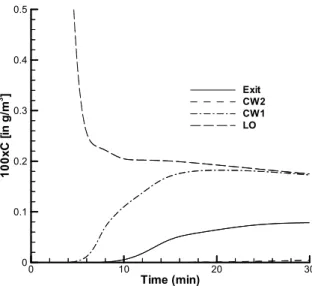
Qualitatively speaking, the general trends observed at CW1 (or HR=G), CW2

(or HR=F) and Exit (or HR=E) in Figs. 18 and 19 were similar. The concentration

level at CW2 is the smallest among the four HR locations examined. This is

because (1) the separation between LO and CW2 is the largest, and (2) the flow

velocity in the = (or LO=to=CW2) direction is very small (≈ −0.002 m s

) as

shown in earlier in Fig. 3. Furthermore, it can be seen from Figs. 18 and 19 that

the concentration level at Exit is the second smallest for this scenario because (1)

the separation between LO and Exit is smaller than that between LO and CW2,

and (2) the front door in Area I is open during the test.

%

; /

-

-*)

# $

/

!

)

% 3"

$

"!

: '

-

!

4

For this scenario, two additional personnel (CW1 and CW2) were involved. A

source of 0.1 g of BG spores in powder form was placed in a sealed envelope and

positioned at the location of the “Letter Opener” (LO) shown in Fig. 11. The

experimental personnel (LO, CW1 and CW2) were positioned initially about 0.5 m

in front of the tables (marked by Letter Opener, Co=worker 1 and Co=worker 2 in

Fig. 11). The HVAC system was turned on for about 15 minutes until the flow

reached a pseudo=steady state condition in the office, after which the BG spores

were released by opening the sealed envelope. The latter process was assumed to

take 10 s. Immediately after the BG spores were released from the opened envelope,

LO, CW1 and CW2 began to walk along the footprint pathway (trail) laid out on the

floor of the study area (shown in Fig. 20), finally exiting through the exit door. The

speed of walking of each person was about 1 ms

. It took approximately 12, 11 and

HVAC room (at = 5.5 s). The front door in Area I (close to the Co=worker 1

location in Fig. 11) was closed after the LO passed through it.

The rear door in Area I was left open during the simulation, in order to satisfy

“global mass conservation” in the study area (Areas I to IV plus the hallway).

Although the flow rates in cubic feet per minute (CFM) from all supply and return

ducts are provided by the experimental measurements and adjusted slightly to satisfy

area study in ducts return area study in ducts

supply

CFM

CFM

≠

∑

∑

(2)

mass conservation was not necessarily satisfied in Area I alone from the

measurements; i.e.

supply

CFM

CFM

≠

∑

∑

(3)

Equation (3) corresponds to the condition that prevailed when both front and

rear doors in Area I were closed. This caused numerical convergence problems in

our simulation. For this reason, the rear door was left opened throughout the

entire time period (30 minutes) for our simulation. This is the same time interval

for which the low=resolution (LR) slit samplers was activated in the experiment.

6 7 8 9 :

";;" +" " # = >" / # = >" 5

< >!

;%-%

: /

B C % *

0

& )1, -B

-B

#

&

Two cases were considered for Scenario 1. In Scenario 1a, the HVAC system

was turned on throughout the entire simulation period. In Scenario 1b, the HVAC

system was shut down by CW1 at time

= 5.5 s. Note that Scenario 1a is

to contaminate Areas IV, III and II through the doors in the hallway. In contrast,

as clearly seen in Fig. 23, the dispersion of the BG spores in the open office at

=1800 s (after the release) is still limited primarily to Area I when the HVAC

system was shut down soon after the opening of the sealed envelope. This

suggests that the advective mechanism, associated with a directed flow motion, is

more important than the turbulent diffusive mechanism for the dispersion of BG

spores for the current indoor conditions. Note that shutting down the HVAC

system not only reduced the mean flow, but also the level of turbulence in the

open office. Since the turbulent diffusion coefficient

Γ

∝

/

ε

( is the

turbulence kinetic energy and

ε

is the dissipation rate of turbulence kinetic

energy) is closely linked to the level of turbulence kinetic energy, shutting down

the HVAC system can be a very effective means for reducing the dispersion of

BG spores in the office, owing to the fact that both the advective and diffusive

mechanisms for dispersion are suppressed simultaneously.

If the HVAC system is turned on as in Scenario 1a, it is very important to

close both the front and rear doors to prevent the spread of BG spores from Area I

to the other areas in the open office, including the hallway. It is interesting to

compare Figs. 21 and 14 (Scenario 0) in order to see the effect of closing the front

door in Area I on the dispersion of BG spores. As expected, when the front door

is closed, the concentration contours in Fig. 21 show that the BG spores do not

even disperse to the end of the exit area after = 1800 s (30 min). Although we

were unable to simulate a scenario where both doors in Area I were closed due to

the fact that flow rates for both return and supply ducts were only measured when

both doors were opened, it is expected that most BG spores from the opened letter

will be “trapped” (and hence confined) inside Area I. Note that BG spores can

also enter the return ducts in Area I and, through the HVAC system (if it is turned

on) re=enter the hallway and Areas II to IV through the supply ducts. However,

this mechanism was not considered in the present numerical study

.

%

-

*

The bar plots of predicted concentration for Scenarios 1a and 1b are shown

in Figs. 22 and 24, respectively, which should be examined in conjunction

with Figs. 21 and 23. With the HVAC system turned on all the time (see Fig.

22), the concentration levels at SKC=2 to SKC=4 are larger than those with the

HVAC system turned off after = 5.5 s (see Fig. 24). In fact, the

concentration levels at SKC=3 to SKC=9 in Fig. 24 are less than 10

g/m

.

Fig. 24 can only be compared qualitatively with Fig. 25 (Trial 3 experiment)

because the units of concentration are different (g/m

compared to CFU per

Liter of Air). As in Fig. 17, SKC=1 (sampler on desk) and LO (or SKC=A)

sampler (worn by the letter opener) in Fig. 25 correspond to two different

samplers that are at slightly different locations in the vicinity of the desk (as

shown in Fig. 11). However, in our simulations, owing to the numerical

resolution, the SKC=1 and LO samplers in Fig. 24 (simulation) represent

exactly the same location, both of which are taken at the center of the desk

(table). One encouraging result here is that

/

≈ O(10

) for both the

experimental measurements and the numerical simulation. It can be seen from

Fig. 25 that the concentration levels at SKC=2 and SKC=3 are comparable,

which contradicts the numerical predictions shown in Fig. 24 (where the

concentration level at SKC=3 is seen to be much smaller than that at SKC=2).

Since the HVAC system is turned off most of time in the experiment and in

the Scenario 1b simulation, it is quite unlikely that the concentration level at

SKC=2 (which is nearby LO) can be comparable to that at SKC=3. There are

two reasons that could cause this “anomaly”: namely, (1) as LO passes close

to SKC=3, it may have contaminated this sampler, leading to an increase in

the observed concentration; or, (2) the air flow leakage through the building

shell may be a cause for the above=mentioned difference.

%

'

-

*

-

%=

A-

$

6

%

-

*

-2 - /

8 5 5 !

8 9::

:

!

%

4 '

-

*

-

%=

%

5 '

-

-

# $

/

!

- 0 $

)

A-

$

)

4

In Scenario 2, CW1 and CW2 leave Area I and exit through the exit door

immediately after the BG spores were released from the opened letter. The LO

remains still for 5 min before he too exits the test area, following the same

footprint pathway as shown in Fig. 20. We only have flow rate measurements for

the supply and return ducts when all the doors in Area I were opened as in the SF

experiment. However, we found that numerical convergence problems occurred in

our simulations if all doors were closed, as mentioned earlier in the discussion

following Eq. (3). Consequently, in the current simulation, the front door was

closed only after the LO left the test area. The rear door of Area I was left opened

throughout the test.

Figures 26 to 28 show contours of predicted concentration at = 8.75 s (BG

spores were still being released, while the LO remains stationary after opening the

envelope), at = 310.75 s (the LO is about to exit through the exit area), and at =

1800 s (30 min). Since CW1 and CW2 leave the test area at a walking speed of

about 1 m s

, which is much faster than the rate at which BG spores are

dispersing near the LO, their motions practically cause no disturbance to the

dispersion of BG spores. In this simulation, both doors in Area I remained open

for the first 300 s. As a result, it is seen from Fig. 27 ( > 300 s) that the BG

spores have already dispersed into the hallway near the exit area after the front

door was closed. At the end of the simulation ( = 1800 s) shown in Fig. 28, a

portion of the BG spores which were excluded from Area I in Fig. 27, have

already spread in both directions from near the front door towards the exit area (to

the right) and towards Areas II and III (to the left). Area IV is the only area for

which the BG spores have not as yet dispersed into.

7

SKC=9) the concentration was below 10

g/m

, with the exception of the locations at

SKC=1 (or LO) and SKC=2 (or CW1). It is informative to compare Fig. 24 (in which

the front door was closed after = 5.5 s) and Fig. 29 (in which the front door was

closed after = 305.5 s). For both cases, the HVAC system was turned off after = 5.5

s. The concentration levels at LO and SKC=2 in both figures are very comparable,

although concentration at SKC=2 in Fig. 24 is slightly smaller than that in Fig. 29.

This might be due to the presence of the LO at the desk (during the first 5 min after

the letter was opened) who may have obstructed (or, constrained) the spread of BG

spores in the case of Fig. 29 (cf. Fig. 26).

%

-

*

-89 75

1$

%

)

%

7 -

*

8

%

9 -

*

-8 9::

:

!

1$

%

)

%

; '

-

*

-

%=

A-

$

)

The experimental data (Trial 3) for this scenario, shown in Fig. 30 in CFU per

Liter of Air instead of in g/m

, is quite different from the numerical predictions,

especially in terms of

/

. The predicted

/

is O(10

), whereas the

LO

/

from the experimental measurements is O(10). It should be noted here

that

/

≈

O(10

) in Scenario 1 for both the numerical predictions and the

9

(see Fig. 30) are O(10) larger than those shown in Fig. 25 (Scenario 1). Also, the

concentration level at the LO shown in Fig. 30 is O(10) smaller than that shown

in Fig. 25. Since the HVAC system was turned off in both experiments, it is

possible that this discrepancy can be attributed to the air flow leakage through the

cracks and crevices in the building shell, particularly in Scenario 2. Another

contributing factor to the discrepancy might be an experimental anomaly. This is

illustrated in Fig. 31, in which

/

≈

O(10

2

) for Trial 5 and

/

≈

O(10) for Trial 3 (essentially an “identical” replication) as seen in Fig. 30,

suggesting that the variability in measurements even on nominally identical

replications is large.

%

: '

-

-

# $

/

!

- 0 $

)

A-

$

)

%

'

-

-

# $

/

5!

:

In this experiment, CW1 and CW2 exit the study area immediately after the LO

informs them that he has opened a letter containing the BG spores. Both front and rear

doors are closed as soon as CW1 and CW2 leave Area I. However, it is still possible

that a small portion of BG spores deposit on CW1 and disperse into the study area

outside Area I as CW1 walks along the prescribed path shown in Fig. 20. This

hypothesis is supported by the reasonably high concentration levels measured at

locations of SKC=4 to SKC=9, which are outside Area I. In contrast, the predicted

concentration levels shown in Fig. 29 are less than 10

g/m

at SKC=4 to SKC=9,

because deposition and re=suspension are not considered in the numerical simulation.

5 -

"

In the present study, two experiments, namely SF6 and BG spore release

experiments were simulated using CFD. In the SF6 release experiment,

ventilation measurements in terms of volumetric flow rate were conducted, and

the time histories of concentration in ppm at 6 sampler locations were available.

This, in principle, could be predicted by CFD simulations if the laboratory

environment (study area) is well controlled (viz., if there are no air flow leakages

in the study area). The BG release experiments, however, were much more

challenging to simulate because the concentration units used in the experimental

measurements (e.g., CFU per Liter of Air or ACPLA) cannot be related

unambiguously to the mass of BG spores released from the opened letter. More

specifically, the number of spores in the sealed envelope in colony forming units

(CFU) was unknown, and the actual number of BG spores released when the

letter was opened was also unknown. Furthermore, the effect of deposition and re=

suspension of BG spores in the indoor environment was not considered in our

simulations. Therefore, we can only make qualitative, rather than quantitative

comparisons, between the numerical predictions and the experimental

measurements of BG concentration because the exact conversion between CFU

per Liter of Air, ACPLA and g/m

is not known. As well, the precise amount of

BG spores released from the opened letter was not known.

In the case of the BG release experiments, three different scenarios were

simulated. Two of these scenarios involved experimental personnel leaving the study

area. In order to numerically model the effects of one or more persons moving

through the study area and exiting the office, a first=order Immersed Boundary

Method (IBM) was implemented in the CFD flow solver STREAM. Overall, CFD is

able to generate very realistic flow and concentration fields in the indoor environment,

even with the HVAC system turned off at an early stage in the experiment and with

people moving through the study area. The detailed simulations permitted the

following conclusions to be drawn and recommendations to be made.

For the SF

experiment, we believed that the flow rate measurements for the

supply and return ducts are accurate. Therefore, it is hypothesized that the

discrepancy between the numerical predictions and experimental measurements of

concentration were mainly caused by (1) air flow leakage from cracks and crevices

in the building envelope and, (2) dispersion of SF

in the HVAC system. Both these

environment that has been certified to be airtight. To address the second cause for

the discrepancy, the CFD model used here for the simulation of flow and dispersion

in an open office can be coupled with a zonal model (such as COMIS or

CONTAM), to simulate the flow and dispersion in the HVAC system. This

CFD/zonal=model coupling should improve the numerical predictions for the SF

experiment and Scenario 0 (Baseline Case) for the BG release experiment, in which

the HVAC system was turned on throughout the entire experiment.

The flow rate measurements for the supply and return ducts obtained for the SF

experiments were used in our simulations of the BG spore experiments. This is

questionable for Scenarios 1 and 2, in which personnel are moving in the study area

and the doors in Area I were closed. In both scenarios, unsteady CFD simulations

were performed. Since both front and rear doors in Area I were closed as the various

personnel exited the study area, the ventilation measurements in Area I alone will

need to be modified as suggested by Eq. (3), the latter of which is based on the

argument of global mass conservation in Area I. In theory,

flow rate

measurements for the supply and return ducts should be made available and used as

boundary conditions to perform the CFD simulations. As a minimum requirement to

simulate the BG experiment, volumetric flow rates for the supply and return ducts

should be measured for the following scenarios: (a) with only the two middle doors in

Area I closed, and (b) with all four doors in Area I closed. To address the effects of

BG spore deposition on the predictions, it is recommended that the present unsteady

RANS approach be combined with an eddy interaction model (EIM, or random walk

model) for modeling aerosol dispersion and deposition. EIM is based on a Lagrangian

stochastic approach, in which individual particles are allowed to interact successively

with discrete eddies (see, e.g., [21, 22]).

Finally, it should be emphasized here that the advantages of utilization of CFD

modeling for assessment and design of mitigation strategies and protocols for

defence against anthrax=tainted letters are obvious: (1) substantial reduction of

lead times and costs of new designs involving other office configurations; (2)

ability to study scenarios where controlled experiments are difficult or impossible

to perform; and, (3) practically unlimited level of detail of results such as the flow

field in the indoor environment and the concentration field of the dispersing BG

spores (or, other contaminants) that are released into this flow field.

"

1.

de

Armond,

P.

(2002).

The

anthrax

letters.

Albion

Monitor,

http://www.monitor.net/monitor/0208a/anthrax.html.

2.

Kournikakis, B.; Armour, S.J.; Boulet, C.A.; Spence, M.; and Parsons, B.

(2001). Risk assessment of anthrax threat letters.

!

"

#

!!

, DRES TR=2001=048.

3.

Duncan, S.; Kournikakis, B.; and Ho, J. (2009). Pulmonary deposition of

aerosolized

(BG) in an awake, unrestrained swine model

due to exposure from a simulated anthrax letter incident.

$

, 21(2), 141–152

4.

Kournikakis, B.; Walker, M.; Ho, J.; and Duncan, S. (2009). Statistical

analysis of bacterial spore aerosols created by opening a spore containing

5.

Kournikakis, B.; Ho, J.; and Duncan, S. (2010). Anthrax letters: personal

exposure, building contamination and effectiveness of immediate mitigation

measures.

%

! '

#

, 7(2), 71=79.

6.

Price, P.N.; Sohn, M.D.; Lacommare, K.S.H.; and Mcwilliams, J.A. (2009).

Framework for evaluating anthrax risk in buildings.

#

, 43(6), 1783–1787.

7.

Reshetin, V.P.; and Regens, D. (2004). Evaluation of malignant anthrax spore

dispersion in high=rise buildings.

%

! #

(

, 77(6), 1155–1166.

8.

Lien, F.S.; and Leschziner, M.A. (1994). A general non=orthogonal

collocated finite volume algorithm for turbulent flow at all speeds

incorporating

second=moment

closure,

Part

1:

Computational

implementation.

)

&

)

#

,

114 (1=2), 123=148.

9.

Lien, F.S.; and Leschziner, M.A. (1994). Upstream monotonic interpolation

for scalar transport with application in complex turbulent flows.

$

%

!

*

)

+

, 19(6), 527=548.

10. Leonard, B.P. (1979). A stable and accurate convection modelling procedure

based on quadratic upstream interpolation.

)

&

)

#

, 19(1), 59=98.

11. Patankar, S.V. (1980).

*

!

!

! ,

. Hemisphere

Publishing Corporation.

12. Stone, H.L. (1968). Iterative solution of implicit approximations of

multidimensional partial differential equations.

$&) %

*

&

, 5(3), 530–558.

13. Rhie, C.M.; and Chow, W.L. (1983). A numerical study of the turbulent flow

past an isolated airfoil with trailing edge separation.

&$&& %

, 21(11),

1525=1532.

14. Aftosmis, M.J.; Berger, M.J.; and Melton, J.E. (1998). Robust and efficient

cartesian mesh generation for component based geometry.

&$&& %

,

36(6), 952=960.

15. Peskin, C.S. (1977). Numerical analysis of blood flow in the heart,

%

!

(

, 25(3), 220=252.

16. Tseng, Y.H.; and Ferziger, J.H. (2003). A ghost=cell immersed boundary

method for flow in complex geometry.

%

!

(

,

192(2), 593=623.

17. McCleery, R.E. (2006), National institute for occupational safety and health

(NIOSH),

.

18. COMIS. http://epb.lbl.gov/comis/.

19. CONTAM. http://www.bfrl.nist.gov/IAQanalysis/index.htm.

20. Hsieh, K.J.; Lien F.S.; and Yee, E. (2007). Numerical modelling of scalar

dispersion in an urban canopy.

%

! -

#

. $

&

, 95(12), 1611=1636.

21. Graham, D.I.; and James, P.W. (1996). Turbulent dispersion of particles

using eddy interaction models.

$

%

! )

+ ,

,

22(1), 157=175.

22. Wang, L.P.; and Stock, D.E. (1992). Stochastic trajectory models for

turbulent diffusion: Monte Carlo process versus Markov chains,

&