Representative Sinusoids for Hepatic
Four-Scale Pharmacokinetics Simulations
Lars Ole Schwen1
*, Arne Schenk2,3, Clemens Kreutz4, Jens Timmer4,5, María Matilde Bartolomé Rodríguez6, Lars Kuepfer2,7, Tobias Preusser1,8
1Fraunhofer MEVIS, Bremen, Germany,2Computational Systems Biology, Bayer Technology Services, Leverkusen, Germany,3Aachen Institute for Advanced Study in Computational Engineering Sciences, RWTH Aachen University, Aachen, Germany,4Freiburg Center for Data Analysis and Modeling (FDM), Institute of Physics, University of Freiburg, Freiburg, Germany,5BIOSS Centre for Biological Signalling Studies, University of Freiburg, Freiburg, Germany,6Clinic for Internal Medicine II/Molecular Biology, University of Freiburg Medical Center, Freiburg, Germany,7Institute of Applied Microbiology, RWTH Aachen University, Aachen, Germany,8Jacobs University, Bremen, Germany
Abstract
The mammalian liver plays a key role for metabolism and detoxification of xenobiotics in the body. The corresponding biochemical processes are typically subject to spatial variations at different length scales. Zonal enzyme expression along sinusoids leads to zonated metabo-lization already in the healthy state. Pathological states of the liver may involve liver cells affected in a zonated manner or heterogeneously across the whole organ. This spatial het-erogeneity, however, cannot be described by most computational models which usually consider the liver as a homogeneous, well-stirred organ.
The goal of this article is to present a methodology to extend whole-body pharmacokinet-ics models by a detailed liver model, combining different modeling approaches from the lit-erature. This approach results in an integrated four-scale model, from single cells via sinusoids and the organ to the whole organism, capable of mechanistically representing metabolization inhomogeneity in livers at different spatial scales. Moreover, the model shows circulatory mixing effects due to a delayed recirculation through the surrounding organism.
To show that this approach is generally applicable for different physiological processes, we show three applications as proofs of concept, covering a range of species, compounds, and diseased states: clearance of midazolam in steatotic human livers, clearance of caf-feine in mouse livers regenerating from necrosis, and a parameter study on the impact of dif-ferent cell entities on insulin uptake in mouse livers.
The examples illustrate how variations only discernible at the local scale influence sub-stance distribution in the plasma at the whole-body level. In particular, our results show that simultaneously considering variations at all relevant spatial scales may be necessary to understand their impact on observations at the organism scale.
OPEN ACCESS
Citation:Schwen LO, Schenk A, Kreutz C, Timmer J, Bartolomé Rodríguez MM, Kuepfer L, et al. (2015) Representative Sinusoids for Hepatic Four-Scale Pharmacokinetics Simulations. PLoS ONE 10(7): e0133653. doi:10.1371/journal.pone.0133653
Editor:Manlio Vinciguerra, University College London, UNITED KINGDOM
Received:April 17, 2015
Accepted:June 29, 2015
Published:July 29, 2015
Copyright:© 2015 Schwen et al. This is an open access article distributed under the terms of the
Creative Commons Attribution License, which permits unrestricted use, distribution, and reproduction in any medium, provided the original author and source are credited.
Data Availability Statement:All relevant data not taken from cited literature are within the paper and its Supporting Information files.
Introduction
The liver plays a pivotal role for metabolization and detoxification in the mammalian body. The connection between the whole organism and the liver is mainly given by blood flow: blood is supplied to the liver via two vascular systems, portal vein (PV) and hepatic artery (HA), blood is drained via the hepatic vein (HV). The PV and HA provide approximately 75% and 25% of the inflow, respectively [1]. Besides the blood flow, additional exchange between organ and organism is given by bile [1] and lymph [2] flow.
Clearance contributions of different organs are typically analyzed by pharmacokinetics (PK) models [3–5]. In particular, specific models for liver clearance were developed [3,6]. One major challenge for PK simulations, in particular for relevant diseased states, is the presence of spatial inhomogeneity and multiple scales in time and space that need to be accounted for appropriately. The most prominent spatial scales in the liver are:
1. individual hepatocytes performing most of the metabolization of diameter 20 to 40μm [1] in humans, 23.3 ± 3.1μm in mice [7];
2. sinusoids and space of Disse along which the blood gets in contact with the hepatocytes;
3. lobuli consisting of multiple sinusoids draining to the same central vein. Lobuli have a diameter of 1 to 1.3 mm and a depth of 1.5 to 2 mm in humans [1]. Their radius is 284.3 ± 56.9μm in mice [7]. The radius of a lobulus is thus about 19 hepatocyte diameters in humans and 12 in mice;
4. the liver and its lobes, organized in many lobuli, supplied and drained by the main major branchings of the hepatic vascular structures. The total liver volume is about 1.5 l in humans [1] and approximately 1.1 ml in mice [8]. Human livers are classically divided in two lobes or eight segments [9], but there is no consensus in the literature on the subdivision and its terminology, neither for mice [10] nor for humans [11].
Two of these length scales of inhomogeneity are most relevant for metabolic processes. On the sinusoidal length scale, effects occurring in specific regions along sinusoids are denoted by zonation[12,13]. In case we do not refer to a small number of zones, we will denote this by sinusoid-scale heterogeneity. Furthermore, metabolic effects can differ between lobuli found at different locations in or across lobes. We will denote the latter byorgan-scale heterogeneity. Generally, three main reasons for inhomogeneous metabolization can be distinguished:(a) Theperiportalhepatocytes, those near the inflow to the sinusoid, experience a higher concen-tration of a compound being metabolized than thepericentralhepatocytes, those near the out-flow. This may lead to concentration gradients even if the cells themselves do not differ in terms of their metabolic capability.(b)Different gene expression or enzyme levels depending on the location, either along sinusoids or throughout the organ, may additionally lead to spatial differences in the metabolic capability.(c)Pathological states can furthermore affect the meta-bolic capability, see the examples inFig 1showing steatosis patterns at different length scales.
The goal of this article is to introduce a generic simulation framework capable of dealing with both types of spatial inhomogeneity, i.e., sinusoid-scale as well as organ-scale heterogene-ity. It is intended to mechanistically model the underlying effects and allow predictions in the case of pathophysiological changes. The key building block of the multiscale model presented here corresponds to the sinusoidal scale and is denoted byrepresentative sinusoids. Each such representative sinusoid contains a spatial pattern of metabolization parameters and stands for one region of the liver exhibiting essentially this same parameter pattern. An organ-scale het-erogeneity can thus be represented in the model by taking into account multiple representative sinusoids in parallel.
role in the study design, data collection and analysis, decision to publish, or preparation of the manuscript. The specific roles of these authors are articulated in the“author contributions”section.
Review of Related Pharmacokinetics Simulation Techniques
Physiologically based pharmacokinetic (PBPK) modeling mechanistically represents whole-body physiology at an organism level. In contrast to rather generic compartments in classical PK modeling, PBPK models consider organs explicitly, allowing amongst others for the simula-tion of time-concentrasimula-tion profiles in specific tissues. PBPK models may comprise systems of ordinary differential equations (ODE system) in several hundreds of variables and an equally high number of model parameters. The number of independent model parameters, however, is significantly smaller, i.e., around 5 to 10, due to the large degree of prior information contained in the PBPK software tools. For example, physiological model parameters such as organ vol-umes or organ surface areas are usually available from integrated, species-specific data collec-tions [15]. To calculate the remaining model parameters, only physicochemical properties of a compound, such as lipophilicity or molecular weight, need to be provided by the user to parametrize the PBPK model [15].
For PBPK model building itself, it is essential to have prior information about the governing physiological processes underlying absorption, distribution, metabolization, and excretion. The physicochemical properties of a compound are used to estimate, e.g., tissue permeation by passive distribution. Active processes such as enzyme-catalyzed metabolization or transporter-mediated uptake or secretion may also be mechanistically considered at the organism level by using tissue-specific gene expression profiles [16]. The degree of biological knowledge included in PBPK models hence ranges from tissue-specific gene expression profiles at the cellular scale to anthropometric parameters at the organism level. For model establishment and model validation, time-concentration profiles are required. PBPK is nowadays routinely used in phar-maceutical development specifically supporting the various stages in the research and develop-ment process for example for risk assessdevelop-ment [17], pediatric scaling [18] and cross-species extrapolation [19].
Sinusoid-Scale and Organ-Scale Homogeneous Models. Models without spatial resolu-tion are frequently used if a zonaresolu-tion of metabolic capability is unknown or does not play a role, e.g., if a compound is not metabolized at all by a given organ. Such models are structured as compartmental models without spatial resolution of organs [20,21], or combine multiple organs in one generic compartment [22,23], and therefore assume that a description corre-sponding to awell-stirredsetting is appropriate.
Fig 1. Steatosis Inhomogeneity.Theleftimage shows a histological image of a human liver with selected portal fields and central veins marked asand⊗, respectively. Therightimage shows a histological whole-slide scan of a steatotic mouse liver and a zoom to one lobe. Macrovesicular steatosis, i.e., lipid
accumulations of diameter larger than hepatocyte nuclei, was quantified in all cases using an image analysis method based on [14] and visualized as an overlay to the histological images, using a color map from violet to yellow indicating low to high steatosis. The left example shows a pericentrally zonated state of steatosis. The right example shows both organ-scale and lobe-scale heterogeneity in the steatosis distribution in addition to a periportal zonation not clearly visible at this magnification. The human image data is by Serene Lee and Wolfgang Thasler, Department of General, Visceral, Transplantation, Vascular and Thoracic Surgery Ludwig Maximilians University Munich Medical Center; the mouse image data is by Uta Dahmen, Department of General, Visceral and Vascular Surgery, University Hospital Jena; the analysis overlay was provided by André Homeyer, Fraunhofer MEVIS, Bremen.
Sinusoid-Scale Heterogeneous, Organ-Scale Homogeneous Models. Any metabolic pro-cess along a sinusoid introduces a spatial concentration gradient, particularly prominent for compounds subject to significant first-pass elimination [24]. Additionally, metabolic capabili-ties of neighboring cells along a sinusoid can be distributed inhomogeneously along the sinu-soid. This can be due to gene/enzyme expression [25,26] or zonal presence of other cell types [25]. Examples in this category are carbohydrate metabolism [25], ammonia detoxification [27], and cytochrome metabolism for which two cases are considered in this article. Zonated metabolization can also be caused by pathological conditions appearing zonally, two examples are considered in this article: necrosis after CCl4intoxication [28] and different states of
steato-sis [29]. Processes involving sinusoid-scale heterogeneity can be modeled by using sequential well-stirred compartments [4,5,30,31] for the liver. Other approaches build a zonation into lobule-scale models containing multiple sinusoids and their surrounding cells (cf. [32] model-ing lobular perfusion and [33,34] modeling lobular perfusion and PK) or into multiphase con-tinuum models (cf. [35,36] modeling lobular perfusion and [37] modeling lobular perfusion and PK).
Organ-Scale Heterogeneity. Metabolization may additionally be heterogeneous at the organ scale, due to differences between sinusoids at different position in the organ. This is mainly due to pathological conditions varying at this length scale. Examples include steatosis [29,38], fibrosis due to nonalcoholic steatohepatitis [39] or in case of hepatitis C [40], cirrhosis [41], granuloma [41], and carcinoma [42,43]. Another reason can be heterogeneous concen-tration sources, e.g., due to intrahepatic injection via catheters [44] or targeted drug delivery [45]. Appropriate modeling techniques for the case of organ-scale heterogeneity without addi-tional zonation are given by multiple parallel well-stirred compartments per organ [20,31,46,
47]. Organ-scale porous-medium-based multiphase continuum models [8] can be used as well. These are, however, of limited practical applicability if also a sinusoid-scale heterogeneity is present as they require high spatial resolution in this case. A combination of multiple parallel and sequential well-stirred compartments [31] per organ can be used in case of organ-scale het-erogeneity combined with zonation. Also a parallel use of recent cell-based [34] or multiphase porous-medium-based [37] lobule-scale models is conceivable.
In any case, the structure of the model should be chosen depending on what is relevant for the application being considered. It should sufficiently detailed to capture relevant effects, but no more detailed to avoid unnecessary need for parameters and potentially error-prone model assumptions, and to keep computational workload at bay. This in particular implies that it can be useful to consider different degree of detail for representing different organs or organ groups [23].
We point out that this section not meant to be an exhaustive literature review of PK model-ing. For more detailed reviews, we refer to [4,5,31].
Introducing a Multiscale Simulation Framework Based on
Representative Sinusoids
scales and represents the blood flow as a process in its own right. For a more detailed overview on fluid transport systems in different organs, we refer to [49]. We here use mathematical advection and reaction equations to model blood flow through blood vessels, trans-vascular compound exchange, and chemical kinetics. A more detailed description of the biological pro-cesses we model here is given in [50].
The approach presented here is also an extension of our previous work [8] in which the organ is resolved at a single scale as a porous medium. We here consider two spatial scales for the organ tissue: representative sinusoids and individual cells. One such representative sinusoid can capture sinusoid-scale heterogeneity at the appropriate physiological length scale, while different representative sinusoids can be assigned to different locations throughout the organ in case of organ-scale heterogeneity. This approach can be embedded in a simulation frame-work using multiple spatial scales [51]. At the cellular scale, effective behavior from the finer intracellular scale is integrated in the model via the parameters in the exchange/metabolization ODE system. For the coarser organism scale, our technique can act as a‘liver module’. The organism scale is currently implemented by an ODE system representing recirculation through the body allowing for metabolization also in other organs, albeit not at the level of detail as in the liver. Other multiscale PK modeling approaches include, e.g., the integration of intracellular signaling [15] or metabolic networks [52] into the cell representation. We refer to [53,54] for two overviews on multiscale PK modeling approaches and to [55] for approaches of integrating intestinal models and an effective description of the body scale.
Comparison to Related Approaches. Our approach has the same goal of multiscale liver modeling as the two recent models [37] dealing with glucose metabolism and [34] considering ammonia detoxification. These approaches differ on a technical level and thus have slightly dif-ferent foci. The model in [37] considers homogenized multiphase flow in a 2D model lobulus and determines flow velocities as part of the simulation. The model in [34] uses a 3D slice as part of a lobulus with sinusoids and individual hepatocytes. In addition to performing metabo-lization, the hepatocytes in [34] can grow, divide, and migrate, which allows modeling regener-ation in more detail. Consequently, these approaches provide more detail at the lobular level than the simplified 1D sinusoids used in our approach. This, however, implies a higher compu-tational workload for simulation when using more detailed lobular models. While it is certainly possible to extend these to including organ-scale heterogeneity, i.e., many different lobule mod-els with different parameters, efficiency then becomes a challenge.
On the cellular level, [37] considers model of glucose metabolism obtained by model reduc-tion from a detailed kinetic model, whereas [34] and our approach use equations of a given structure with parameters representing biochemical properties and/or parameters fitted to experimental data. It should, however, be possible to use any of these models or also more detailed intracellular models in either approach. Similarly, the extrahepatic models differ, but could in principle be exchanged between the different approaches. In [37], liver inflow concen-tration profiles are used as model input, corresponding to an isolated perfused liver [56,57] model. In [34], a three-compartment body-scale recirculation model is used. We consider an isolated perfused liver in one of the example applications presented below, the other two appli-cations involve a multi-compartment body-scale recirculation model representing each indi-vidual organ in the respective human or murine body. Given appropriate model parameters, this permits a more detailed investigation of the role of the different organs for the compound being investigated. Detailed recirculation models increase the computational workload of the simulation. This is not a major challenge for our purpose as the additional workload for the extrahepatic model does not scale with the degree of hepatic organ-scale heterogeneity.
organ and sinusoids to the cells, and back, is provided via the blood flow. Bile flow and lymph flow, such as considered in [36], are not part of our model as the flowing volumes are negligible compared to the blood flow.
Recirculation through the organism(body scale)outside the liver as well as possible accumu-lation and metabolization in other organs are considered in effective form and in particular not at the same degree of detail as for the liver. For this purpose, an ODE system describing the whole-body PBPK model for the substance under consideration is used. These ODE systems are solved numerically using standard backwards differentiation formula (BDF) techniques [58]. The recirculation takes into account the temporal delay of the blood flowing through the organism.
On theorgan scale, the heterogeneity of metabolization or pathology parameters determines the number and size of regions of different parameter values needed. To represent the connec-tion between the organism and the sinusoids, the hepatic vascular systems distributing the blood throughout the organ are taken into account. The concentrations flowing from the body to the liver are hereby transported to each representative sinusoid with a given temporal delay. The outputs of the representative sinusoids with the respective temporal delays are summed up and form the concentrations flowing from the liver back to the body. In both vascular systems, only advection is considered. In particular, exchange between red blood cells and plasma and any metabolization processes are omitted in the blood vessels. As velocities are constant along each edge and over time, an advection simulation as in [8] is not necessary here and it is suffi-cient to consider appropriate delay times for different paths through the vascular system. If the actual geometrical configuration of regions of the same sinusoid-scale parameter patterns does not need to be reflected in the simulation, in particular if no exact temporal correspondence between different representative sinusoids is necessary, the vascular systems do not need to be considered for the simulation. In this case, only the relative contribution of each representative sinusoid for the whole organ and possibly the respective temporal flow delay are needed. Let us, however, point out that the simulation results can still be mapped to the actual geometric position for interpretation or visualization if needed. Depending on the organ-scale parameter heterogeneity, the liver model contains several representative sinusoids.
The representative sinusoids(sinusoidal scale)are used to model the actual exchange of compounds between the blood and the liver cells as well as the metabolization in the cells. For
Fig 2. Model Overview.The figure shows the four spatial scales present in our multiscale pharmacokinetics simulation framework. The connection between the scales is given by the blood flow, indicated by arrows. The‘representative sinusoids’are the central building blocks in our framework. For each of these, we solve an advection-reaction problem. (HA: hepatic artery; HV: hepatic vein; PV: portal vein.)
this purpose, the sinusoid is viewed as consisting of four subspaces: red blood cells (RBC), plasma, interstitium, and cells. The interstitium mainly represents the physiological space of Disse, the cells primarily refer to the hepatocytes. This means that the actual sinusoid only cor-responds to the red blood cells and the plasma. However, to simplify terminology, we view the adjacent interstitium and cells as part of the representative sinusoid. The compound under consideration is exchanged between the subspaces and metabolized in the cellular subspace. This structure is chosen in analogy to the liver subcompartments in PBPK models [59] and was previously used in [8]. In addition, the compound concentration is subject to blood flow with constant flow velocity in the RBC and plasma subspaces. Exchange and metabolization at thecellular scaleare described by cell-specific ODE systems with potentially different parame-ters to reflect sinusoid-scale heterogeneous patterns. Blood flow is represented by a one-dimen-sional advection PDE, so that we obtain an advection-reaction problem for each representative sinusoid. We will apply a combination of a Eulerian–Lagrangian Localized Adjoint Method (ELLAM) [60] and Runge–Kutta–Fehlberg 4th/5th order [61] time stepping to solve these numerically. Our approach considers sinusoids at their correct physiological length scale, even though one sinusoid in the model represents larger regions in the liver. In contrast to models using a series of well-stirred compartments without delay [20,30,47], modeling the blood flow by advection inherently represents the physiological delay of flowing through a sinusoid with a given velocity. This provides more accurate temporal resolution at sub-second or second time scales, which is a relevant time scale for some applications, e.g., [62].
Outline
The present article is further organized as follows: We introduce our multiscale model starting from a PBPK model; describe the processes included at additional scales; how this is modeled, discretized, and implemented; and how two pathological cases are modeled. Three example applications illustrate that this simulation approach is applicable to a broad range of pharma-cokinetic and physiological questions. We consider(a)the clearance of midazolam in human livers affected by steatosis, a zonated process subject to a zonated and organ-scale heteroge-neous pathological condition,(b)the clearance of caffeine in regenerating mouse livers, a zonated process subject to a zonated pathological condition changing over time, and(c)a parameter study on different cell entities performing insulin uptake in mouse livers, investigat-ing different spatial patterns of the cell entities along a sinvestigat-ingle sinusoid. Finally, we discuss the present limitations and further perspectives.
Methods
In this section, we describe the components of our multiscale model, i.e., the building blocks at the different spatial scales. We start addressing the body and cellular scale where we use and extend an existing PBPK model using well-stirred compartments for each organ. Next, geome-try and flow on the organ scale is considered before we address the sinusoidal scale, introducing the key component of our approach. The interaction of the building blocks and necessary translations for models of different dimensionality are presented in. Finally, we introduce two model perturbations representing diseased states of the liver. An overview of the models and their dimensionality for the processes at the different spatial scales is given inTable 1. Specific compounds and their PBPK models for the cellular scale are addressed later in the results section.
respective positions, we briefly address how the methods can be extended to multiple com-pounds, in particular when taking into account the formation of metabolites.
Model Building Blocks at the Body and Cellular Scales
The starting point for our multiscale model is a whole-body PBPK model implemented in PK-Sim [59] where organs are represented as well-stirred compartments, i.e., zero dimensional. This model without its liver component will be adapted for simulating recirculation through the organism, the liver component will be used as the basis of our refined liver model. Let us point out that the body-scale recirculation can also be omitted if an isolated perfused liver [56,
57] is considered.
Body-Scale Recirculation Model. The body-scale PBPK model [59] describes the blood flow between the organs, and thus the transport of a compound through the body, as well as the exchange of compounds between subcompartments of the organs and the metabolization. These processes are described by a non-linear ODE system in several hundred variables.
On the body scale, it is necessary to consider a temporal delay of the recirculation. In certain cases, more than one initial pass of an injected compound can be observed experimentally, see, e.g., [62] for measurements of antipyrine in dogs or [63] for an MRI contrast agent in humans. An ODE model not taking into account the temporal delay of the blood flow between and through the different organs is generally not capable of reproducing second and further passes. This is not an issue for observations on the time scale of hours or days, but should not be ignored when simulating processes on the time scale of seconds to minutes.
In our model, we integrate this temporal delay of the recirculation as a delayτbodyfor
blood flowing between the lung and the systemic arterial blood pool, the latter supplying all organs in the model. This delay thus affects the compound mass flows in the red blood cells and the plasma from the lung to the arterial blood pool. This location in the PBPK model was chosen because all recirculating blood passes through the lung. The body delayτbodywas
computed as follows: First, letτrec totaldenote the total recirculation time through the body
obtained as total blood volume in the organism divided by the blood flow rate through the lung [59], resulting in
trec total ¼ 54:8s in humans;
19:7s in mice: ð1Þ
(
We refer to the results section below for a discussion about how these values differ from the measurements in [63]. The recirculation time [64] and time between peaks can be expected to differ due to intra-organ retention of compounds. From the valuesτrec total, two transit times
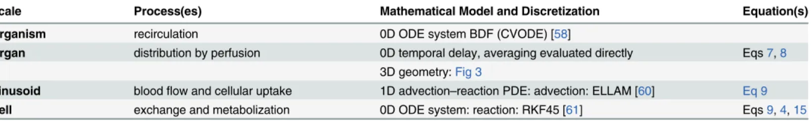
Table 1. Processes and Numerical Techniques.The table gives an overview of the processes being modeled and the numerical techniques applied in each of the model building blocks for the distinct spatial scales, cf.Fig 2. The overall model requires an integration of submodels of different dimensionality: from 0D, referring to models where spatial effects are not explicitly considered, via 1D sinusoids to a 3D organ. Round brackets in the table refer to equations in this article, square brackets to literature.
Scale Process(es) Mathematical Model and Discretization Equation(s)
Organism recirculation 0D ODE system BDF (CVODE) [58]
Organ distribution by perfusion 0D temporal delay, averaging evaluated directly Eqs7,8
3D geometry:Fig 3
Sinusoid bloodflow and cellular uptake 1D advection–reaction PDE: advection: ELLAM [60] Eq 9
Cell exchange and metabolization 0D ODE system: reaction: RKF45 [61] Eqs9,4,15
explained below are subtracted to obtainτbody, namely the sinusoidal transit time, seeEq 6, and
the transit time for the hepatic vascular systems, if present in the model, see Eqs7and8. Clearly, this recirculation delay model is not mechanistic, highly simplified, and does not take into account flow delays within or between the individual organs. In a similar manner as for the whole body, we could use specific transit times for each organ, namely dividing the respective blood volume by the respective flow rate. This would make the implementation more technical and increase computational costs for the simulations, but it is not clear to what extent the overall model accuracy would benefit. As this article focuses on the liver, we will leave the recirculation delay model open for future model refinement.
The ODE systems describing recirculation turned out to be very stiff. For solving stiff ODE systems, various numerical methods are available [65,66]. Based on a brief performance evalu-ation, we chose a scheme using a BDF scheme available as part of CVODE solvers [58], based on [67], in the SUNDIALS library [68] to solve the recirculation ODE systems. This part of the simulation turned out not to be very time critical, so passing values between our simulation and an external ODE solver is no performance bottleneck.
Physiologically Based Pharmacokinetics Models Used for the Cellular Scale. The recir-culation ODE systems are expressed in terms of the molar amounts of the compound in differ-ent organs. For introducing spatial resolution, we use molar concdiffer-entrations in the other building blocks of our multiscale model and as the interface to the recirculation model. Throughout this article, concentration is always meant as molar concentration in units mM = mol m−3, unless stated otherwise.
To describe the connection between organism and organ, we generally distinguish between concentrationscfflowing in the blood and concentrationscsin the surrounding tissue.
More-over, letcBL
f ðtÞdenote the liver inflow concentration (‘body to liver’). We can then describe
well-stirredflow, inter-subcompartmental exchange and intracellular metabolization in terms of compound concentrations as
dt
cf
cs
" #
¼a c
BL
f cf
0
" #
þE cf
cs
" #!
þ 0
mðcsÞ
" #
ð2Þ
where we omitted the dependency on time for a more concise notation. Theflow rateα>0 indicates which fraction of the blood volume in the organ is exchanged per time unit. The functionEdescribes the exchange between the subspaces in the representative sinusoid, andm the metabolization. For multiple compounds, the exchange termsEtypically apply separately for each compound. In contrast, the metabolization termmcan model metabolic conversion of compounds to the respective metabolites and thus involve concentrations of multiple compounds.
Throughout this section, we will consider a model structure consisting of red blood cells and blood plasma as subcompartments subject to flow. Interstitium and cells will be considered as stationary subcompartments. The corresponding molar concentrations of the compound being considered are denoted bycrbc,cpls,cint, andccel, respectively. In this setting, the cellular
subcompartment summarizes the contribution of all cells to the exchange and metabolization of the compound. In the liver, the cellular subcompartment mainly represents hepatocytes, spatial patterns of which we focus on throughout this article.
the form
Prbc;pls krbc;plsφrbc
þPrbc;pls
φrbc
0 0
þPrbc;pls krbc;plsφpls
Prbc;pls
φpls þ Ppls;int
φpls
þPpls;int kpls;intφpls
0
0 þPpls;int
φint
Ppls;int kpls;intφintþ
Pint;cellkint
φint
þPint;cellkcell
φint
0 0 þPint;cellkint
φcell
Pint;cellkcell
φcell 2 6 6 6 6 6 6 6 6 6 6 6 6 6 6 4 3 7 7 7 7 7 7 7 7 7 7 7 7 7 7 5 ð3Þ
as used in own earlier work [8]. Here,φ{rbc, pls, int, cell}are the volume fractions specified below
inEq 5,κrbc,pls,κpls,int,κint, andκcellare dimensionless partition coefficients describing the
equilibrium state of molar concentrations at which the respective individual exchanges vanish, Prbc,pls,Ppls,int, andPint,cellare the local effective permeabilities [s
−1] between the different
sub-spaces of the representative sinusoid. The metabolizationmis, in our case, described by Michaelis–Menten kinetics [69] of the form [8]
m cðcellÞ ¼
Vcell maxkcellccell
Kcell
m þkcellccell
ð4Þ
with parametersVcell
maxdescribing the maximum metabolization rate [s
−1] andKcell
m describing
the molar concentration [mM] at which halfVcell
maxis attained. In this form, only the removal of
a single compound from our system is represented. More complex functionsEandmare required if several compounds are considered, as demonstrated in the insulin example in the results section.
The volume fractionsφ{rbc,pls,int,cell}are specific for different species, in our case the volume
fractions for humans [59] are
φrbc¼0:077; φpls ¼0:093; φint¼0:163; φcell¼0:667: ð5aÞ
where as volume fractions for mice [59] are
φrbc¼0:052; φ
pls ¼0:063; φint¼0:163; φcell¼0:722; ð5bÞ
The exchange and metabolization parametersP?,κ?,V cell max, andK
cell
m depend on compound and
species and are given below for our example applications.
The typical transit timeτtypfor the sinusoidal scale is obtained as the ratio of the sinusoidal
volume fractionφsin=φrbc+φplsover the total liver blood flow, both values taken from [59].
Thus,τtypsatisfies the relationα= 1/τtypfor the flow rateαfromEq 2, its value is
ttyp¼
4:3s in humans;
13:6s in mice: ð6Þ
(
For a discussion of the precise form of theflow, we refer toEq 9and its description. We are aware that this transit time is not in good agreement with experimental data for sinusoidalflow velocities for humans [70] or rats [71,72], using lobular diameters [1,7] as a lower bound on sinusoidal length. Due to the large variability of the experimental velocity measurements, we decided using the values inEq 6forτtypconsistent with the underlying whole-body models
Organ-Scale Model Building Blocks
We will consider a spatially resolved extension ofEq 2for cells organized along sinusoids as described below. For being able to describe the extracellular concentrations, inflow values for the sinusoids need to be obtained from the body scale and the sinusoidal outflow needs to be passed back to the body scale. For this purpose, a realistic 3D geometric model of the hepatic vascular systems is used. In these, we model piecewise 1D blood flow.
Blood Flow Model. For simplicity, we only consider a single supplying vascular system denoted by SV, comprising the physiologically present HA and PV, and already compute the mixed concentration of arterial and portovenous blood at the liver inflow. This is clearly a sim-plification and would need to be modified if we wanted to consider locally varying relative con-tributions of the two blood types [73,74]—for which, however, we would need appropriate data. As another simplification, we assume constant flow velocities across vascular cross sec-tions satisfying Poiseuille’s law [75], which reduces our flow model to flow on a branching one-dimensional domain. The Fåhræus–Lindqvist effect [76], the decrease of the effective viscosity of blood in blood vessels of radius150μm, is accounted for in the flow velocities. As we do not focus on the local flow in the vascular structures, we do not consider the precise velocity profile across cross sections or near bifurcations. Moreover, we assume that no metabolization and no exchange between plasma and red blood cells takes place in the vascular systems. This simplifies the model so that we only need to take into account advection by blood flow for which explicit formulas can be given. For this purpose, concentrations in the plasma and the red blood cells as well for all compounds present in the blood flow can be treated in the same way as explained next, and we omit the respective indices for notational convenience.
Model:For a given pointxin the supplying vascular system, we can compute a temporal delayτSV(x) between the inflow andx, so the concentrationcSVf ðx;tÞin the SV at positionxand
at timetcan easily be computed from the liver inflow concentrationcBL f ðtÞas
cSV
f ðx;tÞ ¼c BL
f ðt t
SVðxÞÞ: ð7Þ
This allows computing the inflow concentrations for all representative sinusoids by substitut-ing the respective connection point forx.
For a pointxin the draining vascular system, this is slightly more technical since the flow from multiple representative sinusoids contributes to the concentration atx, each with poten-tially different delay. LetR(x) denote all these representative sinusoids andτHV(r,x) the tempo-ral delays for allr2R(x). Moreover, letwr,xdenote the relative contributions of the flows to
the flow atx, determined from flow velocities and cross section areas of the respective edges. Then the concentrationcHV
f ðx;tÞin the HV at positionxand at timetis given as a weighted,
delayed sum of outflow concentrationscrf;outof representative sinusoidsr, namely
cHV f ðx;tÞ ¼
X
r2RðxÞ wr;xc
r;out
f ðt t
HVðr;xÞÞ ð8Þ
to obtain the concentration at pointxand timet. The liver outflow concentrationcBL(‘liver to
body’) is then easily obtained by evaluatingEq 8at the root of the HV.
time compared to a full-featured advection simulation for the vascular systems as performed in [8]. Discrete time points are given by the outer simulation loop and may require piecewise first-order polynomial interpolation of concentrations in time.
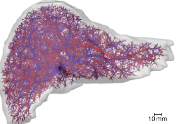
Obtaining Realistic Geometric Models of Organ and Vasculature. A realistic 3D geo-metric model of a human liver and its vascular structures was obtained by applying the same workflow described in [77] for in vivoμCT scans of mouse livers. In summary, an abdominal in vivo MRI scan of a healthy 31-year old male Caucasian was used to segment the liver and its vascular structures [78]. The latter were subsequently skeletonized and converted to a graph representation using a semi-automatic procedure [78]. The vascular graphs were simplified to strictly bifurcative trees with cylindrical edges as described in [79]. They were refined algorith-mically [80] to the desired degree of detail as described in [79]. For this purpose, the same set of 10 000 end points for the supplying and draining vascular systems were used. Each of these points represents groups of about 53physical lobuli, leading to a total of 1.25 million lobuli, a realistic number [1]. In each group, we assume the same metabolic properties for all sinusoids. The underlying organ mask an the resulting vascular system are visualized inFig 3and pro-vided asS1 Dataset.
For a fully lobular resolution, one would have to take into account how the blood supplied by one portal field is distributed to multiple surrounding central veins, an effect we neglect in the approach here. We could, however, easily incorporate it for applications where such a more detailed draining pattern is of importance.
Our applications involving mouse models presented here did not require 3D geometric models as these examples did not include organ-scale heterogeneity. Such geometric models are available as supporting information to [8] and [77] and could easily be included in the sim-ulations if organ-scale heterogeneity needs to be included.
Sinusoid-Scale Model Building Blocks
The sinusoidal scale is the central building block for our multiscale modeling framework. The processes modeled here, in 1D, are relatively simple, but a suitable adaption of parameters, as described in the model integration below, will still be necessary.
Sinusoidal Blood Flow and Pharmacokinetics Model. For the sinusoidal scale, we again start with the general model form as inEq 2distinguishing flowing and stationary concentra-tion. The 1D advection-reaction for one representative sinusoid can then be expressed as
@t cf cs
" #
þ v@xcf
0
" #
¼E cf
cs
" #!
þ
0
mðcsÞ
" #
ð9Þ
whereEandm, as above, denote the exchange of concentrations between the subspaces and the metabolization, respectively, andvis the one-dimensionalflow velocity. Boundary values at the inflow are those provided by the supplying vascular system, outflowing values at the other end of the sinusoid are computed and passed to the draining vascular system. In the current model version, we in particular neglect diffusion outside the cells, in particular in the space of Disse, as well as exchange between neighboring cells due to gap junctions [81].
For the reaction part ofEq 9, multiple compounds may play a role. On the one hand, one compound may change the exchange or metabolization behavior for another compound if the underlying bio-chemical processes involve such an interdependence. On the other hand, meta-bolization itself can produce metabolites (i.e., other compounds) from compounds.
this blood flow. However, for a representation of the average flow behavior, as intended here, we believe this strong simplification to constant flow velocity to be an appropriate description.
Discretization and Implementation. As in [8], we discretize the advection and reaction parts ofEq 9separately. This avoids a rather technical implementation of a numerical scheme capable of treating both processes simultaneously, even though this is possible even for a non-linear reaction term [83]. The simulation moreover does not require a small time step appro-priate for both processes, but needs approappro-priate time steps for the two processes separately and an appropriate synchronization strategy.
We do not resolve the internal spatial structure of hepatocytes and thus assume them to be well-stirred. It is thus a natural choice to use a resolution of one grid point per hepatocyte for the spatial discretization of the representative sinusoids. This is also the spatial resolution at which sinusoid-scale parameter heterogeneity needs to be given.
Advection:While pure 1D advection problems with constant velocity can be solved analyti-cally, this is no longer possible if a reaction term is present as well, so it needs to be addressed numerically. The simplest implementation of time stepping for the advection part ofEq 9
could be obtained by choosing the time step such that the velocity is one grid cell per time step. This, however, would not allow joint time steps if velocities in different representative sinusoids differ, and might be too large a time step for synchronizing with fast reactions, so we need a numerical advection scheme that can deal with arbitrary velocities. An ideal such discretization scheme would conserve mass and neither introduce numerical diffusion nor create spurious oscillations [84]. However, state-of-the-art methods do not simultaneously satisfy all three properties, so a compromise is needed. For our purposes, we particularly focus on mass conser-vation and avoiding spurious oscillations, which might result in overshoots and negative con-centrations, so we need to accept numerical diffusion effects.
We use a 1D Eulerian-Lagrangian Localized Adjoint Method (ELLAM) [60], going back to [85] with more details on mathematical analysis in [86]. This method was preferred over other discretization schemes for advection [87] as it prevents numerical artifacts [88]. To prevent artificial oscillations, mass lumping as suggested in [89,90] was used. While ELLAM could, in principle, treat more than advection simultaneously [83,91,92], also for non-linear reactions [93], we treat flow, exchange/metabolization, and recirculation separately by appropriate meth-ods. The scheme was implemented in custom C++ code based on own earlier work, Section 1
Fig 3. Human Liver Vascular Dataset.The image shows a visualization of a human liver shape including algorithmically refined vascular structures. The supplying vascular system, comprising portal vein and hepatic artery, is shown inred, the draining vascular system (hepatic vein) inblue.
in the supporting information Text S1 of [8] and [94]. In summary, the ELLAM scheme for advection amounts to solving a linear system of equations to update the concentrations for the compounds present in the blood flow in each time step.
ReactionFor the reaction part ofEq 9, we observed no issues due to stiffness of the ODE systems. So we chose a standard Runge-Kutta-Fehlberg 4th/5th order (RKF45) [61] scheme that automatically adapts the time step size. This method is recommended as a‘good general-purpose integrator’in the GNU Scientific Library [95]. The RKF45 performed well in this case, so we do not need to apply more sophisticated methods as recommended in [96,97]. We used a custom C++ implementation of an RKF45 scheme from [8] to avoid data exchange with external libraries as these ODE solution steps are rather time-critical in the simulation.
Model Integration in Representative Sinusoids
Besides a connection of the models on the distinct scales, an adaption of parameters due to the different dimensionality of the models is necessary. This affects the volume fractions, the respective surface areas and thus the effective permeabilities, and the length of regions along the sinusoid. Moreover, we discuss an additional model fitting step needed if our cellular model was not parametrized for the model structure involving representative sinusoids.
One-Dimensional Representation of Sinusoids. To account for increasing sinusoid diameter from portal fields to central veins in a 1D representation of the blood flow in 3D lobuli, we need to find an appropriate representation. As variations of the processes in longitu-dinal direction of the lobulus are of minor importance, we can restrict our view to 2D cross sec-tions of lobuli. Mathematically, the goal of this subsection is to describe how parameters of the PBPK liver submodel need to be adapted. This adaption will involve scaling some of the param-eters and replacing the constant volume fractionsφi,i2{rbc, pls, int, cell}, by volume fractions
ψi(λ) depending on the positionλalong the sinusoid.
For this purpose, our approach is to consider one physiological sinusoid starting from the portal field. As it combines with other sinusoids towards the central vein, the blood flow from the one, portally starting, sinusoid is only a certain fraction between 0 and 1 of the blood flow through the centrally ending sinusoid. For the lack of more detailed data, we assume that the flow velocity does not change along the physiological sinusoids. Moreover, we assume that the physiological sinusoids are surrounded by an interstitial and a cellular layer of constant width, independent of the sinusoid radius.
Radii of periportal and pericentral sinusoids in mice arersin,pp= 4.4μm andrsin,pc= 6.85
μm [98], respectively. This range is similar to sinusoidal diameters of 7 and 15μm reported in [1], so we will use the following formulas for both humans and mice. Assuming a linear increase of the cross section area, the sinusoidal radius can be computed as
A⌀;sinðlÞ ¼A⌀;sin;ppþlðA⌀;sin;pc A⌀;sin;ppÞ ¼pr 2
sin;ppþlðpr 2 sin;pc pr
2
sin;ppÞ ð10aÞ
rsinðlÞ ¼
ffiffiffiffiffiffiffiffiffiffiffiffiffiffiffiffiffi
A⌀;sinðlÞ p
r
¼ ffiffiffiffiffiffiffiffiffiffiffiffiffiffiffiffiffiffiffiffiffiffiffiffiffiffiffiffiffiffiffiffiffiffiffiffiffiffiffiffiffiffiffiffiffir2 sin;ppþlðr
2 sin;pc r
2 sin;ppÞ
q
ð10bÞ
whereλindicates the position along the sinusoid in units of sinusoid length, i.e.,λ= 0 at the periportal end andλ= 1 at the pericentral end.
For the thickness of the interstitium and the representative cellular layer, denoted bywint
sinusoidal cross-section area, i.e., to the radiusrsin, avg=rsin(0.5) = 5.757μm. We then compute
wint¼
ffiffiffiffiffiffiffiffiffiffiffiffiffiffiffi
1þφ
int
φsin
s
1
!
rsin;avg¼3:187μm ð11aÞ
wcell¼
ffiffiffiffiffiffiffiffiffiffiffiffiffiffiffiffiffiffiffiffiffiffiffiffiffiffiffiffi
1þφ
cellþφint
φsin
s ffiffiffiffiffiffiffiffiffiffiffiffiffiffiffiffiffiffiffi
φsinþφint
φsin
s !
rsin;avg¼8:001μm ð11bÞ
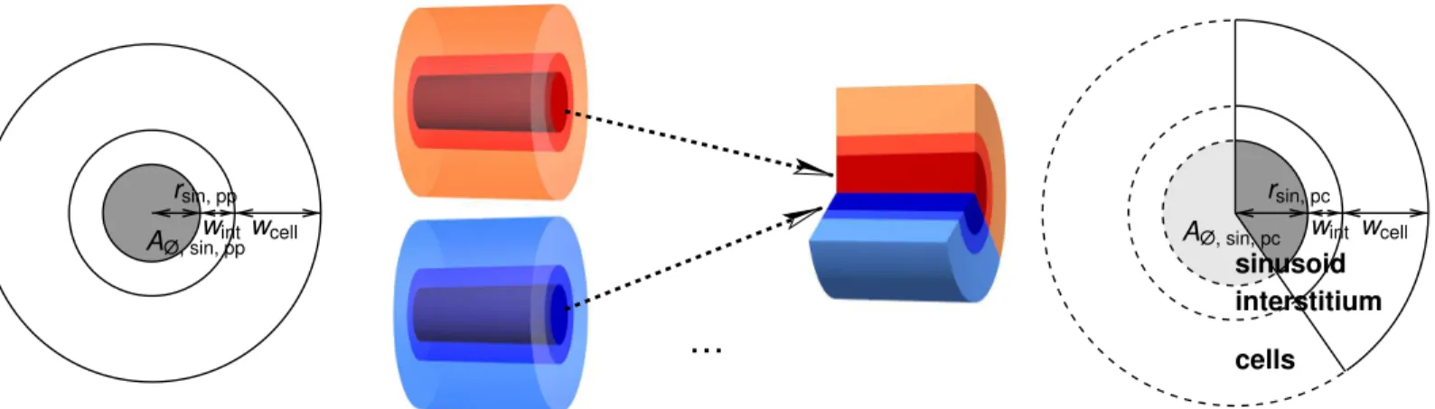
Note that these values refer to volumes representative for the physiological interstitium and cells and are not meant as their precise actual sizes, in particular for the cells. The radii and these thicknesses are illustrated inFig 4.
Using Eqs10and11, the variation of the volume fractions along the representative sinusoid can be expressed as
csinðlÞ ¼ p½rsinðlÞ 2
p½rsinðlÞ þwintþwcell
2 ð12aÞ
crbcðlÞ ¼φrbc
φsin
csinðlÞ ð12bÞ
cplsðlÞ ¼φpls
φsin
csinðlÞ ð12cÞ
cintðlÞ ¼p½rsinðlÞ þwint 2
p½rsinðlÞ 2
p½rsinðlÞ þwintþwcell
2 ð12dÞ
ccellðlÞ ¼p½rsinðlÞ þwintþwcell 2
p½rsinðlÞ þwint 2
p½rsinðlÞ þwintþwcell2 ð12eÞ
The contribution of the periportally starting sinusoid to the representative sinusoid at posi-tionλis given by the ratio of the cross section areas,
rðlÞ ¼p½rsinð0Þ 2
p½rsinðlÞ
2 ¼
r2 sin; pp
½rsinðlÞ
2: ð13Þ
We refer toFig 4for a sketch of this interpretation of the contributions. The inverse of this con-tribution is needed when determining the represented volume by one section of the representa-tive sinusoid. In addition, permeabilities relating to surface areas need to be scaled by a factor derived fromρ(λ), taking into account the circumference of the representative sinusoid at posi-tionλand the fraction of represented there,
sðlÞ ¼ 2prsinðlÞ 2prsinð0:5Þ
rðlÞ
rð0:5Þ: ð14Þ
These adaptions imply a modification of the exchange termEq 3to
EðlÞ ¼
Prbc;pls krbc;plscrbcðlÞ
þPrbc;pls
crbcðlÞ 0 0
þPrbc;pls krbc;plscplsðlÞ
Prbc;pls cplsðlÞ þ
sðlÞPpls;int cplsðlÞ
þsðlÞPpls;int
kpls;intcplsðlÞ 0
0 þsðlÞPpls;int
cintðlÞ
sðlÞPpls;int kpls;intcintðlÞþ
sðlÞPint;cellkint cintðlÞ
þsðlÞPint;cellkcell cintðlÞ
0 0 þsðlÞPint;cellkint
ccellðlÞ
sðlÞPint;cellkcell ccellðlÞ
2 6 6 6 6 6 6 6 6 6 6 6 6 6 6 4 3 7 7 7 7 7 7 7 7 7 7 7 7 7 7 5 ð15Þ
whereas the metabolization termEq 4is unaffected.
One-Dimensional Representation of Sinusoid-Scale Heterogeneity. A zonation of meta-bolic capabilities is typically determined by staining enzymes in histological slices. These images are evaluated by measuring the total cross-section area of different lobuli and the corre-sponding areas of different staining result. For an enzyme near, e.g., the central veins, the anal-ysis thus allows defining a pericentral area ratioApc/A;, whereas we need a pericentral length
ratiolpc/lrep. sin.for the representative sinusoid models. We view lobuli as cylinders around
their respective central vein, which is certainly a simplification from 3D to 2D, but a suitable approximation of the actual polygonal shape of lobuli [99]). Then, we can easily convert from central circular area to central length via
Apc
A;
¼ pl
2 pc pl2
rep: sin:
) lpc lrep: sin:
¼ ffiffiffiffiffiffiffi Apc A; s : ð16Þ
This conversion also applies when considering the zonation of pathological changes as these can be determined similarly, see, e.g.,Fig 1, or, more generally, any sinusoid-scale parameter heterogeneity.
Let us point out that there is no unique‘periportal’or‘pericentral’zone, they can in particu-lar not necessarily be identified with zones 1 or 3 in the notation of [29,100]. The size of such zones depends on the process considered. In the caffeine example considered in the results
Fig 4. Sketch for the 1D Representation of Sinusoids.The volume rendering in themiddleillustrates our assumption of multiple periportally starting sinusoids contributing to a thicker pericentrally terminating sinusoid. The width of the interstitial and cellular layer is assumed to remain constant along the sinusoid. The sinusoidal cross-section sketches on theleftandrightshow that this also has an effect on the respective surface areas, which has an influence on the respective effective permeabilities.
section, there are two pericentral regions: one of fixed size where the enzyme Cyp1a2 is expressed, another one of variable size which is affected by necrosis.
From Well-Stirred to Representative Sinusoid Models. Frequently, the PK parameters are fitted for a well-stirred organ-scale model rather than a spatially resolved representative sinusoid model already taking into account the adaptions described by Eqs15and16. In this case, they cannot be used immediately for the cellular scale in representative sinusoids. Our approach is to rescale parameters dominantly causing the differences such that the liver out-flow concentrations as model output from the organ-scale homogeneous representative sinu-soid model are close to outflow concentrations from the well-stirred organ-scale model. No exact match can be expected here, the sinusoid-scale model is designed to represent the transit time and also exhibits some mixing and other effects due to the advection simulation.
This adaption should clearly be independent of the inflow profile considered. If we were dealing with a linear time-invariant (LTI) system, we could simply determine the impulse responses, i.e., the model output when using a Diracδimpulse as input, of the two models and use these for comparison. The ODE systems considered here, however, are not necessarily lin-ear, so standard methodology for LTI systems (see, e.g., Chapter 2 in [101]) cannot be applied. Instead, we make use of the following pragmatic approach. Assuming that the system behaves approximately linearly for our ranges of input, we consider an inflow profile roughly approxi-mating aδimpulse. We then fit a scaling factor for the dominating coefficients in the ODE sys-tem so that an appropriate deviation is minimized. We will specify this in the results section for our insulin example. This optimization is performed by iterative interval nesting until a given tolerance is reached.
Zonated and Organ-Scale Heterogeneous Pathological States of the
Liver
We now consider two proofs of concept how pathophysiological changes can be taken into account in our model. Steatosis is an example that can occur zonally, organ-scale heteroge-neous form, and the combination thereof. Necrosis after CCl4intoxication occurs in zonal
form in a rather homogeneous form across the liver. The damage happens on a time scale of hours and the liver regenerates within days, so we here consider the time dynamics of this path-ological state.
Simplified Steatosis Model. Steatosis is a common liver disease in humans, it is often caused by alcohol abuse, diabetes, protein malnutrition, obesity or the consequence of other pathological conditions [102]. In steatotic livers, lipids accumulate in the cellular subspace [103]. Most often, this happens pericentrally, but the lipid deposition can also occur in the peri-portal zone, see [104] and the references therein. In addition, an organ-scale heterogeneity between different sinusoids can be observed [105].
Model Perturbation:We represent the effect of steatosis as a change in the equilibrium between cells and interstitium via the respective partition coefficientκcell, healthy=κcellin the PBPK equationEq 3in the same manner as presented in [8]: LetΔsbe the lipid accumulation due to steatosis, thenκcell(Δs) is computed fromκ
cell, healthyvia
kcellðDsÞ ¼ 1
kcell; healthyþ
10logP 1
ccellðlÞ Ds
! 1
ð17Þ
permeabilities [107], any changes in microcirculation [108,109], organ size (as shown in Table 6 in [110]), and any other effects of steatosis on the organ and the whole organism.
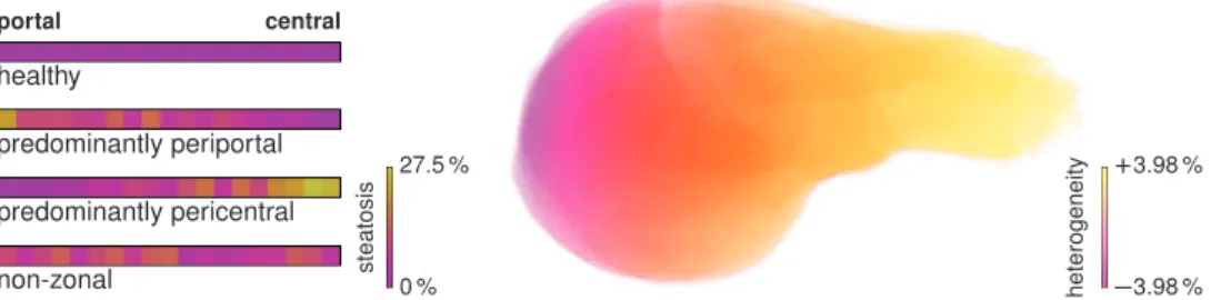
Synthetic Steatosis Data:The steatosis data used here are synthetic datasets based on experimental observations from the literature. Besides the healthy case (no steatosis), we con-sider three types of zonation: predominantly periportal (similar to‘zone 1’in the terminology of Fig 1 in [29]), predominantly pericentral (‘zone 3’), and non-zonal (‘panacinar’or‘azonal’). For this purpose, we assume a total fat accumulation of 9.2% of the liver volume, correspond-ing to stage 2 steatosis as observed in [111]. We assign pseudo-random [112] steatosis values Δsto each zone, uniformly distributed in the interval 0.092(ρ(λ))−1zz(λ)[(1−0.69), (1
+ 0.69)] where 0.69 is the coefficient of variation reported in [111], the factorρ(λ) fromEq 14
in the denominator cancels when computing the total lipid content, andzz(λ) controls the
zonation via
zzðlÞ ¼
1 non zonal case
2 2l predominantly periportal case
2l predominantly pericentral case
ð18Þ
8 > <
> :
Examples for these zonated states of steatosis are visualized inFig 5.
For introducing an organ-scale heterogeneity, we multiply the ranges above by an additional factor
zhðx;y;zÞ ¼1þ0:0398x ðxminþxmaxÞ=2
ðxmin xmaxÞ=2
ð19Þ
wherexminandxmaxare the smallest and largestxcoordinate of the organ. This factor leads to
a gradient in the steatosis profile with a difference of 23.98% between the leftmost and right-most point, given by the smallest and largestxcoordinate, respectively. The value 3.98% is the mean maximum difference between left and right liver as reported in [105] for type-2 diabetic patients, where lower steatosis values are present on the left. A volume rendering inFig 5
shows this macroscopic lateral steatosis gradient.
Simplified Regeneration Model. A frequently used experimental protocol to study toxic liver damage is the administration of CCl4in animals [28]. It induces a necrotic pericentral
zone [34], similar to effects of acetaminophen overdoses [113], a frequent cause for acute liver failure in humans [114].
Model Perturbation:In a similar manner as in [8], we represent the effect of the necrotic area by replacing the cellular volume by interstitial space, changing the volume fractions in the PK equationEq 3. As the actual metabolization only takes place in the cellular volume, this effectively prevents metabolization in the necrotic zone. Let us point out that this is again a strongly simplified model. It explicitly ignores any interaction of the CCl4and its metabolites
with the compound, any effects of the fragments of the dead cells, any differences in the meta-bolic capabilities of the regenerating cells to those of the cells natively at the respective position, and any additional influence of the CCl4administration on the whole organism. For a more
detailed model of the interplay of regeneration and metabolism we refer to [115].
Synthetic Necrosis Data:A CCl4dose of 1.6 mg g
−1body weight leads to necrotic areas
area as input for our simulations is shown inFig 6. A necrosis value between 0% and 100% is proportionally mapped to a change of volume fractions as described above.
Applications and Results
We now show three example applications using our four-scale modeling and simulation frame-work. These applications were chosen to cover a wide range of species, compounds, pathologi-cal conditions, simulation scenarios, and pharmacologipathologi-cally and physiologipathologi-cally relevant output quantities. We first considered the clearance of midazolam in a healthy and a steatotic human liver where both zonation within sinusoids and organ-scale heterogeneity of the steato-sis were present. Next, we addressed the clearance of caffeine in mice where the metabolization was zonated already in healthy livers. During the regeneration after CCl4intoxication, which
induces a zonal necrosis, an additional zonal pathophysiological change of the metabolization was taken into account, leading to different half-lives of the same amount of caffeine in the body. Finally, we show results of a parameter study investigating how sinusoid-scale spatially heterogeneous patterns of different cell entities influenced the uptake of insulin in mouse livers, representing the cell variation along a single sinusoid. Here, we evaluated how physiologically released periodic pulses were damped by the liver.
Fig 5. Steatosis Heterogeneity.Theleftimages show four examples of different synthetic zonated patterns of steatosis in humans, visualized on a color scale from violet to yellow, corresponding to 0% to 27.5% steatotic lipid accumulation. The three steatotic states correspond to the same total lipid accumulation of 9.2%. The volume rendering on therightvisualizes the organ-scale gradientζhwith a difference of 7.96% lateral direction for a human liver.
doi:10.1371/journal.pone.0133653.g005
Fig 6. Necrosis and Regeneration.The plot shows how the spatial extent of the necrotic region evolves according to our model of the effect of CCl4intoxication along a representative sinusoid of a mouse liver. The
representative hepatocytes are separated by vertical black lines in this plot, A color range from white to red indicates zero to full necrotic damage of the respective representative hepatocyte. Necrosis develops during the first day, until a maximally necrotic state is attained. Subsequent regeneration starting on the second day leads to a shrinkage of the necrotic region until the end of day 7.
The midazolam and caffeine models are of the structure presented inEq 3. The parameters needed therein and inEq 4for the two compounds are listed inTable 2. The insulin model, in contrast, has a different structure presented below inEq 21. It was moreover parametrized using experimental ex vivo data for cells in a non-flowing medium, requiring a model and parameter conversion as described above for being able to use the model in our representative sinusoid approach. The steatotic perturbation in the midazolam model involved an organ-scale heterogeneity and was thus investigated using a realistic geometric model of a human liver and its vascular structures. The other two examples considered inhomogeneity only at the lobular scale and thus did not require organ-scale geometric models.
Midazolam Metabolism of Human Steatotic Livers
Midazolam is a sedative and anesthetic induction agent [116]. It is metabolized by the enzyme CYP3A4 [117] only expressed in the pericentral region [118].
Pharmacokinetics Model. Based on Fig 1 in [119], we estimated the size of the pericentral region of CYP3A4 expression to be be slightly over 50% of the lobular cross-section area. ByEq 16, this pericentral area corresponds to 14 of 19 hepatocytes performing the metabolization.
We used the available software [59] to establish a human PBPK model for midazolam based on physiochemical parameters from [120] and the Human Metabolome Database [121] as well as to determine the partition coefficientsκand the permeabilitiesPlisted inTable 2. The parametersVcell
max,K
cell
m , and logPwerefitted to data manually derived from Fig 2 in [122].
This model was parametrized for a 19-zonal liver model matching our representative sinu-soid model for humans, the parameters could thus be used without further adaption.
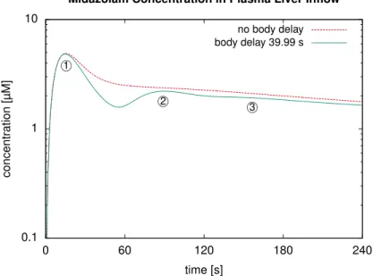
Simulation Results: Influence of the Body Delay. First, we represented the healthy liver by a single representative sinusoid and used an intravenous bolus injection of 11.42 mg as in the experiments underlying the data used above for fitting. Here, we determined the simulated midazolam concentrations in the plasma entering the liver via the portal vein, comparing a recirculation model as described above to one without delay during the recirculation.
Results for this simulation inFig 7show that, without recirculation delay, our model failed to predict reoccurring peaks of the second and third pass. With nonzero recirculation delay, these peaks were captured with a physiologically reasonable temporal delay. In our case, we observed a temporal spacing of about 75 seconds between the first two peaks. This is clearly longer than a time span of approximately 23 s which can be estimated from Fig 4 in [63]. The literature data is for a different compound with potentially different PK characteristics
Table 2. Pharmacokinetics Parameters.For the two compounds whose pharmacokinetics is described by Eqs3and4, the table lists the respective PK parameters: partition coefficientsκ, permeabilitiesP, metaboli-zation parametersVcell
maxandK cell
m ; the lipophilicity logP
Compound Species Midazolam Human Caffeine Mouse
κrbc,pls[–] 3.90310−1 5.85010−1
κpls,int[–] 3.84210−1 8.73510−1
κint[–] 6.24610−2 9.73110−1
κcell[–] 1.06010−2 1.192100
Prbc,pls[s−1] 9.87110−3 4.01710−3
Ppls,int[s−1] 6.460100 1.548102
Pint,cell[s−1] 6.776100 1.039100
Vcell max[mM s
−1] 2.53110−7 6.60910−3
Kcell
m [mM] 1.010
−8 4.5210−1
logP[–] 3.107100 −7.010−2
throughout the body, which could account for part of the difference. Mainly, the difference is due to our recirculation model not yet accurately representing the flow delays by different organs and for different paths through the body. However, a more accurate recirculation delay is beyond the scope of this article where we focus on a detailed liver model and consider the simplified recirculation delay sufficient for our purposes. In particular, we did not simply pick our recirculation delayτrec totalfromEq 1such that the time span between two peaks matches
the literature values. Such an approach would merely hide the inaccuracy described and would probably lead to incorrect amplitude of the second peak because flow delays by slower paths through the body would not be represented correctly and the circulation speed of the entire mass would be overestimated.
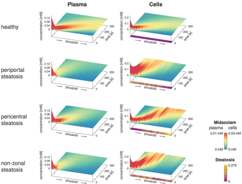
Results for the Zonated, Organ-Scale Homogeneous Model. We next assumed infusion of the same dose of midazolam into the blood plasma flowing through the portal vein within 5 seconds. In this case, we determined the simulated spatio-temporally resolved concentration profiles along the sinusoid in the healthy, predominantly periportal, predominantly pericentral, and non-zonal steatotic cases.
InFig 8, we can clearly observe the influence of the different steatosis patterns on the spa-tio-temporal midazolam distribution. As expected fromEq 17, a higher accumulation of mida-zolam was predicted for the steatotic regions. In the plots, the apparent velocity of the peak is particularly noteworthy with an apparent transit time of about 200 seconds for the healthy state, and slower apparent velocity for the steatotic states. We emphasize that this time scale is different from the blood flow velocity, for which the transit time is 13.6 s as given inEq 6, i.e., significantly shorter and according to our assumptions in particular independent of the steatosis.
The simulation results here clearly depend on how the randomized steatosis patterns were chosen, i.e., on the seed value of the pseudo-random number generator. While it would be rea-sonable to investigate how sensitive the results are to the seed, and more generally to all the
Fig 7. Influence of the Body Delay.For an intravenous bolus injection in our human whole-body model with a liver described by a single representative sinusoid, the plot shows the simulated midazolam concentration in the blood plasma at the liver inflow. Setting the temporal delay of the recirculation to zero (dashed line) shows that the delay in the model is indispensable for a correct prediction of recurring peaks for a second and third pass, indicated by circled numbers in the plot.
model parameters, such a sensitivity analysis is beyond the scope of the present exemplary use case.
Results for the Zonated, Organ-Scale Heterogeneous Model. Moreover, we considered a liver model using 10 000 representative sinusoids with the vasculature as shown inFig 3. In this case, each representative sinusoid had its individual steatosis pattern (predominantly peri-portal predominantly pericentral, non-zonal), additionally the lateral organ-scale gradient as given inEq 19was present. Due to the large number of sinusoids, the influence of the individ-ual patterns, as discussed above, averaged out. For these simulations, we again assumed an infusion into the blood plasma flowing through the portal vein within 5 seconds. We then
Fig 8. Spatio-Temporal Midazolam Concentration Profiles.The surface plots show the spatio-temporal evolution of the midazolam concentrations in the blood plasma and the hepatocytes along representative sinusoids assuming an infusion of duration 5 seconds into the portal vein, comparing the healthy reference case with three different steatotic cases with the same total amount of lipid accumulation. While the height in the graph covers the total
concentration ranges, the color highlights differences in a lower range of concentrations, emphasizing the differences between the four cases. In addition, the steatosis patterns along the sinusoids are shown below the cellular concentrations. Differences in the transit time of the peak are due to different extent of storage and release of the midazolam due to the steatotic lipid accumulations. This should not be mistaken for the blood flow transit time, which is 13.6 s for all four cases and thus much shorter than the peak transit time.