Idealized computational models for auditory receptive fields.

Idealized Computational Models for Auditory

Receptive Fields

Tony Lindeberg1*, Anders Friberg2

1Department of Computational Biology, School of Computer Science and Communication, KTH Royal Institute of Technology, Stockholm, Sweden,2Department of Speech, Music and Hearing, School of Computer Science and Communication, KTH Royal Institute of Technology, Stockholm, Sweden

*tony@csc.kth.se

Abstract

We present a theory by which idealized models of auditory receptive fields can be derived in a principled axiomatic manner, from a set of structural properties to (i) enable invariance of receptive field responses under natural sound transformations and (ii) ensure internal con-sistency between spectro-temporal receptive fields at different temporal and spectral scales. For defining a time-frequency transformation of a purely temporal sound signal, it is shown that the framework allows for a new way of deriving the Gabor and Gammatone fil-ters as well as a novel family of generalized Gammatone filfil-ters, with additional degrees of freedom to obtain different trade-offs between the spectral selectivity and the temporal delay of time-causal temporal window functions. When applied to the definition of a second-layer of receptive fields from a spectrogram, it is shown that the framework leads to two ca-nonical families of spectro-temporal receptive fields, in terms of spectro-temporal deriva-tives of either spectro-temporal Gaussian kernels for non-causal time or a cascade of time-causal first-order integrators over the temporal domain and a Gaussian filter over the log-spectral domain. For each filter family, the spectro-temporal receptive fields can be either separable over the time-frequency domain or be adapted to local glissando transformations that represent variations in logarithmic frequencies over time. Within each domain of either non-causal or time-causal time, these receptive field families are derived by uniqueness from the assumptions. It is demonstrated how the presented framework allows for computa-tion of basic auditory features for audio processing and that it leads to prediccomputa-tions about au-ditory receptive fields with good qualitative similarity to biological receptive fields measured in the inferior colliculus (ICC) and primary auditory cortex (A1) of mammals.

Introduction

The information in sound is based on variations in the air pressure over time, which for many sound sources can be modelled as a superposition of sine wave oscillations of different frequen-cies. To capture this information by auditory perception or signal processing, the sound signal has to be processed over some non-infinitesimal amount of time and in the case of a spectral OPEN ACCESS

Citation:Lindeberg T, Friberg A (2015) Idealized Computational Models for Auditory Receptive Fields. PLoS ONE 10(3): e0119032. doi:10.1371/journal. pone.0119032

Academic Editor:Sonja Kotz, Max Planck Institute for Human Cognitive and Brain Sciences, GERMANY

Received:April 4, 2014

Accepted:January 24, 2015

Published:March 30, 2015

Copyright:© 2015 Lindeberg, Friberg. This is an open access article distributed under the terms of the Creative Commons Attribution License, which permits unrestricted use, distribution, and reproduction in any medium, provided the original author and source are credited.

Data Availability Statement:The main contributions of this paper are theoretical and all relevant data for the paper are contained within the paper.

analysis also over some range of frequencies. Such a region over time or over the spectro-tem-poral domain is referred to as a temspectro-tem-poral or spectro-temspectro-tem-poralreceptive field(Aertsen and Johannesma [1]; Theunissen et al. [2]; Miller et al. [3]; Fritz et al. [4]).

If one considers the theoretical or algorithmic problem of designing an auditory system that is going to analyse the variations in air pressure over time, one may ask what types of auditory operations should be performed on the sound signal. Would any operation be reasonable? Spe-cifically, regarding the notion of receptive fields, what types of temporal or spectro-temporal receptive field profiles would be reasonable? Is it possible to derive a theoretical model of how receptive fields“ought to”respond to auditory signals?

In vision, the corresponding problem of formulating a theoretical model for visual receptive fields (Lindeberg [5]) can be addressed based on a framework developed in the area of comput-er vision known asscale-space theory(Iijima [6]; Witkin [7]; Koenderink [8]; Koenderink and van Doorn [9,10]; Lindeberg [11–14]; Sporring et al. [15]; Florack [16]; ter Haar Romeny [17]). A paradigm that has been developed in this field is to imposestructural constraintson the first stages of processing that reflectsymmetry propertiesof the environment. Interestingly, it turns out to be possible to substantially reduce the class of permissible image operations from such arguments, and it has been shown that biological receptive fields as measured in the lateral geniculate nucleus (LGN) and the primary visual cortex (V1) of higher mammals (Hubel and Wiesel [18–20]; DeAngelis et al. [21,22]; Conway and Livingstone [23]; Johnson et al. [24]) can be well modelled by idealized scale-space operations (Young et al. [25,26]; Lin-deberg [5,27]).

The subject of this article is to show how a corresponding normative theory for receptive fields can be developed for auditory stimuli, and how idealized models of auditory receptive fields can be derived in a principled manner by applying scale-space theory to auditory signals. Our aim is to express auditory operations that are well localized over time and frequencies and which allow for well-founded handling of temporal phenomena that occur at different tempo-ral scales as well as receptive fields that operate over different ranges of frequencies in such a way that operations over different ranges of frequencies can be related in a

well-defined manner.

When applied to the definition of spectrograms, alternatively to the formulation of an ideal-ized cochlea model, the scale-space approach can be used for deriving the Gabor (Gabor [28]; Wolfe et al. [29]; Lobo and Loizou [30]; Qiu et al. [31]; Wu et al. [32]) and Gamma-tone (Johannesma [33]; Patterson et al. [34]; Hewitt and Meddis [35,36]) approaches for computing local windowed Fourier transforms as specific cases of a complex-valued scale-space transform over different frequencies. In addition, the scale-space approach to defining spectrograms leads to a new family ofgeneralized Gamma-tone filters, where the time constants of the individual first-order integrators coupled in cascade are not equal as for regular Gamma-tone filters but instead distributed logarithmically over temporal scales and allowing for different trade-offs in terms ofe.g. the frequency selectivity of the spectrogram and the temporal delay of time-causal receptive fields.

When applied to a logarithmic transformation of the spectrogram, as motivated from the desire of handling sound signals of different strength (sound pressure) in an invariant manner and with a logarithmic transformation of the frequencies as motivated by the desire of enabling invariance properties under a frequency shift, such as transposing a musical piece by one oc-tave, we will show how this theory also allows for the formulation of spectro-temporal receptive fields at higher levels in the auditory hierarchy in terms of spectro-temporal derivatives of spec-tro-temporal smoothing operations as obtained from scale-space theory.

It will be demonstrated how such second-layer receptive fields can be used forcomputing basic auditory featuressuch as onset detection, partial tone enhancement and formants, and collection and analysis, decision to publish, or

preparation of the manuscript.

specifically how different types of features can be obtained at different temporal scalesτ, spec-tral scalessand how this theory naturally also leads to a glissando parametervthat represents how logarithmic frequenciesνmay vary over timetaccording to a local linear approximation ν0_=ν+vt.

Compared to the more common approach of computing auditory features in digital signal processing by local windowed fast Fourier transforms (FFT), we argue that the proposed theory provides a way to avoid artifacts of performing the computation in temporal blocks that later have to be combined again. Furthermore, by the built-in covariance properties of the model under temporal shifts, variations in sound pressure, frequency shifts and glissando transforma-tions, the proposed approach allows forprovable invariance propertiesunder such transforma-tions of sound signals.

It will also be shown how idealized models of spectro-temporal receptive fields as obtained from the presented theory in terms of spectro-temporal derivatives of spectro-temporal scale-space kernels can be used for generatingpredictions of auditory receptive fields that are qualita-tively similar to biological receptive fieldsas measured by cell recordings in the inferior collicu-lus (ICC) and the primary auditory cortex (A1) (Miller et al. [3]; Qiu et al. [31]; Machens et al. [37]; Andoni et al. [38]; Elhilali et al. [39]; Atencio and Schreiner [40]).

Outline of the presentation

The presentation is organized as follows: The section“Structural requirements on temporal re-ceptive fields”describes basic constraints on temporal receptive fields as motivated by the de-sire of capturing temporal structures at different temporal scales in a theoretically well-defined manner. The section“Scale-space concepts for purely temporal domains”then describes the temporal scale-space concepts that satisfy these properties, with a distinction on whether the auditory processing operations are required to be time-causal or not. For off-line processing of pre-recorded sound signals, we may take the liberty of accessing the virtual future in relation to any pre-recorded time moment, whereas one in a real-time situation has to take the fact that the future cannot be accessed into explicit account. Thereby, we obtain different theories de-pending on whether time is treated in a non-causal or a time-causal manner.

In the section“Multi-scale spectrograms for auditory signals”we apply these temporal scale-space theories to the definition of multi-scale spectrograms by the formulation of locally windowed Fourier transforms of different temporal extent to be able to capture temporal phe-nomena at different temporal scales. The section“Receptive fields defined over the spectro-gram”develops a corresponding theory for spectro-temporal receptive fields applied to the spectrogram, and it is shown how auditory receptive fields over the spectro-temporal domain can be expressed in an analogous way to how visual receptive fields are defined over space-time, with the conceptual difference that the two spatial dimensions in vision are replaced by a logarithmic frequency dimension. Specifically, we demonstrate how basic auditory features can be computed in this way from spectro-temporal derivatives of idealized receptive fields as ob-tained from the auditory scale-space theory.

The section“Relations to biological receptive fields”gives examples of how biological audi-tory receptive fields can be modelled by the proposed theory. The section“Relations to previ-ous work in audio processing”relates the presented theory to previous approaches in audio processing, and the section“Summary and discussion”concludes with an overall summary of the contributions in the paper, implications of the theory and directions for future work.

analysis of the temporal delays of the time-causal receptive fields. Finally, the section “Compu-tational implementation”shows how the presented continuous theory can be transferred to a discrete implementation while still preserving the theoretical scale-space properties, and there-by allowing for theoretically well-founded digital implementatione.g. for digital audio signal processing or computational modelling of auditory perception.

Structural requirements on temporal receptive fields

In the following, we will describe a set of structural requirements concerning temporal recep-tive fields for a general sensory system that processes a scalar time-dependent signal regarding (i) the measurement of sensory data with its close relationship to the notion of temporal scale, (ii) internal derived representations of the signal that are to be computed by a general sensory system, and (iii) the special nature of time in terms of temporal causality and

temporal recursivity.

If we regard the sensory signalfas defined on a one-dimensional continuous temporal axisf :R_!R_{, then the problem of defining a set of early sensory operations can be formulated as}

finding a family of operatorsT_τthat are to act onfto produce a family of new intermediate rep-resentations of the signal

Lð; tÞ ¼T_t fðÞ ð1Þ

which are also to be defined as functions onR_{,i.e.,L(;τ) :}R_!R_.

(InEquation (1), the symbol“”at the position of the first argument ofLis a place holder to emphasize that in this relation,Lis regarded as a function and not evaluated with respect to its first argumentt. The following semi-colon emphasizes the different natures of the temporal co-ordinatetand the filter parameterτ.)

The evaluation of one (specific example) functionLcan be interpreted as the response of a (set of) sensory neurons in biology or as an internal representation in a temporal signal pro-cessing system that processes temporal information. Combined with additional propro-cessing over frequencies, we will later use such internal representations for modelling neurons in the inferior colliculus (ICC) and the primary auditory cortex (A1).

General scale-space axioms for temporal receptive fields

Linearity. If we want the initial auditory processing stages to make as few irreversible deci-sions as possible, it is natural to requireT_τto belinearsuch that

T_{tða1f1þa2f2Þ ¼a1}T_tf1þa2T_{tf2 ð2Þ}

holds for all functionsf1,f2:R!Rand all scalar constantsa1,a22R. The motivation for

avoiding early irreversible decisions is that we would as much as possible like to preserve an isomorphic mapping to the input, not losing important information.

Linearity also implies that a number of special properties of receptive fields (to be developed below) transfer to temporal derivatives of these and do therefore imply that different types of time-dependent structures in the signal will be treated in a similar manner irrespective of what types of linear filters they are captured by.

reparameterization of the sensor signalIaccording to a self-similar power law for someα>0

fðtÞ ¼ðIðtÞÞa ð3Þ

or a self-similar logarithmic transformation

fðtÞ ¼ log IðtÞ I0

ð4Þ

defined relative to some reference levelI0. Both of these transformations are self-similar in the

sense that (i) they are well-behaved under rescalings of the measurement domainI(t)7!a I(t) fora>0 and (ii) the local magnification/compression around any measurement value as de-fined from the derivative also follows a self-similar power law.

Temporal shift invariance. Let us requireT_τto be ashift-invariant operatorin the sense that it commutes with the temporal shift operatorS_Δtdefined by (S_Δtf)(t) =f(t−Δt), such that

T_tðS_Dt fÞ ¼S_DtðT_tfÞ ð5Þ

holds for allΔt2R_{. The motivation behind this assumption is the basic requirement that the}

representation of a sensory event should be similar irrespective of when it occurs.

Convolution structure. Together, the assumptions of linearity and shift-invariance imply

that the internal representationsL(;τ) are given byconvolution transformations(Hirschmann and Widder [41])

Lðt; t_{Þ ¼ ð}Tð; t_Þ fÞðtÞ ¼

Z

x2R

Tðx; t_Þfðt x_Þdx _ð6Þ

whereT(;τ) denotes some family of convolution kernels. These kernels and their temporal de-rivatives can also be referred to as temporal receptivefields.

Regularity. To be able to use tools from functional analysis, we will initially assume that both the original signalfand the family of convolution kernelsT(;τ) are in the Banach space L2(R_{),i.e. thatf2L}2₍R_{) andT(;τ)2L}2₍R_{) with the norm}

kf k2 2¼

Z

t2R jfðtÞj2

dt: ð7Þ

Then, also the intermediate representationsL(;τ) will be in the same Banach space, and the operatorsT_{τcan be regarded as well-defined.}

Positivity (non-negativity). Concerning the convolution kernelsT, one may require these

to be non-negative to constitute smoothing transformations

Tðt; tÞ 0: ð8Þ

Normalization. Furthermore, it is natural to require the convolution kernels to be

nor-malized to unit mass

kTð; tÞ k1¼ Z

t2R

Tðt; tÞdt¼1 _ð9Þ

to leave a constant signal unaffected by the temporal smoothing transformation.

Quantitative measurement of the temporal extent and the temporal offset of

offsetm¼_{tby the temporal mean operator}

m¼_t¼MðTð; t_{ÞÞ ¼}

R

t2Rt Tðt; tÞdt

R

t2RTðt; tÞdt

ð10Þ

and the temporal extent by the temporal variance

S¼VðTð; t_{ÞÞ ¼}

R

t2Rðt tÞ 2

Tðt; t_Þdt R

t2RTðt; tÞdt

: ð11Þ

Using the additive properties of mean values and variances under convolution, which hold for non-negative distributions, it follows that

m ¼ MðTð; t1Þ Tð; t2ÞÞ ¼MðTð; t1ÞÞ þMðTð; t2ÞÞ ¼m1þm2; ð12Þ

S ¼ VðTð; t1Þ Tð; t2ÞÞ ¼VðTð; t1ÞÞ þVðTð; t2ÞÞ ¼S1þS2: ð13Þ

Identity operation with continuity. To guarantee that the limit case of the internal scale-space representations when the scale parameterτtends to zero should correspond to the origi-nal sound sigorigi-nalf, we will assume that

lim

t#0 Lð; tÞ ¼limt#0

T_{tf ¼f}: ð14Þ

Hence, the intermediate signal representationsL(;τ) can be regarded as a family of derived representations parameterized by a temporal scale parameterτ.

Semi-group alternatively Markov structure over scale. For such sensory measurements

to be properly relatedbetweendifferent temporal scales, it is natural to require the operatorsT_τ

with their associated convolution kernelsT(;τ) to form asemi-groupoverτ

T_t

1Tt2¼Tt1þt2 ð15Þ

which means that the composition of two kernels from the semi-group should also be a mem-ber of the same family of kernels and with added parameter values

Tð; t_1Þ Tð; t_{2Þ ¼}Tð; t_1þt_2Þ: ð16Þ

Then, the transformation between any different and ordered scale levelsτ1andτ2withτ2τ1

will obey thecascade property

Lð; t_{2Þ ¼} Tð; t₂ t_1Þ Tð; t_1Þ f ¼Tð; t₂ t_1Þ Lð; t_{1Þ ð}17Þ

implying that we can compute the representationL(;τ2) at a coarser scale from the

representa-tionL(;τ1) at anyfiner scale using a similar type of transformation as when computing the

re-presentation at any scale from the original dataf.

For a temporal scale-space representation based on a discrete set of temporal scale levelsτk

(k= 0. . .K), we can alternatively require aMarkov propertyof the form

Tð; t_{kþ1Þ ¼ ð}DTÞð; kÞ Tð; t_{kÞ ð}18Þ

where (ΔT)(;k) represents the transformation between adjacent scale levelsτkandτki+1. Then,

the mapping between any pair of temporal scale levelsm<n

will be given by convolution with the kernel

ðDTÞð; m7!nÞ ¼ n 1

k¼mðDTÞð; kÞ: ð20Þ

The difference between the semi-group and the Markov assumptions is that the semi-group structure forces the transformations between adjacent scales to be independent of the current scale level, whereas the transformations between adjacent scales may vary with scale under the Markov assumption. The reason for relaxing the semi-group structure to a Markov structure is to make it possible to take larger temporal scale stepsΔτkat coarser temporal scales, which will

have important implications for time-causal receptivefields.

A representation of a signal possessing these properties is called atemporal multi-scale representation.

Self-similarity over scale. Regarding the family of convolution kernels used for computing

a multi-scale representation, one may require them to beself-similar over temporal scales, such that all the kernels correspond to rescaled copies

Tðt; tÞ ¼ 1

φðt_ÞT

t φðt_Þ

ð21Þ

of some prototype kernelTfor some transformation ofφ(τ) of the temporal scale parameterτ. The reason for introducing a functionφfor transforming the scale parametersinto a scaling factorφ(τ) over time, is that the semi-group requirement (15) does not imply any restriction on how the parameterτshould be related to sound measurements in dimensions of time—the semi-group structure only implies an abstract ordering relation between coarser and finer scalesτ2>τ1that could also be satisfied for any monotonously increasing transformation of

the scale parameterτ. For the Gaussian temporal scale-space concept (25)–(26) this transfor-mation is given bys_¼φðt_{Þ ¼} ffiffiffiffi

t p

.

Temporal covariance. If the same sensory stimulus is recorded by two sensors that sample

the variations in the stimulus with different temporal sampling rates, or if similar temporal events occur at a somewhat different speed, it seems natural that the auditory system should be able to relate the temporal scale-space representations that are computed from the data.

Therefore, one may require that if the temporal dimension is rescaled by a uniform scaling factorf0_{=Sfcorresponding tof}0_(t0_{) =f(t) witht}0_{=S t, then there should exist some}

transforma-tion of the temporal scaleτ0_{=B(τ) such that the corresponding temporal scale-space}

represen-tations are equal:L0_(t0_;τ0_{) =L(t;τ) corresponding toT}

B(τ)ℬf=ℬTτf. In the case of a discrete set

of temporal scale levels, we cannot however require self-similarity or temporal covariance to hold exactly. At best, we can aim at approximate transformation propertiese.g. in terms of the temporal variance of the temporal scale-space kernels.

Non-creation of new structures with increasing scale. A necessary requirement on a

scale-space representation is that convolution with the scale-space kernelT(;τ) should corre-spond to asmoothing transformationin the sense that coarser scale representations should be guaranteed to constitutesimplificationsof corresponding finer scale representations, so that new structures are not created from finer to coarser scales:

Non-creation of local extrema (zero-crossings). One way of formalizing such a

require-ment for a one-dimensional signalf:R_!R_{, is by the requirement that the number of local}

Specific scale-space axioms for a non-causal temporal domain

Depending on the conditions under which the sensory data is processed, we can consider two types of cases. For pre-recorded signals, we may in principle assume access to the data at all temporal moments simultaneously and thereby apply operations to the signal that would cor-respond to access to virtual future. For real-time signal processing or when modelling biologi-cal perception, there is, however, no way of having access to the future, which imposes fundamental additional structural requirements on a temporal front-end. For pre-recorded temporal signals, we require the following:

Non-enhancement of local extrema. In the case of a continuous scale parameter, one way

of formalizing the requirement of non-creation of new structures in the signal with increasing scale is thatlocal extrema must not be enhanced with increasing scale. In other words, if a point (t0;τ0) is a local (spatial) maximum of the mappingt7!L(t;τ0) then the value must not

in-crease with scale. Similarly, if a point (t;τ0) is a local (spatial) minimum of the mappingt7!L

(t;τ0), then the value must not decrease with scale (seefig. 1). Given the above mentioned

differentiability property with respect to scale, we say that the multi-scale representation con-stitutes ascale-space representationif for a scalar scale parameter it satisfies the following con-ditions (Lindeberg [14,43]):

@tLðt0; t0Þ 0 at any non degenerate local maximum; ð22Þ

@tLðt0; tt0Þ 0 at any non degenerate local minimum: ð23Þ By considering the response to a constant signal, it follows from the requirement of non-en-hancement of local extrema that a scale-space kernel should be normalized to unitL1-norm,

corresponding to the normalization requirement inEquation (9).

Specific scale-space axioms for a time-causal temporal domain

When processing sensory data in a real-time scenario, the following additional temporal re-quirements are instead needed:

Fig 1. Illustration of the notion of non-enhancement of local extrema for a 1-D signal.The requirement of non-enhancement of local extrema is a way of restricting the class of possible filtering operations by formalizing the notion that new structures in the signal must not be created with increasing scale, by requiring that the value at a local maximum must not increase with scale and that the value at a local minimum must not decrease. (Figure from Lindeberg [27].)

Temporal causality. For a sensory system that interacts with the environment in a real-time setting, a fundamental constraint on the convolution kernels (the temporal receptive fields) is that there is no way of having access to future information, implying that the temporal smoothing kernels must betime-causalsuch that the convolution kernel must be zero for any relative time moment that would imply access to the future:

Tðt; tÞ ¼0 if t<0: ð24Þ

The possibly pragmatic solution of using a truncated symmetricfilter offinite support in com-bination with a temporal delay may not be appropriate for a time-critical real-time system, since it would lead to unnecessarily long time delays in particular at coarser temporal scales. Therefore, a dedicated theory for truly time-causal spatio-temporal scale-space concepts is needed.

Time-recursivity. Another fundamental constraint on a real-time system is that it cannot

be expected to keep a full record of everything that has happened in the past. To keep down memory requirements, it is desirable that the computations can be based on a limited internal temporal buffer M(t), which should provide:

• a sufficient record of past information and

• sufficient information to update its internal state in a recursive manner over time as new information arrives.

A particularly useful solution in this context is to use the internal temporal representationsLat different temporal scales as a sufficient temporal memory buffer of the past.

Non-creation of structure in the context of discrete temporal scale levels. For a

tempo-ral scale-space representation involving a discrete set of scale levels only, we build on the re-quirement of non-creation of local extrema as expressed for a one-dimensional temporal signal depending on timetonly. Let us therefore regard a one-dimensional temporal smoothing ker-nelTtimeas atemporal scale-space kernelif and only if the kernel is (i) time-causal and in

addi-tion (ii) for any purely temporal signalf, the number of local extrema inTtimefis guaranteed

to not exceed the number of local extrema inf(Lindeberg and Fagerström [44]).

Scale-space concepts for purely temporal domains

In this section we will describe how the structural requirements listed in the section“Structural requirements on temporal receptive fields”restrict the class of temporal scale-space kernels and thus the class of possible temporal receptive fields.

Non-causal Gaussian temporal scale-space

If, for the purpose of analyzing pre-recorded auditory data, we allow for unlimited freedom of accessing the sensory data at all temporal moments simultaneously, we can apply a similar way of reasoning as has been used for deriving scale-space concepts for image data over a spatial do-main (Iijima [6]; Witkin [7]; Koenderink [8]; Lindeberg [11–14,43]; Sporring et al. [15]; Flor-ack [16]; Weickert et al. [45]; ter Haar Romeny [17]):

Given time-dependent sensory dataf:R_!R_{defined over a one-dimensional temporal}

do-main, let us assume that the first stage of sensory processing as represented by the operatorT_τ

non-enhancement of local extremato hold foranysmooth functionf2C1(R_)\L1₍R_{) and for any}

positive scale directions.

Then, it follows from (Lindeberg [14], theorem 5) that these conditions together imply that the scale-space familyLmust satisfy a diffusion equation of the form

@tL¼

1

2S0@ttL d0@tL ð25Þ

with initial conditionL(t; 0) =f(t) for some positive constantS0and some constantδ0.

Equiva-lently, this spatio-temporal scale-space representation at scaleτcan be obtained by convolution withtemporal Gaussian kernelsof the form

gðt; tÞ ¼ ffiffiffiffiffiffiffiffiffiffiffi1 2pSt

p e

ðt dtÞ2=2t

ð26Þ

withSτ=τS0andδτ=τδ0. Since the parameterS0only corresponds to an unessential

rescal-ing of the temporal scale parameterτ, we will setS0= 1.

To verify that the solutions of the diffusion equation obey non-enhancement of local extrema is straightforward. For a one-dimensional signal the first-order derivative is zero, whereas the value of the second derivative will be positive at local minima and negative at local maxima. Hence, for Gaussian smoothing as governed by the diffusionEquation (25), the derivative with respect to scale is guaranteed to be positive at local minima and negative at local maxima (sufficiency). A less immediate result is that non-enhancement of local extrema also implies that the evolution over scale must be governed by the diffusion equation (necessity) and is proved in (Lindeberg [14]). Graphs of these Gaussian kernels are shown infig. 2. Notably, these kernels are not strictly time causal. To arbitrary degree of accuracy, however, they can be approximated by truncated time-causal kernels, provided that the time delayδis chosen sufficiently long in relation to the temporal scaleτ. Hence, the choice ofδleads to a trade-off between the computational accura-cy of the implementation and the temporal response properties as delimited by a non-zero time delay. This problem, however, arises only for real-time analysis. For off-line computa-tions, the time delay may be set to zero, corresponding to kernels that are mirror symmetricT (−t;s) =T(t;s) through the origin. Thus, the truncated and time-shifted Gaussian kernels can

serve as a simplest possible model for a temporal scale-space representation, provided that the requirements of temporal causality and temporal recursivity can be relaxed.

Derived receptive fields in terms of temporal derivatives. In addition to the zero-order

smoothing kernelT, we have infig. 2also shown its first- and second-order temporal deriva-tivesTtandTtt. Such derivatives of scale-space kernels do also obey desirable structural

Fig 2.The time-shifted Gaussian kernelgðt;t;dÞ ¼1= ffiffiffiffiffiffiffiffiffiffi

2pt

p

expð ðt dÞ2

=2tÞforτ= 1 andδ= 4 with its first- and second-order temporal

derivatives.

properties in terms of linearity, shift invariance and nice properties over scale in terms of non-enhancement of local extrema, with the semi-group property replaced by a cascade property over scale

ð@_taLÞð; t₂Þ ¼Tð; t₂ t₁Þ ð@_taLÞð; t₁Þ ð27Þ

and with the limit case when the temporal scale goes to zero (14) replaced by

lim

t#0 ð@t

aLÞð; tÞ ¼lim t#0 @t

aðT_tfÞ ¼@_taf ð28Þ

provided that the corresponding derivative offexists. Regarding temporal receptivefields that are expressed in terms of derivatives of scale-space kernels, the normalization condition (9) is replaced by the integral of the receptivefield being zero

k ð@_taTÞð; tÞk₁¼

Z

t2R

ð@_taTÞðt; tÞdt¼0: ð29Þ

In all other major respects, such receptivefields satisfy essential scale-space properties in terms of non-creation of new structures with increasing scale in the sense that local extrema in the receptive field response are not enhanced from afine to a coarser scale or that the number of local extrema or zero-crossings in the signal is guaranteed to not increase from anyfine to any coarser scale.

Additionally, receptive fields that are expressed in terms of temporal derivatives are invari-ant under additive transformations of the signal

fðtÞ7!fðtÞ þC ð30Þ

and thereby provide a mechanism for capturing local variations in the signal under variabilities of its baseline.

Time-causal temporal scale-space

When constructing a system for real-time processing of sensory data, a fundamental constraint on the temporal smoothing kernels is that they have to betime-causal. The ad hoc solution of using a truncated symmetric filter of finite temporal extent in combination with a temporal delay is not appropriate in a time-critical context. Because of computational and memory effi-ciency, the computations should furthermore be based on a compact temporal buffer that con-tains sufficient information for representing sensory information at multiple temporal scales and computing features therefrom. Corresponding requirements are necessary in computa-tional modelling of biological perception.

Time-causal scale-space kernels for pure temporal domain. Given the requirement on

temporal scale-space kernels by non-creation of local extrema over a pure temporal domain, truncated exponential kernels

hexpðt; m_{kÞ ¼}

1

m_ke

t=mk _t0

0 t<0

ð31Þ

8 > <

> :

can be shown to constitute the only class of time-causal scale-space kernels over a continuous domain (Lindeberg [42]; Lindeberg and Fagerström [44]). The Laplace transform of such a ker-nel is given by

Hexpðq; mkÞ ¼

Z 1

t¼ 1

hexpðt; mkÞe qt_dt¼ 1

and couplingKsuch kernels in cascade leads to a composedfilter hcomposedðt; m_{Þ ¼} K

k¼1hexpðt; mkÞ ð33Þ

having a Laplace transform of the form

Hcomposedðq; mÞ ¼

Z 1

t¼ 1 ðK

k¼1hexpðt; mkÞÞe

qt_dt¼Y K

k¼1 1

1þm_kq ð34Þ The composedfilter has temporal mean and variance

mK ¼Mðhcomposedð; mÞÞ ¼

XK

k¼1

m_{k ð}35Þ

t_{K ¼}Vðhcomposedð; m_{ÞÞ ¼}X K

k¼1

m2

k ð36Þ

In terms of physical models, repeated convolution with such kernels corresponds to coupling a series offirst-order integratorswith time constantsμkin cascade:

@tLðt; tkÞ ¼

1

m_kðLðt; tk 1Þ Lðt; tkÞÞ ð37Þ

withL(t; 0) =f(t). These temporal smoothing kernels satisfy scale-space properties in the sense that the number of local extrema or the number of zero-crossings in the temporal signal are guaranteed to not increase with the temporal scale. In this respect, these kernels have a desir-able and well-founded smoothing property that can be used for defining multi-scale observa-tions over time. A limitation of this type of temporal scale-space representation, however, is that thescale levels are required to be discreteand that the scale-space representation does hence not admit a continuous scale parameter. Computationally, however, the scale-space re-presentation based on truncated exponential kernels can be highly efficient and admits for di-rect implementation in terms of hardware (or wetware) that emulatesfirst-order integration over time (seefig. 3for an illustration of a corresponding electric wiring diagram).

Fig 3. Electric wiring diagram consisting of a set of resistors and capacitors that emulate a series of first-order integrators coupled in cascade.Here, we regard the time-varying voltagefinas representing the

time varying input signal and the resulting output voltagefoutas representing the time varying output signal at a coarser temporal scale. According to the theory of temporal scale-space kernels for one-dimensional signals (Lindeberg [42]; Lindeberg and Fagerström [44]), the corresponding equivalent truncated exponential kernels are the only primitive temporal smoothing kernels that guarantee both temporal causality and non-creation of local extrema (alternatively zero-crossings) with increasing temporal scale. Such first-order temporal integration can be used as a straightforward computational model for temporal processing in biological neurons; see also (Koch [46], chapters 11–12) regarding physical modelling of the information transfer in dendrites of neurons.

When implementing this temporal scale-space concept, a set of intermediate scale levels has to be distributed between some minimum and maximum scale levelsτminandτmax. Assuming

that a total number ofKscale levels is to be used, it is natural to distribute the temporal scale levels according to a geometric series, corresponding to a uniform distribution in units of effec-tive temporal scaleτeff= logτ(Lindeberg [47]). Using such a logarithmic distribution of the

temporal scale levels, the different levels in the temporal scale-space representation at increas-ing temporal scales will serve as a logarithmic memory of the past, with qualitative similarity to the mapping of the past onto a logarithmic time axis in the scale-time model by Koenderink [48]. If we have the freedom of choosingτminfreely, a natural way of parameterizing these

tem-poral scale levels is by using a distribution parameterc>1 such that

t_k¼c2ðk KÞ_t

max ð1kKÞ ð38Þ

which byEquation (36)implies that time constants of the individualfirst-order integrators will be given by

m1 ¼c

1 K ffiffiffiffiffiffiffiffi_t

max

p _ð39Þ

m_k ¼ ffiffiffiffiffiffiffiffiffiffiffiffiffiffiffiffiffiffiffi_t

k tk 1

p _¼ck K 1 ffiffiffiffiffiffiffiffiffiffiffiffi c2 ₁

p _{ffiffiffiffiffiffiffiffi}

t_max

p _{ð2kKÞ ð40Þ}

If the temporal signal is on the other hand given at some minimum temporal scale levelτmin,

we can instead determinecin (38) such thatτ1=τmin

c¼ tmax t_min

1

2ðK 1Þ _ð41Þ

and addK−1 temporal scale levels withμkaccording to (40). Alternatively, if one chooses a

uniform distribution of the intermediate temporal scale levels

t_k¼ k

K tmax ð42Þ

implying

m_k¼m¼

ffiffiffiffiffiffiffiffi

t_max

K r

; ð43Þ

then it becomes straightforward to compute the explicit expression for the composed kernel

hcomposedðt; m;kÞ ¼L 1 1 ð1_þmqÞk

!

¼t k 1_e t=m

mk_GðkÞ ð44Þ

having temporal mean valuemk=kμand varianceτ=kμ2. In contrast to the primitive

first- and second-order derivatives are:

hcomposed;tðt; m;kÞ ¼ m k 1tk 2

ððk 1_Þm tÞ

GðkÞ e

t=m

¼ ðt ðk 1ÞmÞ

mt hcomposed;tðt; m;kÞ;

ð45Þ

hcomposed;ttðt; m;kÞ ¼ m k 2tk 3

ðk2 _3kþ2Þm2 _{2ðk 1Þtmþt}2

ð Þ

GðkÞ e

t=m

¼ k

2 _3k

þ2

ð Þm2 ₂

ðk 1_Þtm_þt2

ð Þ

m2_t2 hcomposed;tðt; m;kÞ:

ð46Þ

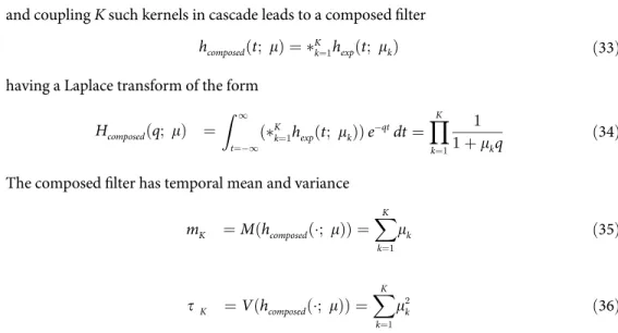
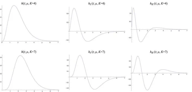
Fig. 4shows graphs of these kernels for two combinations ofμandKthat correspond to the same value of the composed varianceτ=Kμ2. Notably, these kernels are highly asymmetric for small values ofK, whereas they become gradually more symmetric asKincreases. Figs.5–6

show corresponding compositions of truncated exponential kernels for self-similar distribu-tions of the intermediate time constants according to Equadistribu-tions (38), (39) and (40) forc¼ ffiffiffi

2

p

andc= 23/4. Comparingfig. 4andfigs.5–6, the use of a self-similar distribution of the time constants (infigs.5–6) allows for smoother behaviour near the origin with increasingKwhile not increasing the temporal delay as much as for the kernels corresponding to a uniform distri-bution of the intermediate temporal scale levels (infig. 4).

Time-recursive computation of temporal derivatives. Temporal scale-space derivatives

of orderrcan be defined from this scale-space model according to

Ltrð; tKÞ ¼@_trLð; t_KÞ ¼ ð@_trðK_k¼1hexpðt; mkÞÞ f ð47Þ

Fig 4.Equivalent kernelshcomposedðt; mÞ ¼ K

k¼1hexpðt; mÞwith temporal varianceτ= 1corresponding to the composition of K truncated exponential

kernels with equal time constantsμand their first- and second-order derivatives.(top row)k= 4 andm¼ ffiffiffiffiffiffiffiffi

1=4

p

. (bottom row)k= 7 andm¼ ffiffiffiffiffiffiffiffi

1=7

p

Fig 6.Equivalent kernelshcomposedðt; mÞ ¼ K

k¼1hexpðt; mkÞwith temporal varianceτ= 1corresponding to the composition of K= 4or K= 7truncated

exponential kernels with different time constants defined from a self-similar distribution of the temporal scale levelsaccording to Equations (38), (39) and (40) and corresponding to a uniform distribution in terms of effective temporal scaleτ_eff= logτforc= 23/4and with their first- and

second-order derivatives.

doi:10.1371/journal.pone.0119032.g006

Fig 5.Equivalent kernelshcomposedðt; mÞ ¼ K

k¼1hexpðt; mkÞwith temporal varianceτ= 1corresponding to the composition of K= 4or K= 7truncated

exponential kernels with different time constants defined from a self-similar distribution of the temporal scale levelsaccording to Equations (38), (39) and (40) and corresponding to a uniform distribution in terms of effective temporal scaleτeff= logτforc¼

ffiffiffi

2

p

and with their first- and second-order derivatives.

where the Laplace transform of the composed (equivalent) derivative kernel is

HcomposedððrÞ q; t_{KÞ ¼}qrY K

k¼1 1

1_þm_kq ð48Þ

For this kernel to have a net integration effect (to enable well-posed derivative operators), the total order of differentiation must not exceed the total order of integration. Thereby,r<kis a necessary requirement. The composed transfer function must havefiniteL2-norm.

A very useful observation that can be made concerning derivative computations is that tem-poral derivatives can equivalently be computed from differences between different temtem-poral channels. Let us first assume that all time constantsμiare different in (48). Then, a partial

frac-tion division gives

HcomposedðrÞ ðq; tkÞ ¼

Xk

i¼1

AiHprimðq; miÞ ð49Þ

where

Ai ¼ ð 1Þr

mr i

Yk

j¼1;j6¼i

1

ð1 m_j=m_iÞ ð1ikÞ ð50Þ

showing thateach temporal derivative can be computed as a linear combination of the represen-tations at the different time-scales.

More realistically, the channels that we can regard as available at a certain temporal scale with indexkwill not be the results of direct filtering with different time constantsμi. Rather,

we would like to use the intermediate outputs from the cascade coupled recursive filtersH compo-sed(q;τi) fork−rik. Decomposition ofHð

rÞ

composedinto a sum ofrsuch transfer functions

HcomposedðrÞ ðq; tkÞ ¼

Xk

i¼k r

BiHcomposedðq; tiÞ ð51Þ

shows that the weightsBiare given as the solution of a triangular system of equations provided

that the necessary conditionr<kis satisfied

ð 1_Þr

mr i

Yk

j¼iþ1 1

ð1 m_j=miÞ¼Biþ

Xk

n¼iþ1 Bn

Yn

j¼iþ1 1

ð1 m_j=miÞ ðk rikÞ: ð52Þ

It can be shown that the Laplace transforms of the equivalent derivative computation kernels satisfy the following recurrence relation (Lindeberg and Fagerström [44])

HcomposedðrÞ ðq; tkÞ ¼

1

m_k H

ðr 1Þ

composedðq; tk 1Þ H ðr 1Þ

composedðq; t_kÞ

ð53Þ

Multi-scale spectrograms for auditory signals

The above treatment concerning is general and can be used for modelling desirable properties of temporal receptive fields for a variety of time-dependent sensory signals. For auditory sig-nals, an additional structural requirement arises from the fact that the auditory information is transferred in terms of sound waves that travel from the transmitter to the receiver and the au-ditory information can be encoded in terms of oscillation frequencies of the air pressure that generates the sensory signal. For this reason and from our knowledge that the variations due to the geometry and other properties of the cochlea leads to physical resonances whose effect can be modelled as a physical Fourier transform,spectrogramsare a common tool for analyzing auditory information.

Note that our primary aim is not to specifically model, for example, the measured response of the nerves coming from the cochlea as typically done in previous auditory models (Patterson et al. [36]). Instead we are following the scale-space theory using the principle of invariance as outlined in the sections“Structural requirements on temporal receptive fields”and “Scale-space concepts for purely temporal domains”.

Based on the two models for temporal receptive fields (non-causal in the section “Non-caus-al Gaussian tempor“Non-caus-al sc“Non-caus-ale-space”and time-causal in the section“Time-causal temporal scale-space”), we can use the temporal smoothing functions in these two temporal scale-space mod-els as scale-dependent window functions for defining two types of complex-valuedmulti-scale spectrogramsaccording to

Sgðt;o; t_{Þ ¼}

Z 1

t0_{¼ 1}

gðt t0_{; tÞfðt}0_Þe iot0

dt0 _ð54Þ

Shðt;o; mÞ ¼

Z 1

t0_{¼ 1}hcomposedðt t

0_{; mÞfðt}0_Þe iot0_dt0 _ð55Þ

where

• g(t;τ) is a temporal Gaussian kernel of the form (26),

• hcomposed(t;μ) withμ= (μ1,. . .,μK) is the equivalent convolution kernel corresponding to a

cascade of truncated exponential filters of the form (33).

This implies that the convolution kernels in the temporal scale-spaces for a general time-vary-ing signal are used as scale-dependent window functions for defintime-vary-ing windowed Fourier trans-forms of different temporal extent.

For a given value ofτ, the spectrogram becomes a 2-D function. With the definition extend-ed to all values ofτ, the spectrogram based on Gaussian window functions instead becomes a 3-D volume over all temporal extents of the window function or alternatively a set of discrete 2-D slices for the window functions based on truncated exponential functions coupled in cas-cade for vectorsμ= (μ1,. . .,μK) of different lengthK.

related to a windowed Fourier transform at any finer scale using thecascade property

Sð;o; t2Þ ¼ wð; t2 t1Þ Sð;o; t1Þ; ð56Þ

Sð;o; t_{nÞ ¼ ð}DwÞð; m7!nÞ Sð;o; t_mÞ: ð57Þ

derived from the semi-group structure (15) or the Markov property (18) of the underlying scale-space kernels. Combined with the additional scale-space properties of non-creation of new structures with increasing scale, this guarantees well-founded theoretical properties be-tween corresponding windowed Fourier transforms at different temporal scales.

In most other work on auditory signal processing, there is often an implicit assumption that one chooses a scale for computing the auditory features that seems to work and on which later stage analysis is then based. By the presented formulation of multi-scale spectrograms, we aim at making the consequences of such assumptions explicit, and emphasizing the possibility of computing auditory features at multiple temporal scales as an integrated part of the analysis. Compared to the more traditional approach of computing spectrograms from local fast Fourier transforms combined with local windowing operations, this formulation of multi-scale spectro-grams also avoids the concatenation of such windowing operations altogether and thereby the artifacts caused by these.

The scale-space approach for defining multi-scale auditory spectrograms implies that in-stead of computing a scale-space representation of the original auditory signal, the auditory sig-nal is first projected onto the two orthogosig-nal dimensions cosωtandisinωtof a complex sine wavee−iωt

fcosðt;oÞ ¼fðtÞ cosot fsinðt;oÞ ¼fðtÞsinot ð58Þ

for which temporal scale-space representations are then defined, implying that the multi-scale spectrogram can be seen as a complex-valued scale-space transform.

Invariance and covariance properties. Concerning the symmetry requirements of a

general temporal sensory front-end described in the section“Structural requirements on temporal receptivefields”, the linearity of the scale-space operations is transferred to a linearity in the complex multi-scale spectrograms (54)–(55). This implies that multiple sources of sound will be combined in an additive manner in terms of their complex-valued responses and that sound sources of different strength (sound pressure) will be handled in a similar manner up to a multiplication of the strength of the signal.

Regarding temporal shift invariance, the magnitude mapsjSgjandjShjare invariant under a

shift of the temporal axis, whereas the phase of the truly complex spectrogramsSgandShwill

be transformed in a predictable manner between similar sound signals at different time mo-ments or from different distances to the observer.

Under a local rescaling of the temporal axis

t7!at ð59Þ

the temporal receptivefields from the Gaussian scale-space model are fully scale covariant and the corresponding complex-valued multi-scale spectrograms are transformed according to

Sðt;o; t_{Þ 7!}S at;o

a; a

2_t

: ð60Þ

If we let the window scales¼ ffiffiffiffi

t p

corresponding frequency shift

o_7!o

a: ð61Þ

If the temporal window functions on the other hand do not have the temporal extent propor-tional to the wavelength, then temporal covariance does not hold within the same 2-D slice but still holds within the 3-D multi-scale spectrogram based on Gaussian window functions be-cause of their self-similarity over scale, whereas the corresponding scaling relations can only be approximate for the truncated exponential functions coupled in cascade, because of the tempo-ral scale levels being restricted to a discrete set of values.

Again there may not be any principled reason for preferring a particular temporal scale over another. The multi-scale nature of these spectrograms makes this aspect explicit and opens up for using different temporal scales for different auditory tasks, where different temporal scales may have complementary advantages.

Relations to Gabor functions. By rewriting the expression (54) for the complex-valued

spectrogram based on the Gaussian temporal scale-space concept as

Sgðo;t; t_{Þ ¼e} iot

Z 1

t0_{¼ 1}gðt t

0_{; tÞe}ioðt t0Þ_fðt0_Þdt0_{; ð62Þ}

it can be seen that up to a phase shift, this multi-scale spectrogram can equivalently be inter-preted as the convolution of the original auditory signalfbyGabor functions[28] of the form

Gðt;o; tÞ ¼gðt; tÞeiot_{: ð63Þ}

Such Gabor functions have been previously used for analyzing auditory signals by several au-thors, including (Wolfe et al. [29]; Kleinschmidt et al. [49,50]; Lobo and Loizou [30]; Qiu et al. [31]; van de Boogart and Lienhart [51]; Ezzat et al. [52]; Domont et al. [53]; He et al. [54]; Heckmann et al. [55]; Wu et al. [32]; Schädler et al. [56]; Sameh and Lachiri [57]). Our theory provides a new way of deriving this representation with special emphasis on the multi-scale na-ture of the Gaussian window functions and their resulting cascade properties between spectro-grams at different temporal scales.

Relations to Gammatone filters. In the special case when the time constants of all theK

truncated exponential filters that are coupled in cascade are all equalμk=μ, it follows from

combination of Equations (55) and (44) that the multi-scale spectrogram is given by

Shðt;o; m;KÞ ¼e iot

Z 1

t0_{¼ 1}

ðt t0_ÞK 1 e ðt t0_Þ=m

mK_GðKÞ e

ioðt t0Þ_fðt0_Þdt0 _ð64Þ

and does up to a phase shift correspond to convolution of the input signalfbyfilters of the form

hcosðt;o; m;KÞ ¼ t K 1_e t=m

mK_GðKÞ cosot; ð65Þ

hsinðt;o; m;KÞ ¼ t K 1_e t=m

mK_GðKÞ sinot: ð66Þ

For comparison, theGammatonefilterwith parametersaandband frequencyϕis defined ac-cording to

By identification of the parameters

a¼ 1

mK_GðKÞ b¼

1

2pm ð68Þ

and usingω= 2π ϕit follows that we can derive the Gammatonefilter as a special case of applying a time-causal scale-space representation with discrete scale levels to the projections fcos(t,ω) andfsin(t,ω) of an auditory signalf(t) onto a complex sine wavee−iωt.

Gammatone filter banks are also commonly used in audio processing (Johannesma [33]; Patterson et al. [34,36]; Hewitt and Meddis [35]; Irino and Patterson [58]; Ambikairajah [59]; Hohmann [60]; van Immerseel and Peeters [61]; Schlute et al. [62]; Ngamkham et al. [63]). The present treatment provides a new way of deriving them in a principled and conceptually similar way as the Gabor filters can be derived, with the differences that the temporal filtering operations are required to be truly time-causal and that only a discrete set of temporal scale lev-els is to be used.

Generalized Gammatone filters. In addition, by allowing for different time constants in

the primitive truncated exponential filters, this scale-space concept leads togeneralized Gam-matone filters

hcosðt;o; m_{Þ ¼} hcomposedðt; m_Þcosot _ð69Þ

hsinðt;o; mÞ ¼ hcomposedðt; mÞsinot ð70Þ

withhcomposedaccording to (34). By comparing graphs of the two classes of auditory receptive

fields based on time-causal window functions (Lindeberg and Friberg [64],fig. 6), it can be seen that the frequency selectivefilters based on truncated exponentialfilters having a logarith-mic distribution of the intermediate temporal scale levels allow for a faster temporal response compared to the correspondingfilters based on truncated exponentialfilters with equal time constants. Thereby, these generalized Gammatonefilters allow for additional degrees of free-dom to obtain different trade-offs between the frequency selectivity and the temporal delay of time-causal window functions by varying the number of levelsKand the distribution parame-terc—see the appendices“Frequency selectivity of the spectrograms”and“Temporal dynamics of the time-causal kernels”for an in-depth analysis of the frequency selectivity and the tempo-ral delay of such kernels.

Figs.7–8show spectrograms computed in this way for two sound signals using the three differ-ent types of temporal window functions and using fixedvs. frequency-dependent window scales.

Frequency-dependent window scale. To guarantee basic covariance properties of the

spectrogram under a frequency shift

o7!a o ð71Þ

it is as earlier mentioned natural to let the temporal window scale vary with the frequencyωin such a a way that the temporal window scale in units ofs¼ ffiffiffiffi

t p

isproportional to the wave-lengthλ= 2π/ω

t_¼ 2pn

o

2

ð72Þ

Fig 7.Spectrograms with a fixed temporal window scalest¼

ffiffiffiffi t

p

corresponding spectrogram should appear similar while shifted by one octave, if the frequency axis of the spectrogram is parameterized on a logarithmic scale.

To prevent the temporal window scale from being too short for high frequency sounds, we have additionally chosen to add asoft lower boundsuch that the temporal extent is instead cho-sen according to

t_¼t_0þ 2pn

o

2

ð73Þ

wheret_0¼s2

0denotes a lower bound on the temporal window scale. Thereby, frequency co-variance of a 2-D spectrogram will only be approximate, while being a good approximation ifτ

τ0. If we quantifyττ0asτ=β2τ0, then the soft lower bound corresponds to

o¼ ffiffiffiffiffiffiffiffiffiffiffiffiffi2pn

b2 1 p

s₀ ð74Þ

which withσ0= 1 ms,n= 8 andβ= 2 corresponds to a frequency of about 4 600 Hz. By varying

the parametersσ0andn, we can move the frequency where deviations from true invariance

begin to occur for a given value of the tolerance parameterβ.

To prevent the temporal delay from being too long at low frequencies, one can also intro-duce asoft upper bound on the temporal scale

t0_¼ t

1_þ t

t₁

p 1=p

ð75Þ

for suitable values ofτ1andp. Then, approximate frequency covariance will hold over some subset of frequencies defined by the parametersn,τ0,τ1andp.

In human hearing, there is different evidence that the resolution of pitch perception is the highest in the area around 0.6-2 kHz and then decreases for both lower and higher frequencies (see e.g. Hartmann [65]; Moore [66]). Furthermore, within the middle area 0.6-2 kHz the rela-tive pitch sensitivity appears to be approximately constant. The synchrony in the neural firing in the auditory nerve decreases with increasing frequency (Johnson [67]). The ability to identi-fy the pitch of a mistuned harmonic decreases with increasing frequency exhibiting a knee at around 2 kHz (Hartmann et al. [68]). A lower frequency boundary can also be motivated from the size of the critical bands which according to the classic Zwicker data changes from being proportionally constant (about a musical minor third) for frequencies above 500 Hz to being constant (about 100 Hz) for frequencies below 500 Hz (Zwicker [69]). More recent data exhibit a similar but less strong tendency (Moore [70], page 77). Thus, in summary, there should pre-sumable be both an upper and a lower limit for self-similarity.

Receptive fields defined over the spectrogram

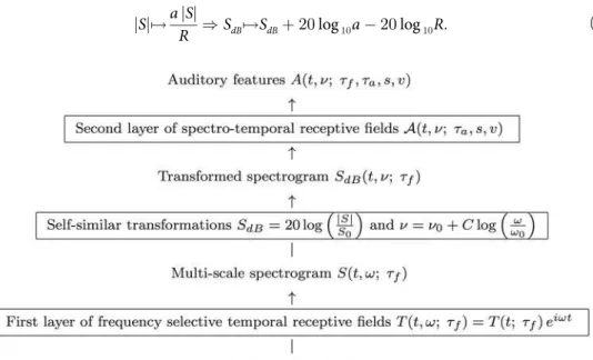
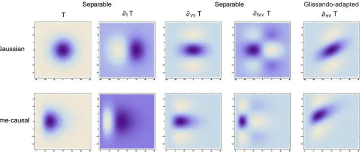
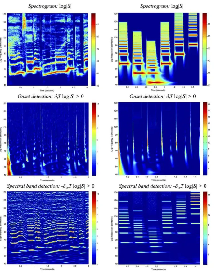
Given that a spectrogram has been computed by a first layer of auditory receptive fields, we de-fine asecond layer of receptive fieldsby operating on the spectrogram with 2-D spectro-tempo-ral filters (seefig. 9) in a structurally similar way as visual receptive fields are applied to time-varying visual input (Lindeberg [5,27]).

distribution of the temporal scale levels withc¼ ffiffiffi

2

p

.The vertical axis shows the logarithmic frequency expressed in semitones with 69 corresponding to the tone A4 (440 Hz). Notice that while the different types of spectrograms largely capture similar types of spectro-temporal structures, there is a significant difference in temporal delay and temporal response characteristics between the non-causal and the time-causal spectrograms.

Fig 8.Spectrograms with the temporal window scale proportional to the wavelength according toEquation (73)forn= 8 and a soft lower thresholds0¼

ffiffiffiffiffiffi t0

Logarithmic transformations of the spectrogram

Prior to the definition of receptive fields from the spectrogram, it is natural to allow for a self-similarlogarithmic transformation of the magnitude values

SdB¼20log10

jSj

S0

: _ð76Þ

A logarithmic transformation of the magnitude of the spectrogram implies that a multiplicative transformation of the sound pressuref7!a f, corresponding tojSj 7!ajSj, or an inversely pro-portional reduction in the sound pressure of the signal from a single auditory point source as function of distancef7!f/R, corresponding tojSj 7! jSj/R, are both transformed into a subtrac-tion of the logarithmic magnitude by a constant

jSj7!ajSj

R )SdB7!SdBþ20log10a 20log10R: ð77Þ levels and (bottom row) a cascade of seven time-causal recursive filters having a logarithmic distribution of the temporal scale levels withc¼ ffiffiffi

2

p .

The vertical axis shows the logarithmic frequency expressed in semitones with 69 corresponding to the tone A4 (440 Hz). The spectrograms computed with time-causal kernels have been delay compensated by a temporal delay defined from the position of the first inflection point of the temporal window function. Notice that while the different types of spectrograms to some extent capture qualitatively similar types of spectro-temporal structures, there is a significant difference in temporal delay and temporal response characteristics between the non-causal and the time-causal spectrograms. Compared to the

spectrograms infig. 7that are computed with a fixed temporal scale implying that the spectral bands become more narrow at higher frequencies, the use of a temporal scale proportional to the wavelength specifically implies that the widths of the spectral bands are here much more uniform over frequencies (see the section“Frequency selectivity of the spectrogram”for a theoretical analysis).

doi:10.1371/journal.pone.0119032.g008

Fig 9.Schematic illustration of the definition of auditory features from a second layer of receptive fields over the spectrogram, where we also allow for a logarithmic transformation of the magnitude values_jS_jof the spectrogram prior to the application of the second layer of linear receptive fields and

make use of a logarithmic transformation of the frequenciesn_¼n0þClog ðo0o

Þbefore defining the linear receptive fields over the spectro-temporal domain.Regarding the scale parameters, the first layer of temporal receptive fields depends on a single temporal scale parameterτffor the frequency selective

temporal filters, whereas the second layer of auditory receptive fields also depends on an additional temporal scale parameterτa, a logspectral scale parametersover the logarithmic frequenciesνand a glissando

If we operate on the logarithmically transformed spectrogram by a receptivefieldA_Sthat is based on a combination of a spectro-temporal smoothing operationT_Swith logspectral and temporal scale parameters as determined by a spectro-temporal covariance matrixS, temporal and/or logspectral derivatives@tα_νβof ordersαandβwith at least one ofα>0 orβ>0

A

SSdB¼@ta_nbT_SS_dB ð78Þ

then it follows that the influence on the receptivefield responses of the constantsaandR

A

SSdB ¼ @ta_nbT_SðS_dBþ20log10a 20log10RÞ

¼ @ta_nbT_SS_dBþ0þ0

ð79Þ

will be eliminated by the derivative operation if the constantsaandRdo not depend on timet or the logarithmic frequencyν, implyinginvariance of the second-layer receptivefield responses to variations in the sound pressure or the distance to a sound source.

A logarithmic transformation of the magnitude is compatible with theWeber-Fechner law, stating that the ratio of an increment thresholdΔIof a stimulus for a just noticeable different relative to the background intensityIis constant over large ranges of magnitude variations, which approximately holds in both visual and auditory perception (Palmer [71]; Kandel et al. [72]).

Furthermore, since logarithmic frequencies constitute a natural metric for relating frequen-cies of sound (Fletscher [73]; Kandel et al. [72]; Young [74]) and there is an approximately log-arithmic distribution of frequencies both on the basilar membrane (Greenwood [75]) and in the organization of the auditory cortex (Romani et al. [76]), it is natural to express these de-rived receptive fields in terms oflogarithmic frequencies

n_¼n_0þC log o

o0

ð80Þ

for some constantsCandω0, where specificallyν0= 69,C= 12/log2 andω0= 2π440

corre-spond to logarithmic frequencies according to the MIDI standard.

This logarithmic parameterization of frequency implies that a shift in frequency, caused by e.g. transposing a piece of music by one octave, or varying the fundamental frequency in sing-ing resultsing-ing in a multiplicative transformation of the harmonics (overtones), correspond to a meretranslationin logarithmic frequency.

Structural requirements on second-layer receptive fields

Given a transformed spectrogram defined in this way, let us define a family of second layer spectro-temporal receptive fieldsA(t,ω;S) that are to operate on the transformed spectrogram SdB(t,ν;τ) and be parameterized by some multi-dimensional spectro-temporal scale parameter Sthat includes smoothing over timetand logarithmic frequenciesν, and for which the corre-sponding operatorA_Sis required to obey:

(i) linearityover the logarithmic spectrogram

A_Sða S1þb S2Þ ¼aA_SðS1Þ þbA_SðS2Þ ð81Þ

spectrograms as defined by spectro-temporal smoothing kernels do also transfer to spectro-temporal derivatives of these,

(ii) shift-invariancewith respect to translations over timet7!t+Δtand logarithmic fre-quenciesν7!ν+Δν

A_SðS_ðDt;DnÞSÞ ¼S_ðDt;DnÞðA_SSÞ ð82Þ

such that all temporal moments and all logarithmic frequencies are treated in a similar manner. Temporal shift invariance implies that an auditory stimulus should be per-ceived in a similar manner irrespective of when it occurs. Shift-invariance in the loga-rithmic frequency domain implies that, for example, a piece of music should be perceived in a similar manner if it is transposed bye.g. one octave.

These conditions together imply that the spectro-temporal receptive fields should be given by convolution with some two-dimensional kernel over the spectro-temporal domain (Hirsch-mann and Widder [41]):

ðA_SSdBÞðt;n; t_f;SÞ ¼

Z 1

x¼ 1 Z 1

Z¼ 1

Tðx;Z; SÞSdBðt x;n Z; t_fÞdxdZ: ð83Þ

To characterize what types of receptivefields are compatible with scale-space properties, we will next impose additional structural requirements, which will take different forms depending on whether the temporal dimension is treated in a time-causal or non-causal manner:

Relations between receptive fields at different spectro-temporal scales. For

pre-re-corded sound signals, for which we can take the freedom of accessing data from the virtual fu-ture in relation to any time moment, we impose a

(iii.a) continuous semi-group structure over spectro-temporal scales on the second layer re-ceptive fields

Tð;; S2Þ ¼Tð;; S2 S1Þ Tð;; S1Þ ð84Þ corresponding to an additive structure over the multi-dimensional scale parameterS.

For time-causal signals, we require:

(iii.b) a continuous semi-group structure over logspectral scaless

Tð; s2Þ ¼Tð; s2 s1Þ Tð; s1Þ ð85Þ

and a Markov property between adjacent temporal scales

Tð; t_kþ1Þ ¼ ðDTÞð; kÞ Tð; tkÞ: ð86Þ These requirements are analogous to the previous treatment in the section“Structural require-ments on temporal receptive fields”, with extensions from a purely temporal domain to a spec-tro-temporal domain.

Non-creation of new spectro-temporal structures with increasing scale. When

temporal dimension is treated in a time-causal or non-causal manner, we formalize this condi-tion as:

(iv.a) For the non-causal Gaussian spectrogram (54), for which temporal causality of the temporal smoothing kernels is disregarded, we requirenon-enhancement of local ex-tremain the sense that if for some scaleS0the point (t0,ν0) is a local maximum

(mini-mum) for the mapping (t,ν)7!(A_SSdB)(t,ν;S0) then the value at this point must not

increase (decrease) with increasing scaleS.

(iv.b) For the time-causal spectrogram (55) based on truncated exponential filters coupled in cascade (33), we require: (iv.b1) the smoothing operation over the logspectral do-main to satisfy non-enhancement of local extrema in the sense that if at some logspec-tral scales0a pointν0is a local maximum (minimum) of the mappingν7!(ASSdB)(ν;

s0) obtained by disregarding the temporal variations, then the value at this point must

not increase (decrease) with increasing logspectral scales, and (iv.b2) the smoothing operation over time to be a time-causal scale-space kernel guaranteeing non-creation of new local extrema under an increase of the temporal scale parameterτ.

Glissando covariance. In musical performance, the frequencies may vary continuously

over time in such a way that the fundamental frequencyω1and the harmonics (overtones)ωj

are all multiplied by the same time-varying factorωj(t) =ψ(t)ωj. This is in particular prominent

in singing, but may occur in all instruments with continuous pitch control. In terms of loga-rithmic frequencies, we can model a local linearization of this temporal variability as aglissando transformationof the form

n_ðtÞ ¼n_0þv t ð87Þ

analogous to the way spatial image data may be subject to local Galilean transformations over time. Comparing two spectrograms, one with constant frequencies over time and one with line-arly varying logarithmic frequencies, the glissando transformation can be expressed in operator form as

S0_¼G

vS corresponding to S0ðt;n0Þ ¼Sðt;nÞ ð88Þ

forν0_{=ν+v t. In relation to receptivefield responses that are computed over the two domains} with spectro-temporal scale parametersSandS0_{, we may require:}

(v) If two local patches of two spectrograms are related by a local glissando transforma-tion, then it should be possible to relate the local spectro-temporal receptive field re-sponses such that

A_G

vðSÞGvS¼GvASS ð89Þ for some transformationS0_=G

v(S) of the spectro-temporal scale parametersS.

Idealized models for spectro-temporal receptive fields