Sky cover from MFRSR observations: cumulus clouds

(1)

AMTD

4, 715–735, 2011

Sky cover from MFRSR observations: cumulus clouds

E. Kassianov et al.

Title Page

Abstract Introduction

Conclusions References

Tables Figures

◭ ◮

Back Close

Full Screen / Esc

Printer-friendly Version Interactive Discussion

Discussion

P

a

per

|

Dis

cussion

P

a

per

|

Discussion

P

a

per

|

Discussio

n

P

a

per

Atmos. Meas. Tech. Discuss., 4, 715–735, 2011 www.atmos-meas-tech-discuss.net/4/715/2011/ doi:10.5194/amtd-4-715-2011

Atmospheric Measurement Techniques Discussions

This discussion paper is/has been under review for the journal Atmospheric Measure-ment Techniques (AMT). Please refer to the corresponding final paper in AMT

if available.

Sky cover from MFRSR observations:

cumulus clouds

E. Kassianov, J. Barnard, L. K. Berg, C. Flynn, and C. N. Long

Pacific Northwest National Laboratory, Richland, Washington, 99352, USA

Received: 28 December 2010 – Accepted: 18 January 2011 – Published: 24 January 2011 Correspondence to: E. Kassianov (evgueni.kassianov@pnl.gov)

(2)

AMTD

4, 715–735, 2011

E. Kassianov et al.

Title Page

Tables Figures

◭ ◮

Back Close

Full Screen / Esc

Discussion

P

a

per

|

Dis

cussion

P

a

per

|

Discussion

P

a

per

|

Discussio

n

P

a

per

|

Abstract

The diffuse all-sky surface irradiances measured at two nearby wavelengths in the visi-ble spectral range and their model clear-sky counterparts are two main components of a new method for estimating the fractional sky cover of different cloud types, including cumulus clouds. The performance of this method is illustrated using 1-min resolu-5

tion data from ground-based Multi-Filter Rotating Shadowband Radiometer (MFRSR). The MFRSR data are collected at the US Department of Energy Atmospheric Radi-ation Measurement (ARM) Climate Research Facility (ACRF) Southern Great Plains (SGP) site during the summer of 2007 and represent 13 days with cumulus clouds. Good agreement is obtained between estimated values of the fractional sky cover and 10

those provided by a well-established independent method based on broadband obser-vations.

1 Introduction

Cloud fraction (CF) is a key cloud property that controls the amount of transmitted and reflected solar radiation, and thus the radiation balance at the surface (e.g., Dong et al., 15

2006; Berg et al., 2010). Aerosols may change substantially the CF, and these changes are thought to be sensitive to the aerosol optical depth (AOD) and the single-scattering albedo (SSA) (Perlwitz and Miller, 2010). The strength and even sign of the CF-AOD relationship have been controversial for at least a decade (e.g., Quaas et al., 2010, and references therein) and such controversy has resulted partially from sampling issues. 20

For example, the aerosol and cloud properties of interest are obtained typically with different spatial/temporal resolution by several different surface and space born instru-ments. Thus, there is an essential need to have a tool that can o_ffer the coincident and collocated measurements and retrievals of cloud and aerosol properties.

Recently, Kaufman and Koren (2006) applied data from the Aerosol Robotic Net-25

(3)

AMTD

4, 715–735, 2011

E. Kassianov et al.

Title Page

Tables Figures

◭ ◮

Back Close

Full Screen / Esc

Discussion

P

a

per

|

Dis

cussion

P

a

per

|

Discussion

P

a

per

|

Discussio

n

P

a

per

directional CF, defined as a fraction of time that a ground-based sunphotometer would detect a cloud for a given direction from the instrument to the sun. The data were col-lected around the globe and subdivided into continental, coastal/oceanic, and biomass burning subsets. They found an increase in the directional CF of water clouds with an increase in AOD and decrease of the aerosol absorption, and also demonstrated that 5

this relationship is not a function of aerosol type and location.

The majority of the climate-related studies (e.g., Zhang et al., 2010) have used the fractional sky cover N, which is a hemispherical measure of cloud amount. The es-timation of N can be performed using empirical methods N can be performed using empirical methods. One of them (Long et al., 2006) applies measured shortwave, 10

broadband all-sky fluxes and their inferred clear-sky counterparts. Here we illustrate how spectrally resolved fluxes in the visible spectral range can be applied for estimat-ingN. Since cumulus clouds appear to be more susceptible to the aerosol changes in comparison with other low clouds (Su et al., 2010), this estimation is illustrated for days with cumulus clouds and typical aerosol loading. For these selected days, the aerosol 15

optical properties (e.g., AOD and SSA) are consistent with the climatological values (e.g., McComiskey et al., 2008; Michalsky et al., 2010).

2 Approach

We select 13 days with cumulus clouds observed during summer 2007 at the US De-partment of Energy Atmospheric Radiation Measurement (ARM) Climate Research 20

Facility (ACRF) Southern Great Plains (SGP) site following the method described by Berg and Kassianov (2008). The site is equipped with numerous instruments for sam-pling cloud, aerosol and radiative properties. In particular, the ARM Active Remotely Sensed Clouds Locations (ARSCL) value-added product combines measurements of the cloud radar, laser ceilometers, microwave radiometer and micropulse lidar, and the 25

(4)

AMTD

4, 715–735, 2011

E. Kassianov et al.

Title Page

Tables Figures

◭ ◮

Back Close

Full Screen / Esc

Discussion

P

a

per

|

Dis

cussion

P

a

per

|

Discussion

P

a

per

|

Discussio

n

P

a

per

|

Thus, the ASRCL-based cloud properties (e.g., cloud fraction) may not be represen-tative of those obtained for a region surrounding these instruments. In our analysis, we use the ASRCL-based cloud fraction and cloud base heights (CBH). In addition to the ARSCL measurements, we apply collocated and coincident observations of the total sky imager (TSI). The TSI has a hemispherical FOV and routinely provides time series 5

of hemispherical sky images for a large area neighboring the ACRF site.

The Multi-Filter Rotating Shadowband Radiometers (MFRSRs) measure the total all-sky surface downwelling irradiance and its diffuse and direct components at six narrowbands centered at wavelengths of 415, 500, 615, 673, 870, and 940 nm (visible spectral region) with 1-min temporal resolution (Harrison and Michalsky, 1994). The 10

high-temporal resolution MFRSR observations at the ACRF site allow one to capture the small-scale cloud-induced fluctuations of optical depth (Fig. 1a): instances with “spikes” in the optical depth define events when a cloud blocks the direct solar beam and the nominal optical depth is a sum of AOD and cloud optical depth (COD). The observed large sharp changes of the diffuse irradiance (Fig. 1b) from smooth to rough 15

are due to clouds, and changes of their geometrical and optical properties.

Originally, Min et al. (2008) suggested a technique forNestimating from the MFRSR data. This technique involves the ratio of MFRSR-measured diffuse transmittance at two wavelengths (870 and 415 nm), the so-called the transmittance ratio. The diffuse transmittance was defined as a di_ffuse flux divided by the corresponding solar constant 20

inferred from Langley regression on sky days. The technique requires the clear-and cloudy-sky baselines. To obtain them, sufficiently long periods with optically thick clouds are required. Such periods can be obtained easily for clouds with large horizon-tal extent such as stratus/stratocumulus clouds. On the other hand, cumulus clouds may be optically thin and have more limited spatial extent. The corresponding cloudy-25

(5)

AMTD

4, 715–735, 2011

E. Kassianov et al.

Title Page

Tables Figures

◭ ◮

Back Close

Full Screen / Esc

Discussion

P

a

per

|

Dis

cussion

P

a

per

|

Discussion

P

a

per

|

Discussio

n

P

a

per

diurnal AOD variations where “evening” AOD values (from 17:00 to 18:00 CST) exceed their “morning” counterparts (from 09:00 to 10:00 CST) more than two times (Fig. 1a). As a result, the obtained “morning” clear-sky baseline is not representative for the “evening” period (Fig. 1c) and vice versa.

For a given solar zenith angle, the temporal variations of the clear-sky fluxes are 5

mostly governed by changes of aerosol properties, thus, these changes should be considered. We apply a three-step physically-based approach (Kassianov et al., 2010) utilizing (i) the spectrally resolved direct and diffuse irradiances for retrieval of aerosol optical properties during clear sky periods (Harrison and Michalsky, 1994; Kassianov et al., 2007), (ii) temporal interpolation of the retrieved clear-sky aerosol properties for 10

temporally “nearby” cloudy intervals, and (iii) calculations the clear-sky fluxes by using a radiative transfer model and the obtained aerosol properties as input. By “nearby” we mean cloudy periods, during which we cannot find aerosol optical properties. These periods are sandwiched between clear periods, when it is possible to obtain aerosol optical properties. These properties include the AOD, SSA and asymmetry parameter. 15

Figure 1c shows an application of this approach for obtaining a “clear-sky” baseline for the di_fference of the measured di_ffuse all-sky fluxes at two wavelengths (415 and 500 nm). We apply this difference to defineN as follows.

In the framework of plane-parallel approximation, all-sky diffuse fluxes can be de-scribed as

20

F(λ)=(1−N)F0(λ)+NF1(λ), (1)

whereF0 and F1 is the clear-sky and cloudy-sky diffuse flux, respectively. Obviously,

this approximation is not able to explain the large fluctuations of the observed diffuse fluxes (Fig. 1b). Note that these fluctuations are strongly correlated at 415 and 500 nm wavelengths (Fig. 1b). Consequently, the cloud-induced contribution to the all-sky dif-25

(6)

AMTD

4, 715–735, 2011

E. Kassianov et al.

Title Page

Tables Figures

◭ ◮

Back Close

Full Screen / Esc

Discussion

P

a

per

|

Dis

cussion

P

a

per

|

Discussion

P

a

per

|

Discussio

n

P

a

per

|

spectral diffuse fluxes (415 and 500 nm), this difference is less sensitive to the cloud-induced e_ffects. Thus, for estimating N we apply the di_fference that can be written as

F(500)−F(415)=(1−N)F0(500)−F0(415)

+N[F1(500)−F1(415)] (2a)

The right part of Eq. (2a) has two terms, which representN-weighted contributions 5

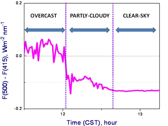
of the clear-sky and cloudy-sky to the difference of diffuse fluxes. For a given sky cover (N), the sign and magnitude of these contributions are defined by spectral changes of the solar constant, cloud and aerosol properties and surface albedo. Analysis of time series of the TSI images and the MFRSR-measured diffuse irradiances reveals that the observed differenceF(500)−F(415) has positive and negative values for the

com-10

pletely overcast cloudy (N=1) and clear-sky (N=0) conditions, respectively (Fig. 2). Thus, the corresponding sign change in this difference can be considered as a sim-ple indicator of switching from a partly-cloudy sky to overcast sky. Also, this analysis reveals that the largest positive values occur for optically thin clouds (cloud images are bright) while the smallest positive values observed for optically thick clouds (cloud 15

images are dark).

Figure 2 shows the difference obtained for a day when the sky was almost com-pletely overcast with optically thin clouds around noon. The corresponding average value of the overcast difference F1(500)−F1(415) is about 0.03. A well-known weak

spectral dependence of cloud optical properties in the visible spectral range is mainly 20

responsible for the small values of the overcast difference. In contrast, a strong spec-tral dependence of the aerosol optical properties (e.g., AOD) in the visible specspec-tral range is mainly responsible for the relatively large values of the clear-sky difference

F0(500)−F0(415). From Fig. 2 one can conclude that the overcast value (0.03) is about

four times smaller than absolute value of its clear-sky counterpart (0.13). Note that the 25

latter demonstrates small day-to-day variations. For time periods with optically thick clouds, the overcast di_fference is even smaller (about 0.01). Thus, this value (∼0.01) is

(7)

AMTD

4, 715–735, 2011

E. Kassianov et al.

Title Page

Tables Figures

◭ ◮

Back Close

Full Screen / Esc

Discussion

P

a

per

|

Dis

cussion

P

a

per

|

Discussion

P

a

per

|

Discussio

n

P

a

per

a first approximation, we can neglect the second right term of the Eq. (2a) and obtain

F(500)−F(415)≈(1−N)F0(500)−F0(415)

(2b)

From Eq. (2b) we define the “visible” fractional sky cover as

Nvis≈1−[F(500)−F(415)]/F0(500)−F0(415)

(3)

We emphasize that Eq. (3) should be applied for time periods where the difference 5

of observed diffuse fluxes F(500)−F(415) is negative. If this difference is positive,

Nvis is assumed to be 1. The Eq. (3) includes a normalized difference of the all-sky

diffuse fluxes. Such normalization removes the solar zenith angle effects and potential observational biases. Since this difference is less sensitive to the cloud-induced effects relative to the corresponding spectral diffuse fluxes, Eq. (3) could be applicable for 10

different cloud types, including cumulus clouds with strong temporal/spatial variations of geometrical and optical properties. The next section illustrates such an application and contains the comparison ofNviswith independent data.

3 Results

These independent data are offered by the well-established empirical method (Long et 15

al., 2006) together with the all-sky shortwave fluxes measured by a ground-based pyra-nometer. Typically, observations made on a cloud-free day in close temporal proximity of a given cloudy day are applied for obtaining the corresponding “clear-sky” fluxes, and consequently, for estimation of the shortwave fractional sky cover NSW. These

“clear-sky” fluxes could be measured by pyranometer if clouds were not present during 20

observations. At the ACRF site, the pyranometer is located near the MFRSR and their separation is about 20 m. SinceNSWvalues are obtained by a well-established method,

(8)

AMTD

4, 715–735, 2011

E. Kassianov et al.

Title Page

Tables Figures

◭ ◮

Back Close

Full Screen / Esc

Discussion

P

a

per

|

Dis

cussion

P

a

per

|

Discussion

P

a

per

|

Discussio

n

P

a

per

|

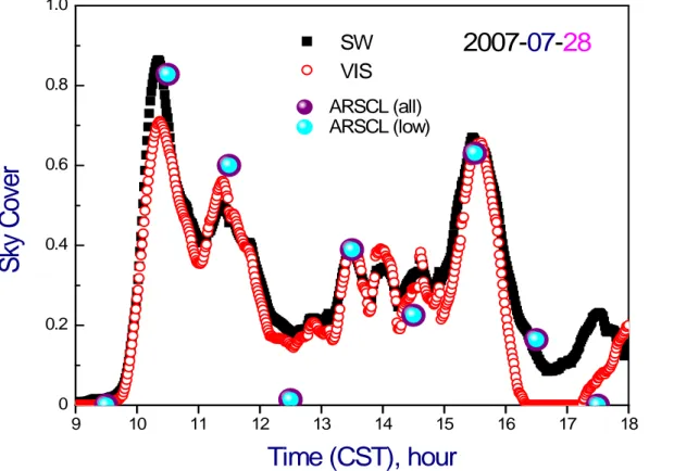
Also, we add time series of the ARSCL-based nadir-view cloud fraction. In particu-lar, 1-h averaged ARSCL cloud fraction NARSCL for low (CBH is less than 3 km) and

for all clouds are incorporated. Recall thatNSW andNvis represent hemispherical

ob-servations, while NARSCL characterizes the zenith pointing measurements. We use

the ARSCL-based properties (cloud fraction and CBH) and the TSI images to illustrate 5

how the vertical stratification of clouds and their horizontal distribution over a large area neighboring the ACRF site could contribute to the differences betweenN_SW andN_vis.

We start with comparison ofNSW andNvis for a day with low clouds only (Fig. 3). A

reasonable agreement betweenNSW andNvisis obtained for the most of the day (from

09:00 to 16:00 CST). However, a relatively large difference betweenN_SW andN_vis oc-10

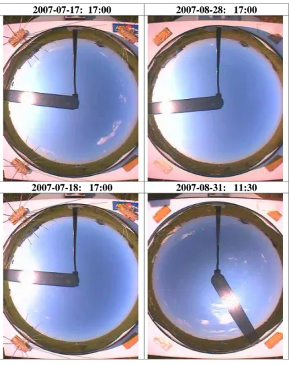
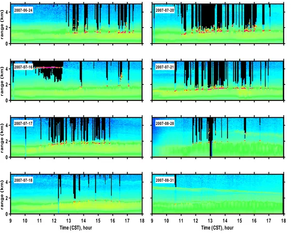
curs in the evening (from 16:00 to 18:00 CST). Are these di_fferences associated with a relative position of clouds in the sky (hemispherical FOV) and their type/abundance? Unfortunately, the TSI images are not available for this day. To address this question, we provide similar comparison for other 8 days (Fig. 4) with the accessible TSI (Fig. 5) and lidar (Fig. 6) images. For example, a similar large difference between NSW and

15

Nvisis observed in the evening (from 16 to 18) for 17 July (Fig. 4), whereNSW∼0.2 and

Nvisis zero. The corresponding TSI image includes a few optically thin clouds near the

edge (Fig. 5b). Thus, the MFRSR-based method underestimates slightly the fractional sky cover for this time period. Let us consider another example with clear-sky condi-tions observed in 28 August at 17:00 CST, whereNSW∼0.1 and Nvis is zero (Fig. 4).

20

The corresponding TSI image does not include any clouds (Fig. 5b). Therefore, the pyranometer–based method overestimates slightly the fractional sky cover for this time period. However, both the MFRSR- and pyranometer–based methods are able to pro-vide a reasonable estimation of the fractional sky cover for 31 August at 11:30 CST (Fig. 4) where a few optically thin clouds are observed (Fig. 5b).

25

For the majority of cases considered here, clouds are located below 3 km (Fig. 6). To illustrate the sensitivity of the differences betweenNSW andNvisto the vertical

(9)

AMTD

4, 715–735, 2011

E. Kassianov et al.

Title Page

Tables Figures

◭ ◮

Back Close

Full Screen / Esc

Discussion

P

a

per

|

Dis

cussion

P

a

per

|

Discussion

P

a

per

|

Discussio

n

P

a

per

the sky in the morning and noon (from 09:00 to 12:30 CST) and low cumulus clouds occur in the afternoon (Fig. 6). In general, the cumulus clouds are small (Fig. 5a). Both the MFRSR- and pyranometer–based methods capture the corresponding large diurnal changes of the fractional sky cover of middle-latitude and low clouds, and time series ofNSW and Nvis correlate reasonably well (Fig. 4). However, substantial differences

5

betweenNSW andNvis occur for some time instances (e.g., at 17:30 CST). Below, we

outline potential reasons for the observed differences.

Both Nvis and NSW represent a hemispherical measure of cloud amount, and this

measure is quite sensitive to a cloud location within hemispherical FOV. This sensitivity is more pronounced for clouds with small horizontal extent, such as cumulus clouds 10

(Kassianov et al., 2005a). For example, cloud chord length (CCL) is applied typically to characterize a representative horizontal scale of the broken clouds. We define the CCL as the length of time that an individual cloud is over a ground-based zenith-pointing instrument multiplied by the wind speed at cloud base, and found that clouds with smallest CCL (less than or equal to 0.1 km) are the most frequent (Berg and Kassianov 15

et al., 2008). Similar results are obtained for marine cumuli (e.g., Koren et al., 2008). A relatively small cloud, which partially covers the FOV, can be viewed very di_fferently by two separated instruments (Kassianov et al., 2005b). For example, the same cloud could be located in a center of MFRSR-related FOV and near to edge of pyranometer-related FOV, and vice versa. Cases with “center”- and “edge”-type cloud location are 20

characterized by large and small values of fractional sky cover, respectively (Kassianov et al., 2005a). For such instances, the MFRSR- and pyranometer-based estimations of fractional sky cover are expected to be di_fferent.

In addition to these issues associated with the instruments separation and the small-scale variability of cumulus clouds, other factors can contribute to the observed diff er-25

ences between the visibleNvisand shortwaveNSW values (Figs. 3 and 4). These

(10)

AMTD

4, 715–735, 2011

E. Kassianov et al.

Title Page

Tables Figures

◭ ◮

Back Close

Full Screen / Esc

Discussion

P

a

per

|

Dis

cussion

P

a

per

|

Discussion

P

a

per

|

Discussio

n

P

a

per

|

method (NSW) and are incorporated in the physically-based approach described here.

Despite e_ffects associated with these factors, the temporal variations ofNvis areNSW

are in a good agreement (Fig. 3 and 4). As a result, a strong linear relationship be-tween Nvis and NSW is obtained (Fig. 7a). For the majority of cases, points cluster

tightly around the slope (Fig. 7a), and the di_fference betweenNvisandNSWis less than

5

0.1 (Fig. 7b).

4 Summary

We describe a new method for estimating the fractional sky cover Nvis by using the

diffuse all-sky surface irradiances measured at two close wavelengths in the visible spectral range and their clear-sky counterparts provided by a physically-based ap-10

proach (Kassianov et al., 2010). The aerosol optical properties (aerosol optical depth, single-scattering albedo and asymmetry parameter) obtained for cloud-free time pe-riods and their temporal interpolation form the basis of this approach. To illustrate the performance of this method, we apply high-temporal resolution data from ground-based Rotating Shadowband Radiometer (MFRSR) collected during 13 days identified 15

with cumulus clouds observed in the summer of 2007 at the US Department of Energy Atmospheric Radiation Measurement (ARM) Climate Research Facility Southern Great Plains (SGP) site.

The MFRSR measures the total all-sky surface downwelling irradiance and its dif-fuse and direct components at six narrowbands centered at wavelengths of 415, 500, 20

615, 673, 870, and 940 nm (visible spectral region). ForNvis estimation, we consider

MFRSR data at two wavelengths (415 and 500 nm) only. The MFRSR observations are accompanied by shortwave measurements from a nearby broadband pyranome-ter. These shortwave measurements together with a well-established method (Long et al., 2006) give us an independent estimation of fractional sky coverNSW, which is

con-25

sidered as a reference. We compareNviswithNSW and find a strong linear relationship

(11)

AMTD

4, 715–735, 2011

E. Kassianov et al.

Title Page

Tables Figures

◭ ◮

Back Close

Full Screen / Esc

Discussion

P

a

per

|

Dis

cussion

P

a

per

|

Discussion

P

a

per

|

Discussio

n

P

a

per

Also, we demonstrate that the difference between Nvisand NSW is less than 0.1 for

the majority of cases. This favorable agreement (Nvis versusNSW) suggests that our

method based on the spectrally resolved irradiances can be applied for estimation of the fractional sky cover for different cloud types, including cumulus clouds.

The MFRSR data have been used successfully to examine changes of the water 5

vapor (Alexandrov et al., 2009), the aerosol optical and microphysical properties (Har-rison and Michalsky, 1994; Alexandrov et al., 2002; Kassianov et al., 2007; Michalsky et al., 2010), the cloud optical depth and droplet e_ffective radius (Min and Harrison, 1996), and the fractional sky cover of optically thick clouds with large horizontal size (Min et al., 2008). The method described here extends the capabilities of the MFRSR ob-10

servations by o_ffering an opportunity to sample the fractional sky cover of optically thin clouds with small horizontal size, such as shallow cumulus clouds. Thus, the worldwide deployed MFRSRs can supply an integrated dataset of the water vapor, aerosol and cloud properties, and unique MFRSR-based datasets could be developed for di_fferent locations. Such datasets together with others from ground- and satellite-based ob-15

servations can be applied to improve the understanding of the complex aerosol-cloud interactions, including the relationship between the fractional sky cover and aerosol loading and absorption.

Acknowledgements. This work has been supported by the Office of Biological and Environ-mental Research (OBER) of the US Department of Energy (DOE) as part of the Atmospheric 20

(12)

AMTD

4, 715–735, 2011

E. Kassianov et al.

Title Page

Tables Figures

◭ ◮

Back Close

Full Screen / Esc

Discussion

P

a

per

|

Dis

cussion

P

a

per

|

Discussion

P

a

per

|

Discussio

n

P

a

per

|

References

Alexandrov, M. D., Lacis, A., Carlson, B. E., and B., Cairns: Remote sensing of atmospheric aerosols and trace gases by means of Multifilter Rotating Shadowband Radiometer. Part II: climatological applications, J. Atmos. Sci., 59, 544–566, 2002.

Alexandrov, M. D., Schmid, B., Turner, D. D., Cairns, B., Oinas, V., Lacis, A. A., Gutman, 5

S. I., Westwater, E. R., Smirnov, A., and Eilers, J.: Columnar water vapor retrievals from multifilter rotating shadowband radiometer data, J. Geophys. Res., 114, D02306, doi:10.1029/2008JD010543, 2009.

Berg, L. K. and Kassianov, E. I. : Temporal variability of fair-weather cumulus statistics at the ACRF SGP site, J. Climate, 21, 3344–3358, 2008.

10

Berg, L. K., Kassianov, E. I., Long, C. N., and, Mills, D. L.: Surface summertime radiative forcing by shallow cumuli at the Atmospheric Radiation Measurement Southern Great Plains site, J. Geophys. Res., 116, D01202, doi:10.1029/2010JD014593, 2011.

Dong, X., Xi., B., and Minnis, P.: A climatology of midlatitude continental clouds from the ARM SGP Central Facility. Part II: Cloud fraction and surface radiative forcing, J. Climate, 19, 15

1765–1783, 2006.

Harrison, L. and Michalsky, J.: Objective algorithms for the retrieval of optical depths from ground-based measurements, J. Appl. Opt., 22, 5126–5132, 1994.

Kassianov, E., Long, C. N., and Ovtchinnikov, M.: Cloud sky cover versus cloud fraction: whole-sky simulations and observations, J. Appl. Meteorol., 44, 86–98, 2005a.

20

Kassianov, E., Long, C. N., and Christy, J.: Cloud-base-height estimation from paired ground-based hemispherical observations. J. Appl. Meteor., 44, 1221–1233, 2005b.

Kassianov, E. I., Flynn, C. J., Ackerman, T. P., and Barnard, J. C.: Aerosol single-scattering albedo and asymmetry parameter from MFRSR observations during the ARM Aerosol IOP 2003, Atmos. Chem. Phys., 7, 3341–3351, doi:10.5194/acp-7-3341-2007, 2007.

25

Kassianov, E., Barnard, J., Berg, L. K., Long, C. N., and Flynn, C.: Shortwave Spectral Radia-tive Forcing of Cumulus Clouds from Surface Observations, Geophys. Res. Lett., in review, 2010.

Kaufman, Y. J. and Koren, I.: Smoke and pollution aerosol effect on cloud cover, Science, 313, 655–658, 2006.

30

(13)

AMTD

4, 715–735, 2011

E. Kassianov et al.

Title Page

Tables Figures

◭ ◮

Back Close

Full Screen / Esc

Discussion

P

a

per

|

Dis

cussion

P

a

per

|

Discussion

P

a

per

|

Discussio

n

P

a

per

Long, C. N., Ackerman, T. P., Gaustad, K. L., and Cole, J. N. S.: Estimation of fractional sky cover from broadband shortwave radiometer measurements, J. Geophys. Res., 111, D11204, doi:10.1029/2005JD006475, 2006.

McComiskey, A., Schwartz, S. E., Schmid, B., Guan, H., Lewis, E. R., Ricchiazzi, P., and Ogren, J. A.: Direct aerosol forcing: Calculation from observables and sensitivities to inputs, 5

J. Geophys. Res., 113, D09202, doi:10.1029/2007JD009170, 2008.

Michalsky, J., Denn, F., Flynn, C., Hodges, G., Kiedron, P., Koontz, A., Schlemmer, J., and Schwartz, S. E.: Climatology of aerosol optical depth in north-central Oklahoma: 1992– 2008, J. Geophys. Res., 115, D07203, doi:10.1029/2009JD012197, 2010.

Min, Q. and Harrison, L. C.: Cloud properties derived from surface MFRSR measurements and 10

comparison with GOES results at the ARM SGP Site, Geophys. Res. Lett., 23, 1641–1644, doi:10.1029/96GL01488, 1996.

Min, Q., Wang, T., Long, C. N., and Duan, M.: Estimating fractional sky cover from spectral measurements, J. Geophys. Res., 113, D20208, doi:10.1029/2008JD010278, 2008.

Perlwitz, J. and Miller, R. L.: Cloud cover increase with increasing aerosol absorptivity: A coun-15

terexample to the conventional semidirect aerosol effect, J. Geophys. Res., 115, D08203, doi:10.1029/2009JD012637, 2010.

Quaas, J., Stevens, B., Stier, P., and Lohmann, U.: Interpreting the cloud cover – aerosol optical depth relationship found in satellite data using a general circulation model, Atmos. Chem. Phys., 10, 6129–6135, doi:10.5194/acp-10-6129-2010, 2010.

20

Su, W., Loeb, N. G., Xu, K. M., Schuster, G. L., and Eitzen, Z. A.: An estimate of aerosol indi-rect effect from satellite measurements with concurrent meteorological analysis, J. Geophys. Res., 115, D18219, doi:10.1029/2010JD013948, 2010.

Zhang, Y., Long, C. N., Rossow, W. B., and Dutton, E. G.: Exploiting diurnal varia-tions to evaluate the ISCCP-FD flux calculavaria-tions and radiative-flux-analysis-processed sur-25

(14)

AMTD

4, 715–735, 2011

E. Kassianov et al.

Title Page

Tables Figures

◭ ◮

Back Close

Full Screen / Esc

Discussion

P

a

per

|

Dis

cussion

P

a

per

|

Discussion

P

a

per

|

Discussio

n

P

a

per

|

10 12 14 16 18

0 0.4 0.8 0 0.5 1.0 0 0.4 0.8

c)

Time (CST), hour

R

at

io &

D

if

fer

enc

e

F*(870) / F*(415)

F(500) - F(415)

b) 415 nm

500 nm 870 nm

D

if

fus

e F

lux

O

pt

ic

al

D

ept

h

415 nm 500 nm 870 nm a)

Fig. 1. Temporal realizations of optical depth at three wavelengths (415, 500, and 870 nm)(a)

the corresponding all-sky diffuse fluxes [Wm−2_nm−1_]_{(b), and the di}

(15)

AMTD

4, 715–735, 2011

E. Kassianov et al.

Title Page

Tables Figures

◭ ◮

Back Close

Full Screen / Esc

Discussion

P

a

per

|

Dis

cussion

P

a

per

|

Discussion

P

a

per

|

Discussio

n

P

a

per

Fig. 2.Difference of diffuse fluxes at two wavelengths (415 and 500 nm) as function of time for

(16)

AMTD

4, 715–735, 2011

E. Kassianov et al.

Title Page

Tables Figures

◭ ◮

Back Close

Full Screen / Esc

Discussion

P

a

per

|

Dis

cussion

P

a

per

|

Discussion

P

a

per

|

Discussio

n

P

a

per

|

9 10 11 12 13 14 15 16 17 18 0

0.2 0.4 0.6 0.8 1.0

SW

VIS

S

ky C

o

ve

r

Time (CST), hour

2007-07-

28

ARSCL (all) ARSCL (low)

Fig. 3. Temporal realizations the visible (red) and shortwave (black) fractional sky cover for

(17)

AMTD

4, 715–735, 2011

E. Kassianov et al.

Title Page

Tables Figures

◭ ◮

Back Close

Full Screen / Esc

Discussion

P

a

per

|

Dis

cussion

P

a

per

|

Discussion

P

a

per

|

Discussio

n

P

a

per

0 0.2 0.4 0.6 0.8 1.0

9 10 11 12 13 14 15 16 17 18 0

0.2 0.4 0.6 0.8 1.0

9 10 11 12 13 14 15 16 17 18 SW

VIS

S

ky C

o

v

e

r ARSCL (all) 2007-06-24

ARSCL (low)

Sk

y C

o

ver

2007-07-16

Sk

y Co

v

e

r 2007-07-17

Sk

y Co

v

e

r

Time (CST), hour

2007-07-18

2007-07-20

2007-07-21

2007-08-28

Time (CST), hour

2007-08-31

(18)

AMTD

4, 715–735, 2011

E. Kassianov et al.

Title Page

Tables Figures

◭ ◮

Back Close

Full Screen / Esc

Discussion

P

a

per

|

Dis

cussion

P

a

per

|

Discussion

P

a

per

|

Discussio

n

P

a

per

|

2007-06-24: 17:00 2007-07-20: 16:00

2007-07-16: 17:00 2007-07-21: 17:00

Fig. 5a.Hemispherical total sky images for the first 4 days in Fig. 4. The local time (e.g., 17:00)

(19)

AMTD

4, 715–735, 2011

E. Kassianov et al.

Title Page

Tables Figures

◭ ◮

Back Close

Full Screen / Esc

Discussion

P

a

per

|

Dis

cussion

P

a

per

|

Discussion

P

a

per

|

Discussio

n

P

a

per

2007-07-17: 17:00 2007-08-28: 17:00

2007-07-18: 17:00 2007-08-31: 11:30

(20)

AMTD

4, 715–735, 2011

E. Kassianov et al.

Title Page

Tables Figures

◭ ◮

Back Close

Full Screen / Esc

Discussion

P

a

per

|

Dis

cussion

P

a

per

|

Discussion

P

a

per

|

Discussio

n

P

a

per

|

2007-06-24

r

a

n

g

e

(

k

m

)

0 2 4

2007-07-16

r

a

n

g

e

(

k

m

)

0 2 4

2007-07-17

r

a

n

g

e

(

k

m

)

0 2 4

2007-07-18

r

a

n

g

e

(

k

m

)

Time (CST), hour

9 10 11 12 13 14 15 16 17 18

0 2 4

2007-07-20

2007-07-21

2007-08-28

2007-08-31

Time (CST), hour

9 10 11 12 13 14 15 16 17 18

Fig. 6. Two-dimensional images of ground-based micropulse attenuated lidar backscatter for

(21)

AMTD

4, 715–735, 2011

E. Kassianov et al.

Title Page

Tables Figures

◭ ◮

Back Close

Full Screen / Esc

Discussion

P

a

per

|

Dis

cussion

P

a

per

|

Discussion

P

a

per

|

Discussio

n

P

a

per

0.0 0.2 0.4 0.6 0.8 1.0 0.0

0.2 0.4 0.6 0.8 1.0

N

SW

N

_vis

ρ

= 0.93

N

_SW

= 0.04 + 0.82*N

_vis

-1.0 -0.5 0.0 0.5 1.0 0 1000 2000 3000

H

is

togr

am

N

_SW

- N

_vis

Fig. 7.The visible versus shortwave fractional sky cover (left) and the corresponding difference