An Algorithm for Maximizing the Controllable Set for Open-Loop Unstable
Systems under Input Saturation
Wen-Liang, Abraham, Wang, and Yen-Ming Chen
Chung Hua University,
[email protected]
National Kaohsiung First University,
[email protected]
An optimization technique is presented for approximating the controllable set by an ellipsoid for a linear time-invariant open-loop unstable system subject to input saturation. A technique and algorithms for maximizing the controllable set are also presented. In stead of starting from a positive definite right-hand side matrix Q of the Lyapunov equation as done in almost all applications of the Lyapunov functions, we start from a positive definite Hessian matrix P for the Lyapunov function so that the resulting Lyapunov function will be convex. Keywords: input saturation, Lyapunov theorem, ellipsoidal controllable set
1.
INTRODUCTION
The concept of controllable set in control systems was introduced by Snow [1], when he defined the controllable set as the reachable set of the system with time reversed. For linear systems, there is complete duality between reachability (the ability to reach any desired final state from a given initial state) and controllability (the ability to reach a given final state from any initial state). But this is not generally true for nonlinear systems. Determination of the reachable set under input saturation has been widely studied using an open-loop approach. See Summers [2], Sabin and Summers [3], Summers, Wu and Sabin [4], and Quinn and Summers [5]. However, none of these papers covers the controllable set of a closed-loop system.
For this paper, without loss of generality, we assume that the destination state is the origin. In other
words, the controllable set is defined to be the set of the states for which there is at least one control which will drive it to the origin. For a linear time-invariant system, the controllable set is the entire state space if the system is asymptotically stable, i.e., if all the eigenvalues of the system are located on the open left-half plane. This is because the state will eventually go to the origin with zero input no matter where it starts. For an open-loop unstable linear system, i.e., a system with at least one open-loop eigenvalue on the open right-half plane or a system with at least one multiple open-loop eigenvalue on the imaginary axis, the controllable set can be made the entire state space if the open-loop system is linear stabilizable. This is because with a linear feedback control all the eigenvalues of the resulting closed-loop system can be placed on the open left-half plane thus rendering the closed-loop system asymptotically stable. However, the controllable set for the same system may not be made the entire state space, if the linear feedback is subject to input saturation.
There are two approaches for studying the controllable set of an open-loop unstable linear system:
(i) open-loop approach, in which we drive the state )
(t
x to the origin with the input u(t)restricted to ;
,..., 2 , 1 , 1 )
(t i m
ui ≤ =
(ii) closed-loop approach, in which we drive the state )
(t
x to the origin with linear feedback with saturation:
IAENG International Journal of Applied Mathematics, 36:2, IJAM_36_2_2
), ( ) ( )); ( ( ) ( t Kx t v t v sat t u = − =
where K is a constant matrix and sat(⋅) is the saturation function.
In this paper, we take the closed-loop approach and find an approximate controllable set.
2.
T
HEORYConsider a linear time-invariant continuous-time system with input saturation
) ( ) ( )
(t Axt But
x = + (1) )),
( ( )
(t sat Kxt
u =− (2) where A∈ℜn×n is a given constant matrix,
m n
B∈ℜ × is a given constant matrix, x(t)∈ℜn is the state vector, u(t)∈ℜmis the control vector, with
)], ( ),..., ( [ )
(t u1 t u t
u = m and sat(⋅) denotes the
saturation function. The one-dimensional version of the saturation function is defined by
ℜ ∈ ∀ ⎪ ⎭ ⎪ ⎬ ⎫ ⎪ ⎩ ⎪ ⎨ ⎧ − ≤ − ∈ ≥ − = y y y y y y sat , 1 ) 1 , 1 ( 1 if , 1 if , if , 1 )
( (3)
and we componentwise extend its definition to the multi-dimensional version: . , ) ( ) ( ) ( ) ( 3 2 1 m y y sat y sat y sat y
sat ∀ ∈ℜ
⎥ ⎥ ⎥ ⎥ ⎦ ⎤ ⎢ ⎢ ⎢ ⎢ ⎣ ⎡ =
# (4)
Here we assume that A is not necessarily asymptotically stable. We also assume that the system (A,B) is linearly stabilizable. In other words, it is assumed that, without saturation, the system would be stabilizable.
Hence there exists at least one matrix K such that ) ( ) ( ) ( ) ( )
(t Axt BKx t A BK xt
x = − = −
is asymptotically stable. Actually it is possible to select the location of the system eigenvalues (i.e., the eigenvalues of A-BK) arbitrarily. Hence we assume that matrix K has been selected so as to place the
system eigenvalues in the desired location. Since BK
A
A~= − is Hurwitz, for every positive definite matrix Q~ , there exists an unique
n n
P∈ℜ × satisfying
, ~ ~ ~ Q A P P
AT + =−
and P>0. Our goal is first to find an inner approximation Ω(P) of the controllable set Ω* of our system (1) and (2) based on the quadratic Lyapunov function V(ξ)=ξTPξ , and then to maximize the approximate controllable set Ω(P) by varying the approximation parameter P in such a way that the resulting matrix Q~=−(A~TP+PA~)remains positive definite.
We denote the ith row of matrix K by :
,..., 1
,i m
ki =
. 2 1 ⎥ ⎥ ⎥ ⎥ ⎦ ⎤ ⎢ ⎢ ⎢ ⎢ ⎣ ⎡ = m k k k K # .
We now consider the case of a single input. Define
) ( )
(ξ ξ sat Kξ
f =Α −Β (5)
{
}
}
{
}
{
| 1 .if , 1 | if , 1 | || if , ) ( 0 ⎪ ⎭ ⎪ ⎬ ⎫ ⎪ ⎩ ⎪ ⎨ ⎧ − ≤ ℜ ∈ = ∈ + ≥ ℜ ∈ = ∈ − < ℜ ∈ = ∈ − = + − ξ ξ ξ ξ ξ ξ ξ ξ ξ ξ ξ ξ π π π K H B A K H B A K H BK A (6)
Define )).V~(t)=V(x(t Taking derivative of )
( ~
t
V along the trajectory x(t) , we obtain the following cases:
Case 1. x(t)∈H0: unsaturated case, i.e., )
( )
(t Kxt
u =−
), ( ~ ) ( ) ( )) ( ) (( ) ( ) ( ) ( ) ( ) ( )) ( ) (( )) ( ( ) ( ) ( )) ( ( ) ( ~ t x Q t x t x BK A P P BK A t x t x BK A P t x t Px t x BK A t x Pf t x t Px t x f t V dt d T T T T T T T − = − + − = − + − = + = (7)
Case 2. x(t)∈H+:positively saturated case, i.e., 1
, ) ( ) ( ) ( ) ( ) ( ) ( ) ( ) ( ) ( ) ) ( ( ) ( ) ( ) ) ( ( )) ( ( ) ( ) ( )) ( ( ) ( ~ PB t x t Px B t Qx t x PB t x t Px B t x PA P A t x B t Ax P t x t Px B t Ax t x Pf t x t Px t x f t V dt d T T T T T T T T T T T + + − = + + + = + + + = + = (8) where ). (A P PA
Q=Δ− T + (9) Case 3. x(t)∈H−: negatively saturated case, i.e.,
1 ) (t =− u , ) ( ) ( ) ( ) ( ) ( ) ( ) ( ) ( ) ( ) ) ( ( ) ( ) ( ) ) ( ( )) ( ( ) ( ) ( )) ( ( ) ( ~ PB t x t Px B t Qx t x PB t x t Px B t x PA P A t x B t Ax P t x t Px B t Ax t x Pf t x t Px t x f t V dt d T T T T T T T T T T T − − − = − − + = − + − = + = (10)
where Q is defined as in (9).
Inspired by the right-hand sides (7), (8) and (10) for V~(t)
dt d
, we define
( )
( )
( )
, ; ; , ; , ~ 0 0 − − + + ∈ − − − = ∈ + + − = ∈ − = H PB P B Q g H PB P B Q g H Q g T T T T ξ ξ ξ ξ ξ ξ ξ ξ ξ ξ ξ ξ ξ ξ ξ ξCombining these three functions into one function, we obtain
⎪ ⎩ ⎪ ⎨ ⎧ ∈ ∈ ∈ = − − + + , if ) ( , if ) ( , if ) ( ) ( 0 0 H g H g H g g
ξ
ξ
ξ
ξ
ξ
ξ
ξ
(11)Observe that )). ( ( ) ( ~ t x g t V dt d =
We note that, in Case 1 Q~>0because P is selected so that Q~>0. In other words, because we
use only those P that will make
0 ) ~ ~ (
~=− + > A P P A
Q T , the right-hand side for
) ( ~ t V dt d
is negative: g0(ξ)≤0,∀ξ≠0. Hence }. 0 { H , 0 )
(ξ < ∀ξ∈ 0−
g Therefore, the equilibrium
point is locally asymptotically stable in H0. However, in Case 2 and 3, since the open-loop system may be unstable, matrix A may not be Hurwitz. Given a positive definite matrix P that
will make Q~>0, the Q defined by (9) may or may not be positive definite..
In order to satisfy the Lyapunov descent condition g(ξ)<0for a given ξ,we require that for each ξ≠0, there exists at least one control value νsatisfying ν ∞≤1and
. 0 2
)
(ξ =−ξ Qξ± ξ PBν <
g T T
Then the state space ℜncan be divided into the following regions:
(a) R0 =
{
ξ∈ℜn ξTQ~ξ>0}
. If ξ∈R0, then. 0 ) (ξ < g
(b) R+ =
{
ξ∈ℜn 2ξTPB<ξTQ~ξ≤0}
. If ,+ ∈R
ξ then set ν =1 so that g(ξ)<0.
(c) R− =
{
ξ∈ℜn 2ξTPB>−ξTQ~ξ≥0}
. If ,− ∈R
ξ then set ν =−1 so that g(ξ)<0.
(d) ℜn−
{
R−∪R0∪R+}
. If{
−∪ 0∪ +}
, −ℜ
∈ n R R R
ξ then it is not possible to
find ν∈[−1,1], such that g(ξ)<0.
The approach for finding the maximal level set
{
*}
*) ( )
(c V P c
LP = ξ∈ℜn ξ =ξT ξ≤ which is
contained in the union of the regions (a), (b) and (c), i.e.,
{
( )}
, max 0 * − +∪ ∪ ⊂= c L c R R R
c P
can be found by the following maximization problem
. 0 1 and , 0 ) ( subject to ) ( min * ≤ + ≥ + + − = = = + ξ ξ ξ ξ ξ ξ ξ ξ ξ K PB P B Q g P V c T T T T
see Wang, Chen, and Mukai [22].
So far we treated matrix P as a given positive definite, symmetric matrix which will make Q~>0. We now seek to find a P*which will maximize the volume (area) of the level set
{
( )}
)) (
(c* P TP c* P
and hence the volume of the approximate controllable set LP( Pc( )). We observe that, as P varies, the resulting Q~ must remain positive definite.
I. MAXIMIZE THE ELLIPSOIDAL CONTROLLABLE SET
We now introduce the procedures of finding the maximal ellipsoidal controllable set for our system (1) and (2).
Step 1
Let P=P(α,β,...)be a symmetric
n
×
n
matrix which depends on at least one parameter α, and at most2 2 ) 1 (n+ − n
parameters α ,β,.... For instance, general forms of P for n=2 and n=3 cases may be
⎥ ⎦ ⎤ ⎢ ⎣ ⎡
β α
α 1
,
⎥ ⎥ ⎥
⎦ ⎤
⎢ ⎢ ⎢
⎣ ⎡
ε δ β
δ γ α
β α 1
.
(12)
Step 2
Next, we want to maximize the level set
{
}
)
(c P c
Lp = ξ∈ℜnξT ξ≤ in which the Lyapunov criterion is satisfied. In other words, we want to maximize the value
c
subject to the constraint) (c
LP remains inside the set where the Lyapunov descent criterion g(ξ) remains negative, i.e.,
{
}
{
( ) ( ) 0}
.max ) (
* P = c L c ⊂ ξ gξ ≤
c P
Rewrite the above problem in the following way as before:
}, 1 , 0 min{
) (
* = ξ ξ −ξ ξ+ξ + ξ≥ ξ≤−
K P B PB Q
P P
c T T T T
or
}. 1 , 0 min{
) (
* P = ξ Pξ −ξ Qξ−ξ PB−B Pξ≥ Kξ≥
c T T T T
We note that the above two problems are equivalent due to symmetry.
Step 3
Finally, finding the maximal approximate controllable set (stability region) for the system is equivalent to maximizing the volume W of the maximal ellipsoid in Step 2. Therefore, the original maximization problem becomes:
. 0 and , 0 ) ~ ~ ( ~
det ) 1 2 / (
)) ( (
max
2 * 2
> >
+ − =
+ Γ =
P A
P P A Q
P n
P c W
T
n n
P
π
where W is the volume of the ellipsoid, c*(P) is the maximum level defined in Step 2, Γ(⋅) is the Gamma function, and det(P is the determinant of ) the matrix P .
Example 1
Consider the single-input open-loop unstable system
), ( ) (
), ( ) ( ) (
t Kx t u
t Bu t Ax t x
− =
+ =
where
. 1 0 , 1 2
1 0
⎥ ⎦ ⎤ ⎢ ⎣ ⎡ = ⎥ ⎦ ⎤ ⎢ ⎣ ⎡
−
= B
A
The open-loop system is unstable with eigenvalues 2
1=−
λ and λ2 =1. Suppose that the desired eigenvalues are λ~=−1+i and λ~2 =−1−i . Therefore, using a standard eigenvalue placement method, we may select a feedback matrix
[ ]
4 1 =K ,
which results in
⎥ ⎦ ⎤ ⎢
⎣ ⎡
− − = − =
2 2
1 0 ~
BK A A
whose eigenvalues are λ~1=−1+i and λ~2=−1−i as desired.
For a given positive definite matrix Q~, where .
1 0
0 1 ~
⎥ ⎦ ⎤ ⎢ ⎣ ⎡ = Q
We can find a unique symmetric, positive definite solution P, satisfying the Lyapunov equation,
⎥ ⎦ ⎤ ⎢
⎣ ⎡ =
375 . 0 25 . 0
25 . 0 25 . 1
P .
applying the method of Lee and Hedrick [14], and the controllable set under the Lyapunov descent condition [22] are shown in Figure 1 as follows.
-1 -0.5 0 0.5 1 -1
-0.8 -0.6 -0.4 -0.2 0 0.2 0.4 0.6 0.8 1
x1
x2
Fig. 1: Controllable set inside the linear unsaturated region
(inner ellipsoid) and the controllable set under Lyapunov
descent condition (outer ellipsoid)
The inner ellipsoid represents the controllable set for the system inside the linear unsaturated region, while the outer ellipsoid represents the controllable set for the system under the Lyapunov condition.
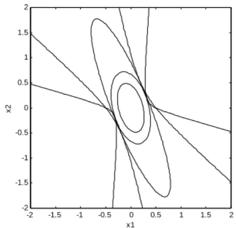
Finally, to find the maximal ellipsoidal controllable set for the system, we apply the three steps, the maximal controllable set is shown in Figure 2 as follows.
Figure 3 shows the comparison of the three controllable sets: the maximal controllable set, the controllable set under the Lyapunov descent condition, and the controllable set inside the linear region. As we can see from Fig. 3, the controllable set under the Lyapunov descent condition and the controllable set inside the linear region are contained in the maximal ellipsoidal controllable set found by our approach.
-2 -1.5 -1 -0.5 0 0.5 1 1.5 2 -2
-1.5 -1 -0.5 0 0.5 1 1.5 2
Figure 2: The maximal ellipsoidal controllable set
-2 -1.5 -1 -0.5 0 0.5 1 1.5 2 -2
-1.5 -1 -0.5 0 0.5 1 1.5 2
x1
x2
Fig. 3: Comparison of the controllable set inside the linear
region, under the Lyapunov descent condition, and the
maximal controllable set found by our approach.
Finally, we conclude this paper with a practical example, which has been studied several times in the past; see e.g., [25], [26].
Example 2 Consider the double integrator, a single input plant of the form
⎪ ⎪ ⎩ ⎪⎪ ⎨ ⎧
≤ ≤ −
⎥ ⎦ ⎤ ⎢ ⎣ ⎡ + ⎥ ⎦ ⎤ ⎢ ⎣ ⎡ =
. 1 1
, 1 0 0 0
1 0
u u x x
open-loop zero eigenvalues for the system, the system is open-loop unstable. Suppose that the desired eigenvaluesλ1′=−σ+iωand λ2′=−σ−iω for
the closed-loop system are as follows: . 1 , 2 1
1= ω = σ
For a given Q~, where
⎥ ⎦ ⎤ ⎢ ⎣ ⎡ =
1 0
0 1 ~
Q ,
the feedback gain K can be selected by the standard i pole placement technique and P can be found as follows:
[
]
.375 . 0 25 . 0
25 . 0 25 . 1 , 2
2 1
1 ⎥
⎦ ⎤ ⎢
⎣ ⎡ =
= P
K
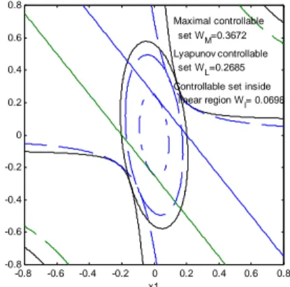
Solving the above optimization problems, we obtain the volume (area) of the ellipsoidal controllable sets as follows:
Wl=0 0698. ; WL=0 2685. ;WM =0 3672. . We denote by Wl the volume (area) found by applying the technique from Lee and Hedrick, WL the volume (area) found by applying Lyapunov descent criterion, and WM the volume (area) found by applying our technique. Figure 4 shows the volumes (areas) of the asymptotically stable region for the three techniques. Indeed, the asymptotically stable regions found by our proposed technique are superior to the other two approaches.
-0.8 -0.6 -0.4 -0.2 0 0.2 0.4 0.6 0.8 -0.8
-0.6 -0.4 -0.2 0 0.2 0.4 0.6 0.8
x1
x2
Maximal controllable set WM=0.3672 Lyapunov controllable
set WL=0.2685 Controllable set inside
linear region W
l= 0.0698
Fig. 4: Comparison of the controllable set inside the linear
region, under the Lyapunov descent condition, and the
maximal controllable set found by our approach.
3.
C
ONCLUSIONIn this paper, we presented a technique for approximating the controllable set for an open-loop unstable system under input saturation and maximized this controllable set by an ellipsoid. Instead of starting from a positive definite matrix Q as done in almost all applications of the Lyapunov functions, we reversed the approach by starting from a positive definite matrix P so that the Lyapunov function xTPx will be positive definite. Also, based on the formula for the volume of a general n-dimensional ellipsoid, we developed the algorithm of maximizing the volume of the controllable set of the system. From our example, the maximal controllable set was found and is indeed larger than those of controllable sets inside the linear region and under the Lyapunov descent condition.
A
PPENDIXWe explain why the matrix Pcan be taken in the form
⎥ ⎦ ⎤ ⎢ ⎣ ⎡
β α
α 1
, ⎥⎥
⎥
⎦ ⎤
⎢ ⎢ ⎢
⎣ ⎡
ε δ β
δ γ α
β α 1
Let Pˆbe a symmetric, positive definite matrix of the form
. ˆ ˆ
ˆ
ˆ ⎥
⎦ ⎤ ⎢ ⎣ ⎡ =
β α
α ε P
Since Pˆ is positive definite, ε >0, βˆ>0, .
0 ˆ ˆ−α2 > β
ε Note that, if we multiply both P and
. ˆ ˆ
ˆ 1 ˆ 1
⎥ ⎥ ⎥ ⎥
⎦ ⎤
⎢ ⎢ ⎢ ⎢
⎣ ⎡ =
ε β ε
α ε
α
ε P
Note that ˆ>0. ε β
Since εβˆ−αˆ2 >0,
. 0 ˆ ˆ
0 ) ˆ ˆ ( 1
2 2 2 2
> − ⇒
> −
ε α ε β
α β ε ε
Let = ˆ(>0), = ˆ(>0). ε β β ε α
α Let
. ˆ 1 1
P P
ε β α
α = ⎥ ⎦ ⎤ ⎢ ⎣ ⎡ =
The, since ˆ ˆ 0,
2 2 2 = − > −
ε α ε β α
β P is a positive
definite matrix.
R
EFERENCES[1] D. R. Snow, “Advances in Control Systems”, Edited by C. T. Leondes (New York: Academic), Vol. 5, 133-196 (1967).
[2] Nanny Summers, “Lyapunov approximation of reachable sets for uncertain linear systems”, INT. J. CONTROL, 41(5): 1235-1243 (1985).
[3] Gary C. W. Sabin and Nanny Summers, “Optimal technique for estimating the reachable set of a controlled n-dimensional linear system”, INT. J. SYSTEMS SCI., 21(4): 675-692 (1990).
[4] Danny Summers, Z. Y. Wu, and G. C. W. Sabin, “State Estimation of Linear Dynamical Systems under Bounded Control”, Journal of Optimization Theory and Applications: Vol. 72,
No. 2 (1992).
[5] J. P. Quinn and Denny Summers. “Outer ellipsoidal approximations of the reachable set at infinity for linear systems”, Journal of Optimization Theory and Applications, 89(1):
157-173 (1996).
[6] E.D. Sontag and H.J. Sussmann, “Nonlinear output feedback design for linear systems with saturating controls”, Proc. 29th IEEE Conf. Decision and Control, 3414-3416 (1990).
[7] A. R. Tell, “Global Stabilization and Restricted Tracking for Multiple Integrators with Bounded Controls”, Systems and Control Letters, 18, 165-171 (1992),.
[8] Yudi Yang, H.J. Sussmann and E.D. Sontag, “Stabilization of linear systems with bounded controls”, IFAC Nonlinear Control Systems Design, Bordeaux, France (1992).
[9] Zongli Lin and Ali Saberi, “Semi-global exponential stabilization of linear systems subject to “input saturation” via linear feedbacks”, Systems and Control Letters, No. 21, 225-239 (1993).
[10] H.J. Sussmann, E.D. Sontag and Yudi Yang, “A general result on the stabilization of linear systems using bounded controls”, IEEE Transactions on Automatic Control, Vol. 39,
NO. 12 (1994).
[11] Zongli Lin, Ali Saberi and A.R. Teel, “Simultaneous Lp-stabilization and internal stabilization of linear systems subject to input saturation-state feedback case”, Systems and Control Letters, No. 25, 219-226 (1995).
[12] R.L. Kosut, “Design of linear systems with saturating linear control and bounded states”, IEEE Transactions on Automatic Control, Vol. AC-28, No. 1 (1983).
[13] B.S. Chen and S.S. Wang, “The stability of feedback control with nonlinear saturating actuator: Time domain approach”, IEEE Transactions on Automatic control, Vol. 33, No.
5 (1988).
control saturation”, INT. J. CONTROL, 1995, Vol. 62, No. 3, pp. 619-631.
[15] M. Vidyasagar, “Nonlinear Systems Analysis” Prentice-Hall, New Jersey (1993).
[16] H.K. Khalil, “Nonlinear Systems, 2nd ed.”, Prentice-Hall, New Jersey (1996).
[17] R.C. Buck, “Advanced Calculus, 3rd ed.”, McGraw-Hill, New York (1978).
[18] Korol Borsuk, “Multidimensional Analytic Geometry”, Polish Scientific Publishers,
Warszawa, Poland (1969).
[19] P. Gill, W. Murry and M. Wright, “Practical Optimization”, Academic Press Inc. (London)
Ltd. (1981).
[20] I.S. Gradshteyn and I.M.Ryzhik, “Table of Integrals, Series and Products,” New York:
Academic Press (1965).
[21] David G. Luenberger, “Introduction to Linear and Nonlinear Programming”, Addison-Wesley
Publishing Company, 1973.
[22] Wen-Liang, Abraham, Wang, Hiro. Mukai, Yen-Ming Chen, “The Stability of State Feedback Control for Open-Loop Unstable Systems under Input Saturation”, 2003 Chinese Automatic Control Conference and
Bio-Mechatronics System Control and
Application Workshop, 307-312 (2003).
[23] Tingshu Hu, Zongli Lin, and Li Qiu, “Stabilization of Exponentially Unstable Linear Systems with Saturating Actuators”, IEEE Transactions on Automatic Control, Vol. 46, no.
6, 973-979 (2001).
[24] Ali, Saberi, Auton A. Stoorvogel, and P. Saunuti, “Control of Linear Systems with Regulation and Input Constraints”,
Springer-Verlag, (2000).
[25] Athans, M. and P.L. Falb, Optimal Control, An Introduction to the Theory and Its Applications,
McGraw-Hill, New York, U.S.A. (1966).
[26] Kirk, D.E. Optimal Control Theory—An Introduction, Englewood Cliffs, Prentice-Hall,