A Comparison of Efficient Algorithms for Scheduling Parallel Data Redistribution

Marios-Evangelos Kogias and Timotheos Aslanidis

National Technical University of Athens, Athens, Greece

A

Data redistribution in parallel is an often-addressed issue in modern computer networks. In this context, we study the case of data redistribution over a switching network. Data from the source stations need to be transferred to the destination stations in the minimum time possible. Unfortunately the time required to complete the transfer is burdened by each switching and thus producing an optimal schedule is proven to be computationally intractable. For the purposes of this paper we consider two algorithms, which have been proved to be very efficient in the past. To get improved results in comparison to previous approaches, we propose splitting the data in two clusters depending on the size of the data to be transferred. To prove the efficiency of our approach we ran experiments on all three algorithms, comparing the time span of the schedules produced as well as the running times to produce those schedules. The test cases we ran indicate that not only our newly proposed algorithm yields better results in terms of the schedule produced but runs faster as well.

K

parallel, distributed, package, scheduling, setup cost, approximation, preemption

1.

I

As the need for communication and dissemination of information increases in modern technology based societies, so does the need for faster and more efficient networks and routing of packages between stations. In this context the study of parallel machines (parallel supercomputers, symmetric multiprocessors, multicomputer clusters and IP router switch fabrics), communication backbones interconnecting the machines and the transfer of large packets of data between them, has become an issue of major importance. As information loads continue to increase rapidly, it is expected that the need for well scheduled data transfers that decrease time and resource usage, will keep on being an often addressed subject for many computer scientists and engineers.

any interruption of packages transfer will come with a time cost. Information on the data remains that were not transferred along with the main part of the package, have to be saved and a new setup has to be initiated for the next package to start transferring. Consequently prior to sending any of the packages there will be a setup overhead. We consider this overhead to be constant for all transfer initiations. In this paper we aim to minimize the duration of the aforementioned process.

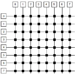
Figure 1. Crossbar switch interconnection network

2.

P

R

PBS has been proven to be NP-Hard in [8], and 4/3- inapproximable for any >0, unless P=NP in [4].

As PBS algorithms can be implemented in various applications, many polynomial time algorithms have been designed to produce solutions close to the optimal, found in [1], [4], [5],

[6]. The optimal approximation ratio proven so far is 2 1 d 1

−

+ , where d is the setup cost. Proof of

that can be found in [1]. Tests on the performance of numerous algorithms producing near-optimal solutions are presented in [4], [5], [6] and [10].

The optimal solution can be found in polynomial time if the setup cost is zero and in the case we are only interested in minimizing the number of preemptions [8]. Finally, in [1] can be found a polynomial time algorithm to calculate the optimal solution for a class of graphs that the authors define.

The performance of our algorithm is compared to that of 2 algorithms found in bibliography:

• _{A-PBS(d+1), which has the best approximation ratio proven so far [1].} • A1, which appears to perform very well in practice [6].

To schedule each data package, A-PBS(d+1) rounds up the time of each transfer to the closest multiple of d+1 and calculates the package reducing the workload of each station to the minimum multiple of d+1.

3.

G

Our data representation will be through a bipartite graph G(V,U,E). V will be the set of source stations, U the set of receiving stations while E, the set of edges, will correspond to the data loads that have to be transferred from V to U. A weight (or cost) c(v,u), will be assigned to each of the edges e=(v,u), to denote the time required to transfer the data from node v to node u. Edge weights are considered to be non-negative integers.

Furthermore the following notation will be used: = (G)=max{ v V

max(deg(v))

∈ ,max(deg(u))u U∈ }, that is, will denote the maximum number of data transfers from or to any of the stations. The function t: V∪U→Z+ will denote the total workload of any station, namely t(v)=

u U c(v, u) ∈ for any v∈V or t(u)=

v V c(v, u) ∈

for any u∈U.

W=W(G)=max{ v V max(t(v))

∈ ,max(t(u))u U∈ }, that is W will denote the maximum total transfer time

from or to any station. d∈_Z*

+ will denote the overhead to start the next transfer.

The objective function to be minimized is C(G,d)= S

i i 1

T(p ) =

+d S, where S is the number of data

packages and T(pi) is the time required for each package pi, to be transferred.

A lower bound to the optimal solution is W(G)+d (G). Yet, this lower bound is not always achievable as shown in [6].

4.

T

S

G

A

For the purposes of our algorithm the initial graph is split in two parts. GM comprises edges of weight at least d and Gm contains all edges of weight less than d. Our main concern for GM is to keep reducing the workload for each of the stations, achieving the minimum transfer time possible, whereas in the case of Gm, where edge weights are small in comparison to d, we aim in minimizing the number of preemptions. The intuition in designing this algorithm is that for data transfers of long duration, priority on how to schedule has the duration of the data transfer rather than the number of preemptions, whilst for data transfers of shortest duration prioritized is the minimization of the number of preemptions. In particular:

The Split-Graph Algorithm (SGA)

Step 1: Split the initial graph G(V,U,E) in two bipartite graphs Gm(Vm,Um,Em) and GM(VM,UM,EM), where Vm=VM=V, Um=UM=U and Em contains all edges of weight less than d, EM contains all edges of weight d or more. Clearly in this initiation step E=Em∪EM and Em∩EM=∅.

Step 2: Use subroutine1 to find a maximal matching M, in GM.

Step 3: Use subroutine 2 to calculate the weight of the matching to be removed. Remove the corresponding parts of the edges.

Step 4: If possible, add edges to M, from Em to maximize |M| and remove them from Em. Step 5: Move edges of weight less than d, from the graph induced by step 3 to Em. Step 6: Repeat steps 2 to 5 until all edges initially in EM have been completely removed.

Step 8: Schedule the data packets as calculated in steps 2, 3 and 7.

Subroutine 1:

Step 1: M=∅ _{(Initialization of the matching).}

Step 2: For each node w∈_VM∪_{UM calculate t(w).}

Step 3: Sort all nodes w∈_VM∪_{UM in decreasing order of t(w). Let L be the induced list of nodes.}

Step 4: Let w0 be the 1st node to appear in L. Run sequential search in L to find the 1st neighbour of w0 appearing in L. Denote that neighbour by w1.

Step 5: M←M∪{w0, w1}. Step 6: Remove w0, w1 from L.

Step 7: Repeat steps 2, to 6 until M becomes maximal.

Subroutine 2:

Step 1: For each edge e=(v,u) of the matching M, with corresponding weight c(e) calculate what the value W(Ge) of the induced graph Ge(Ve,Ue,Ee) would be if all edge weights in the matching were to be reduced by c(e). In this case edges in M, of cost less than c(e) would be completely removed.

Step2: For all e∈_{M, set r(e)=c(e)+W(Ge) and denote by e0 the edge such that}

r(e0)=min{r(e)|e∈M} and c(e0)=max{c(e)|r(e)=r(e0)}.

Step 3: For each edge e, in M set its new weight c(e)= c(e) c(e ), if c(e)0 c(e )0 0, otherwise

− >

.

Subroutine 3:

Step 1: Add nodes and edges to make Gm a regular graph of degree m. New edges will be of zero weight. In a regular graph, all nodes will be of the same degree.

Step 2: Calculate a maximum matching Mm in Gm and remove all edges of Mm from Gm. Gm’s degree will now be reduced by 1.

Step 3: Repeat step 2 until Gm=∅. Example:

Consider matrix A to be the adjacency matrix of G(V, U, E), where V={a1, b1, c1, d1}, U={a2, b2, c2}. Rows 1, 2, 3 and 4, show the times required to transfer the data from nodes a1, b1, c1, d1 respectively, while columns 1, 2 and 3 stand for the durations needed to transfer the data to a2, b2, c2, respectively. Suppose d=3.

5 3 2 1 4 3 A

2 5 0 4 2 5

=

Let AM be the adjacency matrix corresponding to GM and Am be the adjacency matrix of Gm. Then:

M

5 3 0

0 4 3 A

0 5 0 4 0 5

= m

0 0 2

1 0 0 A

2 0 0 0 2 0

t(a1)=8, t(b1)=7, t(c1)=5, t(d1)=9, t(a2)=9, t(b2)=12, t(c2)=8. sorting the nodes: b2, d1, a2, a1, c2, b1, c1.

M={{b2,a1}, {d1,c2}}, e0={d1,c2}, r(e0)=14.

Add edge {b1,a2}∈Em to M. Schedule a transfer of duration 5 Total time for this iteration including preemption cost is 8 The induced matrices after the 1st iteration are:

M

5 0 0

0 4 3 A

0 5 0 4 0 0

= _,

m

0 0 2

0 0 0 A

2 0 0 0 2 0

=

t(a1)=5, t(b1)=7, t(c1)=5, t(d1)=4, t(a2)=9, t(b2)=9, t(c2)=3 sorting the nodes: a2, b2, b1, a1, c1, d1, c2

M={{a2,a1},{b2,b1}} e0={a2,a1}, r(e0)=10.

No additional edge from Em. Schedule a transfer of duration 5 Total time for this iteration including preemption cost is 8 The induced matrices after the 2nd iteration are:

M

0 0 0 0 0 3 A

0 5 0 4 0 0

= _,

m

0 0 2 0 0 0 A

2 0 0 0 2 0

=

t(a1)=0, t(b1)=3, t(c1)=5, t(d1)=4, t(a2)=4, t(b2)=5, t(c2)=3 sorting the nodes: c1, b2, d1, a2, b1, c2, a1.

M={{c1,b2},{d1,a2},{b1,c2}} e0={c1,b2}, r(e0)=5.

No additional edge from Em. Schedule a transfer of duration 5 Total time for this iteration including preemption cost is 8. All edges in EM are now removed, proceeding to step 7 of SGA:

m

0 0 2

0 0 0 A

2 0 0 0 2 0

=

The corresponding maximum matching is M={{a1,c2}, {c1,a2}, {d1,b2}} The duration of the scheduled transfer is 2.

Total time for this iteration including preemption cost is 5.

Total time to transfer the data is 29, while the lower bound is 26.

5.

C

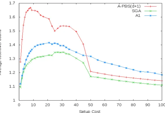
S

better than both A1 and A-PBS(d+1) and as the overhead increases it shows an increasingly improved performance. It is important to mention that in practice, as information loads exponentially increase, the number of stations and communication tasks increases and so does the setup cost. That is in fact the most encountered situation nowadays.

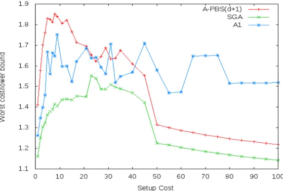
Figure 3 presents the worst performance that each algorithm had depending on the setup cost, in terms of proximity to the lower bound again. SGA is found to be once again a lot more efficient. Furthermore, SGA in most cases has a worst case really close to the average showing that its performance does not fluctuate much, making it an all cases reliable tool for this type of scheduling.

It is important to stress out that the ratio calculated, is in comparison to the lower bound and not to the optimal value of the objective function. Therefore the schedules produced are in fact a lot closer to the optimal and the ratios a lot closer to 1.

Figure 3. Worst (cost/lower bound) comparison

6.

C

R

T

To compare time complexities for the 3 algorithms we will assume that |E|=m and we will denote max{|V|,|U|}=n.

All three algorithms compared, will need O(m) iterations to produce a schedule as it is certain that each iteration will result in the complete removal of at least one edge.

For each iteration the most time consuming subroutine of A-PBS(d+1) is finding a maximum matching which will need O( n m) [12]. Therefore the overall complexity of A-PBS(d+1) is O( n m2)

As far as A1 is concerned, determining how to preempt is the most time consuming subroutine for each iteration. For each of the edge weights in the matching, it calculates for each node v, deg(v) and t(v). Each of these three processes requires O(n), therefore the complexity of each iteration is O(n3) making the overall time complexity O(n3m).

Finally, the complexity of SGA is determined by the maximum matching process that takes place in step2 of subroutine3 and consequently the overall complexity is the same as that of A-PBS(d+1), namely O( n m2).

7.

C

F

W

Our newly presented algorithm (SGA), has proven to produce more efficient schedules. We believe that the idea of splitting the initial graph in parts can be further researched and depending on the magnitude of the edges as well as the setup cost, the Split-Graph Algorithm’s efficiency can be further improved. An approximation ratio for SGA could be established to be less than 2. Exploiting to a greater extend algorithms that provide optimal solutions for special instances of the problem might also yield interesting new approximation algorithms. Finally, lifting limitations of the problem or introducing new ones could help in identifying new classes of graphs for which polynomial algorithms might provide an optimal schedule.

R

[1] F. Afrati, T. Aslanidis, E. Bampis, I. Milis, Scheduling in Switching Networks with Set-up Delays. Journal of Combinatorial Optimization, vol. 9, issue 1, p.49-57, Feb 2005.

[2] P. B. Bhat, V. K. Prasanna and C. S. Raghavendra, Block Cyclic Redistribution over Heterogeneous Networks, in 11th International Conference on Parallel and Distributed Computing Systems (PDCS 1998), 1998.

[3] G. Bongiovanni, D. Coppersmith and C. K.Wong, An optimal time slot assignment for an SS/TDMA system with variable number of transponders, IEEE Trans. Commun. vol. 29, p. 721-726, 1981.

[4] J. Cohen, E. Jeannot, N. Padoy and F. Wagner, Messages Scheduling for Parallel Data Redistribution between Clusters, IEEE Transactions on Parallel and Distributed Systems, vol. 17, Number 10, p. 1163, 2006.

[5] J. Cohen, E. Jeannot, N. Padoy, Parallel Data Redistribution Over a Backbone, Technical Report RR-4725, INRIA-Lorraine, February 2003.

[6] P. Crescenzi, X. Deng, C. H. Papadimitriou, On approximating a scheduling problem, Journal of Combinatorial Optimization, vol. 5, p. 287-297, 2001.

[7] I. S. Gopal, G. Bongiovanni, M. A. Bonucelli, D. T. Tang, C. K. Wong, An optimal switching algorithm for multibeam satellite systems with variable bandwidth beams, IEEE Trans. Commun. vol. 30, p. 2475-2481, Nov. 1982.

[8] I. S. Gopal, C. K. Wong, Minimizing the number of switchings in an SS/TDMA system IEEE Trans. Commun. vol. 33, p. 497-501, 1985.

[9] T. Inukai, An efficient SS/TDMA time slot assignment algorithm IEEE Trans. Commun. vol 27, p. 1449-1455, Oct. 1979.

[10] E. Jeannot and F. Wagner, Two fast and efficient message scheduling algorithms for data redistribution over a backbone, 18th International Parallel and Distributed Processing Symposium, 2004.

[11] A. Kesselman and K. Kogan, Nonpreemptive Scheduling of Optical Switches, IEEE Transactions in Communications, vol. 55, number 6, p. 1212, 2007.

[12] S. Micali and V. V. Vazirani, An O( | V | |E|) algorithm for finding a maximum matching in general graphs, in Proc. 21st Ann IEEE Symp. Foundations of Computer Science, p. 17-27, 1980.

[13] K. S. Natarajan and S. B. Calo, Time slot assignment in an SS/TDMA system with minimum switchings IBM Res. Rep. 1981.

Authors

Timotheos Aslanidis was born in Athens, Greece in 1974. He received his Mathematics degree from the University of Athens in 1997 and a master's degree in computer science in 2001. He is currently a phd candidate at the National and Technical University of Athens in the department of electrical and computer engineering. His research interests comprise but are not limited to computer theory, number theory, network algorithms and data mining algorithms.