F
A Pattern Langu
Pedr
Universidade Nova de Lisboa
Faculdade de Ciências e Tecnologia
Departamento de Informática
guage for Parallelizing Irregular
dro Miguel Ferreira Costa Monteiro
Dissertação apresentada na Faculdad Tecnologia da Universidade Nova Obtenção do grau de Mestre em Engenh
Orientador: Prof. Doutor Miguel Pessoa
Lisboa
2010
lar Algorithms
iro
ade de Ciências e a de Lisboa para nharia Informática
3
Acknowledgements
The challenges proposed by a MSc dissertation are many and require not only hard work, but also constant support, care and attention. To those who have accompanied me, I leave my thanks:
None of this would have been possible without the unconditional support and encouragement of my family and friends. My mother and sister, who never lost faith in me in all this years. My nephews, whose thoughts gave me strength. My better half, who gave me a purpose. All my close friends, who have accompanied me in this long road, especially João and Tiago, the former for motivating me in the beginning of this journey and the latter for being with me until the end. Many thanks also to Nuno, my closest friend and without whose constant concern and motivation most of this would not have been accomplished. I must also thank all colleagues of the Centre for Documentation and Library, many of which I am proud to call my friends: Filomena, Salima, Lina, Rosário, Ana. All who have encouraged me and helped me reach this stage.
Special thanks are also merited by Professor Miguel Monteiro, my MSc supervisor, for his inspiration, support, and constructive criticism which always pushed me to do better.
4
5
Resumo
Em algoritmos irregulares, as dependências e distribuições dos conjuntos de dados não podem ser previstas de forma estática.
Esta classe de algoritmos tende a organizar as computações consoante a localização dos dados em vez de paralelizar o controlo em múltiplas threads. Assim, as oportunidades para explorar paralelismo variam dinamicamente conforme o algoritmo altera a dependência entre os dados. O que leva a que a paralelização eficaz desses algoritmos exija novas abordagens que tenham em conta essa natureza dinâmica.
Esta dissertação procura resolver o problema da criação de implementações paralelas eficientes através de uma abordagem que propõe a extracção, análise e documentação de padrões de concorrência e paralelismo presentes na framework Galois para paralelismo de algoritmos irregulares. Padrões são representações formais de uma possível solução de um problema que surge num contexto bem definido de um domínio específico.
Os padrões referidos são documentados através de uma linguagem de padrões que evidência um conjunto de padrões inter-dependentes, que compõe um modelo de uma solução que pode ser reutilizada sempre que um problema especifico surja.
Palavras-Chave:
Linguagem de Padrões Algoritmos Irregulares Computação Paralela Engenharia Reversa
6
7
Abstract
In irregular algorithms, data set’s dependences and distributions cannot be statically predicted. This class of algorithms tends to organize computations in terms of data locality instead of parallelizing control in multiple threads. Thus, opportunities for exploiting parallelism vary dynamically, according to how the algorithm changes data dependences. As such, effective parallelization of such algorithms requires new approaches that account for that dynamic nature.
This dissertation addresses the problem of building efficient parallel implementations of irregular algorithms by proposing to extract, analyze and document patterns of concurrency and parallelism present in the Galois parallelization framework for irregular algorithms. Patterns capture formal representations of a tangible solution to a problem that arises in a well defined context within a specific domain.
We document the said patterns in a pattern language, i.e., a set of inter-dependent patterns that compose well-documented template solutions that can be reused whenever a certain problem arises in a well-known context.
Keywords:
Pattern language Irregular Algorithms Parallel Computing Reverse Engineering
8
9
Table of Contents
1
1 INTRODUCTION ... 15
1.1 MOTIVATION ... 15
1.2 CONTRIBUTIONS ... 16
1.3 STRUCTURE ... 16
2 2 IRREGULAR ALGORITHMS ... 19
2.1 AMORPHOUS DATA PARALLELISM ... 20
2.2 CATEGORIZATION OF IRREGULAR ALGORITHMS ... 20
3 3 THE GALOIS FRAMEWORK ... 23
3.1 GALOIS EXECUTION MODEL ... 24
3.2 WORKLIST-BASED ALGORITHMS ... 25
3.3 GALOIS TERMINOLOGY ... 26
4 4 IRREGULAR ALGORITHMS IN GALOIS ... 27
4.1 DELAUNAY TRIANGULATION ALGORITHM ... 28
4.2 PREFLOW-PUSH ALGORITHM ... 31
4.3 SPARSE CHOLESKY FACTORIZATION ALGORITHM ... 34
4.4 KRUSKAL’S MINIMUM SPANNING TREE ALGORITHM ... 36
5 5 ARCLIGHT PLUGIN ... 39
6 6 PATTERNS AND PATTERN LANGUAGES ... 43
6.1 PATTERNS ... 43
6.2 PATTERN LANGUAGES ... 45
6.3 FORM AND STYLE ... 46
7 7 PATTERN LANGUAGE ... 49
7.1 PATTERN TERMINOLOGY ... 52
7.2 ALGORITHM STRUCTURE PATTERNS ... 53
7.2.1 Amorphous Data-Parallelism ... 53
7.2.2 Optimistic Iteration ... 59
10
7.3 ALGORITHM EXECUTION PATTERNS ...77
7.3.1 In-order Iteration ...77
7.3.2 Graph partitioning ...82
7.3.3 Graph Partition Execution Strategy ...89
7.4 ALGORITHM OPTIMIZATION PATTERNS ...95
7.4.1 One-Shot ...95
7.4.2 Iteration Chunking ... 100
7.4.3 Preemptive Read ... 105
7.4.4 Lock Reallocation ... 109
8 8 RELATED WORK ... 113
9 9 CONCLUSIONS AND FUTURE WORK ... 117
9.1 FUTURE WORK ... 118
11
List of Figures
FIG.1–CATEGORICAL DIVISION OF IRREGULAR GRAPH ALGORITHMS. ... 20
FIG.2–DIFFERENT GRAPH TOPOLOGIES IN IRREGULAR ALGORITHMS ... 21
FIG.3-ACTION OF THE DIFFERENT COMPUTATIONAL OPERATORS ... 22
FIG.4–GALOIS OPTIMISTIC EXECUTION MODEL. ... 24
FIG.5–FOREACH SET ITERATOR IN GALOIS. ... 24
FIG.6–GALOIS ABSTRACTIONS FOR IRREGULAR ALGORITHMS ... 26
FIG.7–EXAMPLE EXECUTION OF THE DELAUNAY TRIANGULATION ALGORITHM ... 29
FIG.8–CLASSIFICATION OF THE DELAUNAY TRIANGULATION ALGORITHM. ... 30
FIG.9–EXAMPLE EXECUTION OF THE PREFLOW-PUSH ALGORITHM ... 32
FIG.10–CLASSIFICATION OF THE PREFLOW-PUSH ALGORITHM. ... 33
FIG.11–CLASSIFICATION OF THE SPARSE CHOLESKY FACTORIZATION ALGORITHM. ... 36
FIG.12–CLASSIFICATION OF KRUSKAL’S MST ALGORITHM. ... 37
FIG.13–ARCHLIGHT PLUGIN TOOLBAR. ... 40
FIG.14–ARCHLIGHT ECLIPSE PLUGIN CONCERN COLORING. ... 40
FIG.16–PERCENTAGE OF GALOIS CODE IN THE CODE OF IRREGULAR ALGORITHMS ... 41
FIG.15–ARCHLIGHT ECLIPSE PLUGIN. ... 41
FIG.17–OVERVIEW OF THE PATTERN CATALOGUE. ... 49
FIG.18–EXPLICIT RELATIONSHIPS AMONG PATTERNS. ... 51
FIG.19–HIERARCHICAL INTERFACE MODEL OF GALOIS’DATA-STRUCTURES. ... 74
FIG.20–GRAPH REPRESENTATIONS OF A SPARSE SYMMETRICAL MATRIX. ... 75
FIG.21–GRAPH PARTITIONING ... 85
FIG.22–PARTITIONED PREFLOW-PUSH GRAPH ... 87
FIG.23–REDUNDANT COPY OF BORDERING NODES ... 91
12
13
Code Listings
LISTING 1–ITERATIVE WORKLIST ALGORITHM. ... 26
LISTING 2–WORKLIST ALGORITHM IN GALOIS. ... 28
LISTING 3–DELAUNEY TRIANGULATION ALGORITHM IN GALOIS. ... 30
LISTING 4–PREFLOWPUSH ALGORITHM IN GALOIS. ... 33
LISTING 5–SPARSE COLUMN-CHOLESKY FACTORIZATION ALGORITHM. ... 34
LISTING 6–GALOIS’GRAPH-BASED CHOLESKY FACTORIZATION ALGORITHM. ... 35
LISTING 7–GALOIS IMPLEMENTATION OF KRUSKAL’S MST ... 37
LISTING 8–SEQUENTIAL DELAUNEY TRIANGULATION ... 57
LISTING 9–GALOIS’PARALLEL DELAUNEY TRIANGULATION ... 57
LISTING 10–COMMUTATIVITY AND INVERSE OF A GALOIS LIBRARY METHOD. ... 65
LISTING 11–OPTIMISTIC IMPLEMENTATION OF DELAUNEY TRIANGULATION. ... 66
LISTING 12–MATRIX TO GRAPH TRANSFORMATION. ... 76
LISTING 13–ORDERED IN GALOIS’ FOREACH ITERATOR. ... 80
LISTING 14–IN-ORDER IMPLEMENTATION OF KRUSKAL’S MST. ... 81
LISTING 15–GRAPH PARTITIONING IN GALOIS. ... 86
LISTING 16–GALOIS PARTITION EXECUTION STRATEGY. ... 94
LISTING 17–ONE-SHOT PATTERN IN GALOIS. ... 98
LISTING 18–CHUNKING OF ITERATIONS WITH GLOBAL WORKLIST. ... 102
LISTING 19–CHUNKING OF ITERATIONS WITH THREAD-LOCAL WORKLIST. ... 103
14
15
1
1
Introduction
This dissertation presents and documents a pattern language for parallelizing irregular algorithms. The body of work produced in this dissertation builds upon the work produced at the University of Texas in Austin, namely the Galois framework, and was partly supported by the project Parallel Refinements for Irregular Applications(UTAustin/CA/0056/2008) funded by FCT-MCTES and European funds (FEDER).
1.1 Motivation
Gustafson’s law [1] states that any sufficiently large problem can be efficiently parallelized and has proven that parallelization is an effective way to accelerate the processing of massive data. However, in practice not all applications are easily parallelized and finding the right programming model and architecture for a given algorithm is quite challenging in the multicore era. Issues such as race conditions, communication, scalability, load balancing, data distribution, and locality further add to the effort of achieving efficient parallel programs.
Many approaches, methodologies, libraries, languages and frameworks have been devised and these are, for the majority of algorithms, able to produce efficient parallel implementations. Aside from those “regular” algorithms, not much attention has been granted to the so-called irregular algorithms and applications [2]. The parallelization of irregular algorithms [3-4] is constrained by irregular accesses to dynamic pointer-based data structures whose data-dependence set can only be uncovered at run-time. In this context irregular algorithms pose a challenging problem to current parallelization methods and techniques.
16
Patterns capture formal solutions to specific problems, while maintaining a level of abstraction similar to that of design models (e.g., UML) and above source code. This way, patterns support a high-level form of reuse, which is independent from language, paradigm and hardware. Identifying and documenting patterns of complex concurrent software problems is one of key practices that will allow concurrent software development to be established as an engineering discipline – one which requires thorough systematic understanding and documentation of successful practices [5].
Pattern catalogs and languages for software design represent a widely prolific area of development, partly due to the renowned Gang of Four catalog of object-oriented design patterns [6]. From this first approach, patterns became popular in the field of reusable design, branching different application areas such as object-oriented programming [7], aspect-oriented programming [8] framework design [9-10], software architecture [11-12], components [13], machine learning [14-15] and even patterns about patterns [16-17].
1.2 Contributions
To the best of our knowledge, this pattern language is the first to address specific solutions to the problems of irregular algorithms. We have described a set of ten patterns for parallelizing irregular algorithms. These present knowledge derived from the Galois framework, which was in turn inherited from years of insights and experiences on parallel software development. Additionally they present a high-level approach that allows for the dissemination of knowledge that before was property of expert parallel software developers. Furthermore, the set of patterns is documented as a Pattern Language, i.e. set of inter-dependent patterns. Pattern languages guide pattern-oriented software development, such that choosing to use one pattern will eventually direct the software developer to use another related pattern. Following the sequence of pattern dependences will eventually lead to an efficient parallelization of an irregular algorithm.
1.3 Structure
The remainder of this dissertation is organized as follows:
- Chapter 2 overviews the problem being tackled by providing an overview of the
17
Finally, some insight is given as to how these algorithms can be categorized in order to provide reusable abstractions (section 2.2).
- Chapter 3 presents the Galois framework and provides a general overview of the
Galois Execution Model (section 0). It follows by describing worklist-based implementation of irregular algorithms in Galois (section 3.2 ). This chapter concludes by presenting some Galois specific terminology in section 3.3 .
- Chapter 4 describes some irregular algorithms and provides the appropriate
implementations in the Galois framework. The set of irregular algorithms is comprised of: Delaunay Triangulation, an algorithm for the generation of triangular meshes (aection 4.1), Preflow-Push, a max-flow algorithm (section 4.2), Sparse Cholesky Factorization, a traditional linear algebra algorithm for matrix factorization (section 4.3) and Kruskal’s Minimum Spanning Tree (section 4.4).
- Chapter 5 describes the Archlight Eclipse plugin, which was implemented to extract
metrics from Galois and determine the viability of our pattern mining approach.
- Chapter 6 describes the concept of pattern (section 6.1), pattern languages (section
6.2) and introduces the general form as style of patterns description (section 6.2).
- Chapter 7 presents the pattern language and contextualizes it by proposing some
abstract terminology used in the pattern descriptions (section 7.1). The next three sections document the set of patterns that compose our pattern language: Structure Patterns in section 7.2, Execution Patterns in section 7.3 and Optimization Patterns
in section 7.4. Each section is further refined into the specific patterns.
- Chapter 8 presents an overview of related work in the field of pattern languages for
parallel computing.
- Chapter 9 describes a summary of contributions and a discussion of future work.
18
19
2
2
Irregular Algorithms
The programming community is not always in harmony and although algorithm irregularity is frequently considered in the literature, there is no consensual definition of what in fact constitutes an irregular algorithm. Some authors refer to irregular algorithms as those on whichdata is structured as multidimensional arrays and referenced through array indirections and indexed values [18-19]. Other authors consider that the irregularity factor is due to the dynamism of pointer-based data-structures [20-22]. There are others even that consider algorithms to be irregular due to input dependent communication patterns [23] or irregular data distribution among the processors [24].
Our view is that, although there is no consensus on a single definition, in fact there is a clear pattern among different descriptions. Most references to irregularity as a problem of indirect access to data can be found in articles published until around the mid 1990s, roughly when object-oriented programming became widespread in the programming community [25]. From hereafter, object-orientation, and essentially pointer-based programming, became the tool of choice for the implementation of most algorithms, including irregular, giving rise to the second definition. The following two definitions arise from the fact that, in pointer-based data-structures, growth can be unpredictable, which will easily lead to irregular distributions of data among partitions and of tasks required to handle such data.
20 2.1 Amorphous data parallelism
Irregular algorithms are data-parallel algorithms [27] and essentially perform multiple operations on large data-sets, organizing computations in terms of data locality instead of parallelizing control in multiple threads. When data-set’s dependencies and distributions are unpredictable and dynamic, as in the case of implementations of irregular algorithms, the amount of parallelism that can be achieved varies according to how the algorithm changes its data dependences. As such, effective parallelization of irregular algorithms requires new approaches that account for the dynamic nature this class of algorithms.
Amorphous data-parallelism [20], is the type of parallelism that arises when the data-sets being iterated have no fixed shape or size, i.e. are amorphous. This means that the amount of available opportunities for concurrency-free parallelism changes throughout the execution of the algorithm. It is an example of data-parallelism in which simultaneous operations may interfere with each other and in which the underlying data-structure might be modified.
2.2 Categorization of irregular algorithms
Pingali et al [20] present a general categorical division of irregular algorithms that allows the reuse of patterns of parallelism and locality common to these algorithms. This categorization, shown in Fig. 1, provides a simple yet expressive way to address the implementation of irregular algorithms.
A detail description of each category is described next:
The topology category pertains to the overall shape of the data-structure. The general form is that of a simple graph (Fig. 2-a). The two other types of graphs are special forms of sparse graphs, which have relatively few edges. Trees are special graphs where there are no cycles
Irregular Graph Algorithms
Topology Operator Ordering
Graph Grid Tree Morph Local Computation Reader unordered ordered
21
and the starting node is called root (Fig. 2-b). A grid is a graph in which every node is connected to four neighbors (Fig. 2-c).
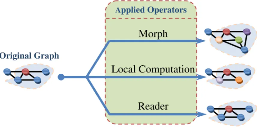
The computational operator is classified in terms of how the active node neighborhood is changed by the action of the operator (Fig. 3). The operator of an algorithm can be one of three types: Morph, Local Computation and Reader.
Morph algorithms
Morph algorithms considerably change the structure of the graph by adding or removing nodes and edges. This can be done by either coarsening, refinement or
reduction. Coarsening algorithms iteratively collapse adjacent nodes together until the graph forms a coarser sub-graph. Boruvka’s MST algorithm, for example, builds the minimum spanning tree bottom-up by coarsening [28]. Contrary to coarsening,
refinement algorithms iteratively generate the output graph from a subset of the nodes. This is the case of Delaunay Triangulation [4, 29] and Delaunay Mesh Refinement
[30]. Reduction algorithms are similar to coarsening but simply remove nodes and edges from the graph, not actually contracting elements [31-32].
Local Computation Algorithms
This class of algorithm operator does not modify the underlying graph structure but instead updates its labels and data elements (e.g. Preflow-push algorithm [33] ).
Reader Algorithms
This type of operator only reads the graph and does not modify it in any way.
The type of operator is inferred to be the type with most computational impact, i.e., if an irregular algorithm performs a read and a morph, the type of operator present in the algorithm is considered to be a morph operator.
Fig. 2 – Different graph topologies in irregular algorithms
22
The ordering of execution of an iteration must be chosen so as to avoid data-races and consistency problems. Unordered execution is the case where the sequence in which nodes are executed has a non-deterministic aspect, meaning that output is independent of this same sequence. Ordered execution implies that the output of the algorithm is influenced by the sequence by which nodes are executed. The order might be full or only partial but nevertheless parallelization of execution on ordered sets is difficult to implement, because it requires a more restricting scheduling policy. A sense of ordering can be represented by directional graphs.
Fig. 3 - Action of the different Computational Operators Applied Operators
Morph
Local Computation
Reader
23
3
3
The Galois Framework
This chapter presents the Galois framework [2, 34] which tackles the problems that arise from trying to parallelize irregular algorithms and applications (chapter 2). It does so by building upon the categorization presented in section 2.1 .
As stated in chapter 2, irregular algorithms are often associated with the scientific community. The effort needed to create efficient parallel versions of these algorithms is not easily managed by non-expert scientific programmers, which are more accustomed to view problems in a sequential manner [35]. The Galois framework’s main objective is to solve this problem by using an optimistic approach to parallelization that doesn’t require the programmer to perform any major changes to the base sequential implementation of the algorithm. Furthermore, the Galois framework provides only a small number of syntactic parallelization constructs, leaving the bulk effort of parallelization to the underlying runtime system.
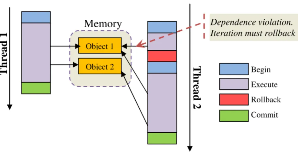
The Optimistic Iteration approach consists of running parallel tasks while assuming that there is no concurrency in data access and that data dependences are maintained throughout the execution. If no race condition occurs, all operations follow regular parallel execution, committing its updates and synchronizing at the end. However, the system makes dependence checks and if a violation occurs, the task that detected the violation is halted and rolled back to its initial state. Upon rollback, every update that task performed on shared objects is undone and the task starts anew. Using transactional semantics helps reduce some of the overheads of lock-based shared-memory synchronization [36]. Fig. 4 shows a small example of Galois’ execution model.
3.1 Galois execution model
The Galois is comprised of three interconnected components: user code, library classes and
24
Programming model
User code is the code a programmer would use to create and manipulate shared objects, expressing a given irregular algorithm. It is based on a programming model that uses set iterators to introduce optimistic parallelism. This approach helps programmers abstract the algorithm from the parallelization concerns and allows parallel algorithms to have sequential-like semantics. The semantic of the set iterators (Fig. 5) is independent of the type of data set being iterated over. This means that the programmer must only concern himself with the algorithm ordering constraints and not with the underlying programming model.
These data sets iterators act as data-oriented worklists in which the order of iteration committal is constrained by the order of the elements in the data set. In case of unordered sets, no particular ordering is enforced. Even if there are dependences among iterations, the result is the same for whichever order the iterations occur. Ordered sets restrict the order of committal to that of the partial ordered set they are iterating. Both sets are unbounded,
Memory
Object 1
Object 2
Dependence violation. Iteration must rollback
T
h
re
a
d
1
T
h
re
a
d
2
Begin
Execute
Rollback
Commit
Fig. 4 – Galois optimistic execution model.
Fig. 5 – Foreach set iterator in Galois. foreach( element in set ){
25
meaning that at any moment during the execution of an iteration a new element can be added to the set.
Galois is based on an object-oriented shared memory model with cache coherence. Direct memory accesses are not allowed and data is accessed by invoking object methods, which is easier for programmers.
Class library
The Galois class library provides method and shared-object implementations to support the implementation of irregular algorithms in Galois. Furthermore, these classes specify how parallel manipulation of object-oriented data can be achieved and provide locality and correctness abstractions for data-structures.
Galois runtime
The runtime of the Galois framework is responsible for issuing iterations to threads and ensuring their subsequent committal or, in case of conflicting iterations, enforcing rollback operations.
3.2 Worklist-based algorithms
Worklists are special data-structures which hold thread-executable units of work, often referred to as tasks. This structure is meant to be accessed in a synchronized way by threads, which retrieve independent tasks and process them concurrently with other task-executing threads. However, in Galois, the runtime system has a scheduler which is responsible for fetching work from the set iterators and creating optimistic parallel iterations. In this instance, set iterators act as data-driven worklists.
Irregular algorithms have two characteristics that make them ideal for implementations using worklist parallelism:
Execution model is centered on iterative processing of data in a loop.
Each iteration might add more elements to the iteration space.
26
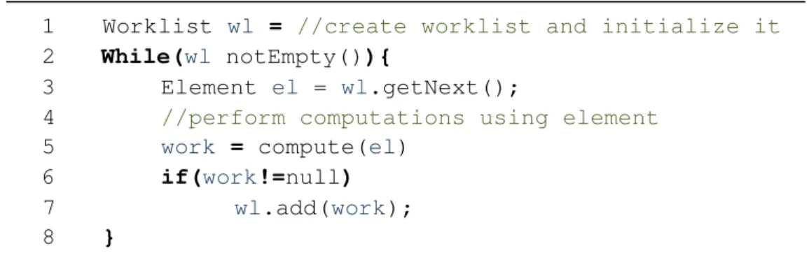
iterations. When an iteration produces more work, a new task is added to the worklist. A pseudo-code example of a basic worklist algorithm can be seen in Listing 1.
3.3 Galois terminology
For a full grasp of the Galois framework, the programmer must understand the abstractions used to separate the actual implementation from the algorithm-specific terminology. In this context, and considering that Galois’ data-structure abstraction is that of a graph, we refer to an active node as the node where computation occurs. The neighborhood of an active node is composed of the set of nodes that are accessed or modified by the active node’s computation.
Fig. 6 shows how these concepts are represented in a graph topology.
The concept of amorphous data-parallelism (section 2.1 stems from this definition as the type of parallelism that can be achieved by parallel processing active nodes subject to neighborhood and ordering constraints. This concept is abstract but it allows us to directly reference parallelism in irregular applications as a special application of general data-parallelism.
Neighborhoods Active Node Non-Active Node
Fig. 6 – Galois abstractions for Irregular algorithms
1 Worklist wl = //create worklist and initialize it 2 While(wl notEmpty()){
3 Element el = wl.getNext();
4 //perform computations using element
5 work = compute(el)
6 if(work!=null)
7 wl.add(work);
8 }
27
4
4
Irregular Algorithms in Galois
In this chapter we shall discuss a few algorithms implemented in Galois so as to provide some insight into some of the concepts previously described. To implement any sort of irregular algorithm in Galois, the programmer must always introduce the following changes to the code:
Use Galois Classes
The Galois Framework provides the programmer with a set of data-structures with which to express the algorithm. These are essentially so that Galois’ runtime is able to recognize how to handle data objects and process the algorithm. These data-structures are implemented around a Graph interface, providing support for directed and undirected graphs, as well as complex, simple and indexed edges. Other shared data-structures and object classes such as a Map, Collection, Set and Accumulator class, provide synchronized runtime logic and are able to be subclassed to suit the user’s needs.
Use Galois Worklists
The Galois framework is directed at worklist implementations of irregular algorithms (as discussed in section 3.2 ), since this is the ideal way in which to explore available amorphous data-parallelism in this type of algorithms. A parallel implementation of an algorithm using a worklist is usually more balanced than other implementations because each thread fetches work as needed. This means that the worst case happens when there is no more work left to be processed but one thread is still processing its task.
28
Use Galois Foreach loops
Galois Iterations require the user to identify the main loops in the algorithm, the ones that guide parallelism, and convert them into foreach loops. As described in programming model in section 0, foreach loops iterate over the elements of the worklist.
Having processed the set of transformations described above, the programmer would eventually reach a base Galois implementation of a worklist algorithm similar to the one depicted in Listing 2.
4.1 Delaunay Triangulation Algorithm
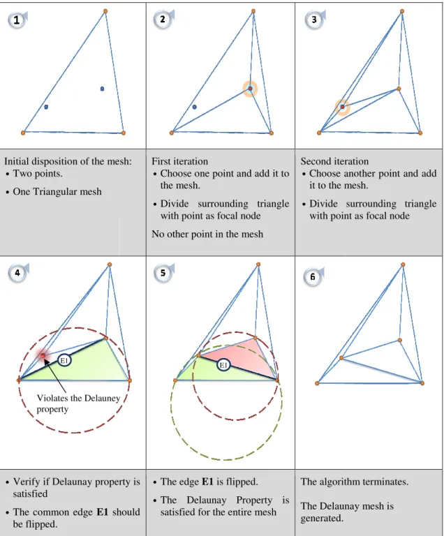
Delaunay’s Triangulation Algorithm [4, 29], also referred to as Delaunay Mesh Generation,
is an algorithm for the generation of a mesh of triangles for a given set of points. In order to generate valid triangulations, every triangle in the generated mesh must fulfill the
Delaunay property. This property states that given a circumference that intersects every triplet of points, no other point belonging to the mesh is located inside the circumference. This algorithm takes an input set of points in 2D space and as a first step surrounds all points with a single triangle. Then, iteratively picks a single point, determines its involving triangle and splits the triangle in three new triangles, with the selected point as focal node. It then follows by checking the Delaunay property and, if it detects a violation, flips the common edge to produce a valid triangulation. An example is given in Fig. 7 and Galois based implementation code is described in Listing 3.
1 Graph g = // initialize with input graph
2 Worklist wl<Elem> = // create worklist of desired type 3 //”Elem” is the type of element that composes a task 4 wl.add( elements ); // populate with initial tasks 5 foreach( Elem e in wl){
6 Elem work = //process e 7 if ( work != null) {
8 wl.add( work);
9 }
10 }
Initial disposition of the mes Two points.
One Triangular mesh
Verify if Delaunay proper satisfied
The common edge E1 sh be flipped.
Fig. 7 – Exam
Implementation in Galois
In Galois, the Delaunay tr
where each node represent triangles. On selecting an a the neighborhood consists flipping activities. Using
E1
Violates the Delauney property
29
esh: First iteration
Choose one point and add it to the mesh.
Divide surrounding triangle with point as focal node
No other point in the mesh
Second iter Choose a it to the m
Divide with poin
erty is
should
The edge E1 is flipped.
The Delaunay Property is satisfied for the entire mesh
The algorit
The Delaun generated.
ample execution of the Delaunay Triangulation alg
is
triangulation algorithm’s mesh is represented nts a triangle and edges represent adjacencies active node, in this case one of the points to ts on the set of triangles affected by the event g triangles as nodes reduces the amount of
E1
ey
teration
e another point and add e mesh.
surrounding triangle oint as focal node
rithm terminates.
unay mesh is
algorithm
30
processing of an active node and reduces the size of the graph while maintaining a tighter coupling of the data dependences.
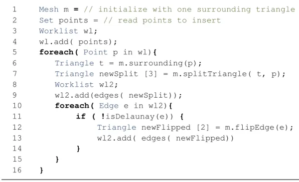
An example of the implementation of this algorithm in Galois is described in Listing 3 and further classification of this algorithm according to the categorization of section 2.1 is summarized in Fig. 8.
Topology Graph (undirected)
Operator type Morph
Ordering Unordered
Fig. 8 – Classification of the Delaunay Triangulation algorithm.
1 Mesh m = // initialize with one surrounding triangle 2 Set points = // read points to insert
3 Worklist wl;
4 wl.add( points);
5 foreach( Point p in wl){
6 Triangle t = m.surrounding(p);
7 Triangle newSplit [3] = m.splitTriangle( t, p);
8 Worklist wl2;
9 wl2.add(edges( newSplit));
10 foreach( Edge e in wl2){ 11 if ( !isDelaunay(e)) {
12 Triangle newFlipped [2] = m.flipEdge(e);
13 wl2.add( edges( newFlipped))
14 }
15 }
16 }
31 4.2 Preflow-push Algorithm
Max-Flow problems [37]consist on finding the maximum flow from a source node to a sink node through a directed graph. Loosely put, this kind of problem can be interpreted as “what is the maximum amount of liquid that can be pumped through a network of pipes”, where the pipes are the edges in the graph. Each edge of the graph has a fixed capacity that represents the maximum amount of flow able to pass through that edge. The general idea underlying this algorithm is that the source is continuously pushing a steady flow to all its downstream neighbors and the flow must find its way to the sink without invalidating the capacity constraints. Furthermore, it has to guarantee that the amount of flow entering a node is equal to the amount of flow leaving that same node – or what is known as flow-conservation property. When no more flow can be pushed in the direction of the sink, the excess flow of a node is pushed back towards the source and must find a new pathway to the sink. There are many algorithms to solve this particular problem, one of which is the Preflow-push algorithm
[33].
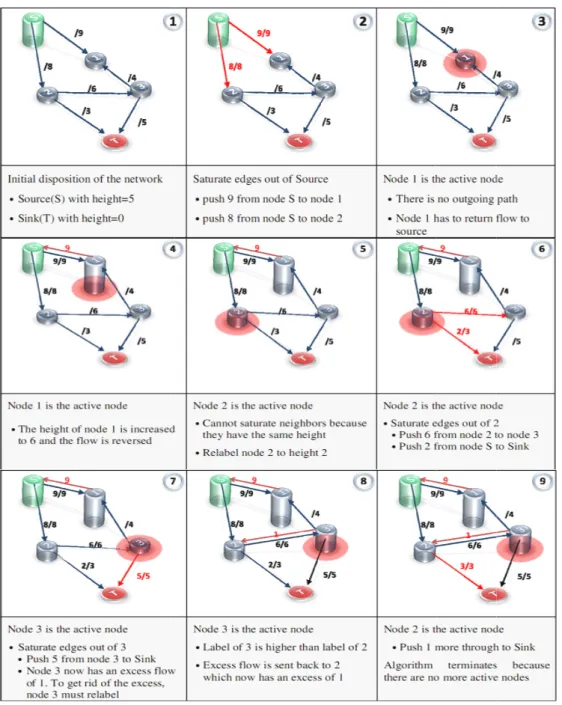
This algorithm’s name derives from the fact that the algorithm does not maintain the flow-conservation property and instead relies on the notion of a preflow, which states that the amount of flow entering a node can at times be more than the total flow leaving that same node. This preflow property defines which nodes have an excess flow and therefore need to be analyzed and processed by the algorithm. Nodes have a hierarchical structure based on a positive height value label, being that the source has height equal to the number of nodes and the sink has height zero. Every other node begins with height equal to one. Throughout the execution of the algorithm, nodes having lower height values are considered to be closer to the sink than its “taller” neighbors. This way, flow is always pushed downstream, in the direction of the sink. Once the algorithm is processing a node, it tries to push flow to a neighboring node that has not reached its total excess capacity and has a lower height value. If there are no valid downstream nodes, then the node is relabeled, that is, its height is incremented until there is at least one available node to which flow can be pushed.
A short example of a complete ex
Fig. 9 – Exam
Implementation in Galois
In Preflow-Push, we define an ac nodes that will be added proces iteration of the foreach then selec Relabel. These conform to a loca values stored by the nodes. For lo
32
execution of the algorithm is shown in Fig. 9.
mple execution of the Preflow-Push algorithm
active node as a node that has some excess flow esses and therefore added to the worklist dyn lects an active node and two activities are perfo
cal computation operator type, in which they locking purposes, the neighborhood of an activ
33
of all its downstream neighboring nodes. Further classification of this algorithm according to the categorization of section 2.1 is summarized in Fig. 10.
Topology Graph (directed)
Operator type Local Computation
Ordering Unordered
Fig. 10 – Classification of the Preflow-Push algorithm.
This behavior is introduced by the Preflowpush class, which provides the base algorithm implementation. An example of this implementation is described in pseudo-code in Listing 4.
1 Worklist wl = new Worklist( graph) //create worklist 2 foreach( Node node: wl){
3 //try to relabel the node
4 graph.relabel( node);
5 //try to push flow to every neighbor
6 for( Neighbor ng : graph.getNeighbors( node)){ 7 if( graph.canPushFlow(node, ng)){
8 graph.pushFlow(node, ng);
9 if ( ! ng.isSourceOrSink())
10 wl.add( ng);
11 if ( ! node.hasExcess())
12 break;
13 }
14 }
15 if ( node.hasExcess())
16 wl.add( node);
17 }
34 4.3 Sparse Cholesky Factorization Algorithm
Cholesky’s factorization [38-39], also known as Cholesky decomposition is a linear algebra method that transforms a matrix into a factor of a unique lower triangular matrix. The general form of this factorization is = , where:
A is a symmetrical positive definite matrix. That is, all it’s diagonal entries are
positive and for every non-zero vector
∈ ℝ
, where denotes the transposematrix
,
> 0
.L is a lower triangular matrix, where by lower triangular matrix we mean a matrix with every entry above the main diagonal equal to zero.
LT is the transpose of the L matrix and therefore an upper triangular matrix with every entry below the main diagonal equal to zero.
As an algorithm, Cholesky has irregular data accesses and traditionally operates on a matrix data-structure, a property it inherits from linear algebra. There are several variations of Cholesky’s factorization but one of the most commonly used, due to its simplicity and the use of sparse matrixes is the Sparse Column-Cholesky factorization algorithm. The column-oriented version of the Cholesky factorization algorithm is shown in Listing 5.
1 Matrix [rows] [columns] m; 2 for ( int col in columns){ 3 for( int row in rows){ 4 if(m [row] [col] != 0)
5 m [] [col] −= m [col] [col] * m [col] [row] * m [] [row];
6 }
7 //divide column m [] [col] by the diagonal
35
Implementation in Galois
Cholesky’s column-oriented algorithm is pretty simple and straightforward but cannot be efficiently parallelized in a data-parallel manner. Therefore, given that the matrix is sparse and can be efficiently mapped onto a graph data-structure, adding the changes described in the beginning of this chapter, one would attain an algorithm identical to the one described in
Listing 6.
In this algorithm, the active nodes are the ones present in the sparse graph, corresponding to the non-zero elements in the original matrix. The neighborhood of the active node is the actual edge neighbors of that same node, except the ones already processes. This is identical to the original algorithm since iterating over the N nodes is equivalent to iterating over the columns of the matrix in the Column-Cholesky version (see Listing 5). Further classification of this algorithm according to the categorization of section 2.1 is summarized in Fig. 11.
1 //get sparse matrix
2 Graph g = //make graph from sparse matrix 3 foreach (Node node in g){
4 //divide column by the “diagonal” 5 for(Edge edge in g.getOutEdges(node)){
6 edge.data /= factor
7 }
8 //divide edges by a factor
9 for(Node node2 in neighbors(node)){
10 for(Node node3 in neighbors(node)){
11 edge = g.getEdge (node2, node3);
12 if((node2==node3) and notSeen(edge)){
13 //same as m [] [col]−= m [col] [col]* m [col] [row]* m [] [row];
14 v2 = g.getEdge(node,node2).value;
15 v3 = g.getEdge(node,node3).value;
16 edge.data −= v2*v3;
17 }
18 }
19 }
20 //Add result to answer Graph
36
Fig. 11 – Classification of the Sparse Cholesky Factorization algorithm.
4.4 Kruskal’s Minimum Spanning Tree Algorithm
Kruskal’s algorithm [37] finds minimum spanning trees(MST), that is, given a graph it finds a tree that is composed of a set of edges such that:
Every node in the graph is connected to at least one edge in the set.
The total weight of the set of edges is less than or equal to the total weight of every other possible spanning tree.
Kruskal’s MST is a special case of a more general problem called the union-find problem [40]. A union-find is a data-structure that represents a set of disjoint non-empty sets. There is a wide variety of implementations for the Kruskal’s MST problem, but we shall only refer to the union-find implementation variant.
The general conceptualization of this algorithm first creates a union-find and populates it with the nodes in the graph, on disjoint non-empty set for each node. The edges of the graph are then placed in a priority queue, ordered by increasing edge weight. The algorithm then follows by iterating over an ordered queue containing every edge in the graph, in order of increased weight. In every iteration, the edge with the lowest weight is removed from the queue and if its connecting nodes belong to different sets, both sets are joined by creating an edge between those nodes in the union-find. If the nodes already belong to the same set, the edge is discarded and a new iteration commences. When all edges have been removed from the queue, the algorithm completes and the union-find now represents the minimum spanning tree of the original graph.
Topology Graph (undirected)
Operator type Reader ( in relation to the input graph)
Morph (in relation to the output graph)
37
Galois implementation
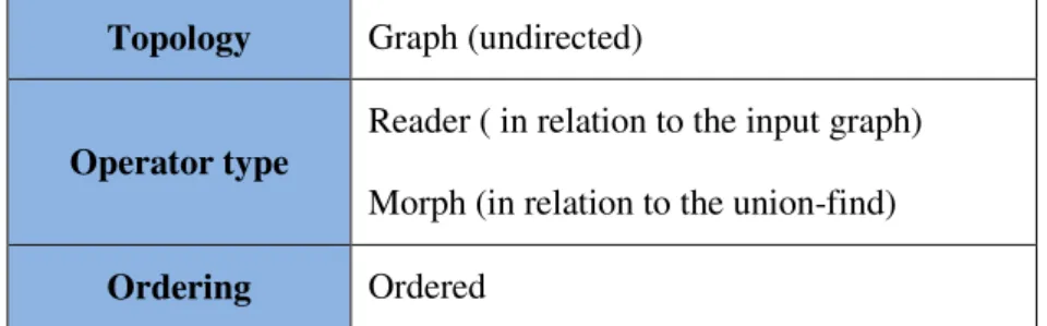
In the Galois implementation of this algorithm, active elements are the edges of the graph, represented in an ordered worklist. For each iteration, the neighborhood of an active edge is composed of its connected nodes and all elements in the sets to whom the nodes. The union-find can be created by subclassing or wrapping one of the provided set of Galois graph classes. An example of the implementation of this algorithm in Galois is described in Listing 7 and further classification of this algorithm according to the categorization of section 2.1 is summarized in Fig. 12.
Topology Graph (undirected)
Operator type
Reader ( in relation to the input graph) Morph (in relation to the union-find)
Ordering Ordered
Fig. 12 – Classification of Kruskal’s MST algorithm.
1 Graph g = // read in graph 2 MST mst = new MST( );
3 UnionFind uf = new UnionFind(); 4
5 foreach( Node n in g ){
6 uf.create(n);//create new set 7 }
8 foreach( Edge e in g ){//ordered by weight 9 Node n1 = e.getHead();
10 Node n2 = e.getTail();
11 if( uf.find(n1)!=uf.find(n2)){ 12 uf.union(n1,n2) ;
13 mst.add(e);//put e in MST
14 }
15}
38
39
5
5
Arclight Plugin
Paramount to the task of identifying the concurrency patterns in the Galois framework, was the analysis of just how much Galois-specific code was present in the implemented algorithms. Our proposal was to identify the different concerns present in Galois implementations of algorithms and measure the amount of tangling present. A concern, according to Robbillard [41] is any type of special consideration about the software being implemented. In this case, we identified a set of five code concerns related to Galois: Algorithm code, Galois prologue code, Galois epilogue code, Galois interlogue code and Miscellaneous code.
Algorithm code concerned the actual algorithm structure, whether implemented in Galois or in whichever other framework or language. The Galois-specific data-structures was also regarded as belonging to this concern since they only replace the previous data-structures.
Galois prologue code concerned code that was needed to instantiate and initialize a Galois implementation.
Galois epilogue codeconcerned post-algorithmic operations. The majority of this type of code concerned result verification code which was in fact irrelevant for the task at hand and so this code was also tagged as miscellaneous code.
Galois interlogue code concerned Galois specific code that was interleaved with algorithmic code. This usually meant optimization related code.
Miscellaneous code concerns non-essential code, such as comments, variable declaration, etc.
Six concern exploration tools were considered to the task of marking and exploring the concerns in the code of Galois algorithms: FEAT [42], ConcernMapper [43], Sextant [44],
40
concern identification, with varying degrees of efficiency, none presented the capability to extract metrics from the concerns.
To this task, ArchLight, an eclipse code tagging plugin, was implemented. This plugin consisted on a specialized toolbar (Fig. 13) that allowed the coloring of different concerns present in the code and the application of sizing metrics.
The plugin consisted in a toolbar that allowed us to colorize the code according to five types of concerns present in the set of Galois algorithms’ code.
Fig. 13 – ArchLight plugin toolbar.
Fig. 14 shows how the correspondence between the coloring and the different concerns was accomplished.
Fig. 14 – ArchLight Eclipse Plugin concern coloring. Algorithm Code
Galois prologue code
Miscellaneous code
Galois epilogue code
41
This tagging of the code allowed us to retrieve some sizing metrics (Fig. 15) to evaluate the percentage of code available for the identification of the patterns. This procedure was performed on four of the fourteen algorithms currently implemented using Galois. The algorithms analyzed are described in chapter 4. The results achieved are summarized in
Fig. 16. These results were achieved by a measure of the number of lines of source code (LoC) per code concern, disregarding comments, empty and single character lines. A total of 2024 lines of code where analyzed.
Fig. 16 – Percentage of Galois code in the code of irregular algorithms
Algorithm Prologue Interlogue Misc
Average Percentage of code 63% 2% 1% 34%
Average Percentage of code
(without miscellaneous code) 95% 3% 2% 0%
42
These results led us to believe that the amount of code directly related to Galois is very small indeed, on an average of 5% of the total LoC written for a given algorithm. The absolute number of LoC varies according to the complexity of the algorithm but in the implementations analyzed, this was on average a mere three to five lines of code per class. This in turn meant that the amount of available code to extract patterns was indeed limited and therefore the number of patterns able to emerge is also limited.
43
6
6
Patterns and Pattern Languages
Over the last 30 years, the field of software development has been evolving at an accelerated rate. New and progressively more advanced techniques arise on a daily basis to the point that it is no single person can hope to grasp the existing volume of knowledge on software construction. Nowadays, the number of available software development techniques is so immense that programmers are ever more focused on small, specific areas of the software domain. Deciding on a specific methodology and development strategy with which to implement an algorithm is almost impossible and programmers often opt to use the solution they know best, even if it is not optimal. Thus, in order to reuse good software development practices and techniques, it is essential that expert programmers identify and document the best practices in their specific domain. In this context, Software Patterns represent well-documented template solutions that can be reused whenever a certain problem arises in a well-known context [6].
6.1 Patterns
For years, software developers had to rely on their own knowledge and intuition to understand which solutions were available and to decide which of those was the ideal solution for a specific problem. This meant that programmers had to be versed in a multitude of domains and methodologies, from different paradigms, frameworks and languages, to programming libraries, algorithms, databases, web and networks, parallel programming, compilation, hardware architecture, etc. The list is immense and the sheer amount of knowledge required to have even a broad overview of all these subjects takes years of study and dedication. Patterns help to reduce this effort.
44
For a pattern to be accepted by the community as representing a valid solution, the knowledge it conveys should be widely recognized as being mature and complete representations of a tangible solution to a problem that arises in a well defined context within a specific domain. Therefore, patterns must be concrete enough so as to represent valid solutions, yet their context should be relaxed enough to allow their application to a variety of problems.
The idea of describing reusable problem solutions as patterns first arose in the beginning of the 1970s in the domain of architecture and as a form of capturing solutions to common design problems on the construction of buildings and towns [48]. Alexander, the architect and author of the idea, latter coined the term “Pattern” to describe what he deemed to be “a perennial solution to a recurring problem within a building context, describing one of the configurations which brings life to a building.”
In the software development community, patterns were first introduced by Beck and Cunningham [49] in 1987. However, the true impact of patterns for software development only became apparent when, in 1995, Gamma, Helm, Johnson, and Vlissides published a book containing 23 software design patterns. The book was so widely accepted that Gang of Four, i.e. the four authors, quickly became synonym with software design patterns. Design patterns represent design problems and their respective solutions and entail cooperation between classes and object. These represent only a subset of the overall set of software patterns since they do not consider computational problems such as algorithms or structural problems such as parallelism and distribution [50]. After the popularity of the Gang of Four patterns, pattern-oriented software development became a prolific area in the domain of software development. Patterns spawn multiple application domains such as object-oriented programming [7], aspect-oriented programming [8] framework design [9-10], software architecture [11-12], components [13], machine learning [14-15] and even patterns about patterns [16-17].
45
references various software pattern collections and accounts for over 2900 patterns1. Others are more focused, like the Hypermedia Design Patterns Repository [52] or the Human-Computer Interaction and User Interface Design pattern repository [53]. PatternForge, a wiki for the EuroPLoP 2007 Focus Group on Pattern Repositories, lists 29 pattern repositories available on the web [2, 54].
6.2 Pattern languages
When patterns are considered in isolation, as single entities, software developers cannot be fully aware of how the pattern was originally intended to be composed with other patterns. Using stand-alone patterns for real-world systems frequently results in added an increase in design complexity, since single patterns cannot consider the multifaceted context of large scale software [55].
Pattern catalogues should therefore be introduced as Pattern Languages, which consider pattern dependences and guide pattern-oriented software development. Pattern languages form complete sets of patterns, such that choosing to use one pattern will eventually direct the software developer to use another related pattern. Following the sequence of pattern dependences will lead to a complete solution for a complex context.
However, there is no formally defined rule for defining pattern dependences in pattern languages. Dependences are usually introduced by a graphical mapping of dependences [56-57] or, more traditionally, through a Related Patterns section in the body of the pattern [6]. Graphical descriptions of the dependences between patterns are very useful to provide an overview of how patterns interact. However, they only present short non-descriptive commentaries. A Related Patterns section is more verbose but can often be interpreted in slightly different ways. Therefore, most modern pattern languages use a composition of both forms since they are complementary [58].
Independently of the recognized benefits of using pattern languages, there are still significantly more independent patterns than complete languages. Booch recently presented a study that identified 1938 patterns, collected from a set of 1884 individual patterns and only
1
46
54 pattern languages [59]. This fact proves that there is still much work to be done in the field of pattern languages for software development.
6.3 Form and Style
There is no consensus on the formal structure of pattern description and many authors coin their own format. The main templates of pattern description relate to Alexandrian form [48], Gang of Four form [6] and Coplien form [17]. In Alexandrian patterns, the general form and style includes pattern name, context, main (problem statement, forces, solution instruction, solution sketch, solution structure and behavior), and consequences. The Gang of Four design patterns presents a structure composed of Pattern Name and Classification, Intent, Also Known As, Motivation, Applicability, Structure, Participants, Collaborations, Consequences, Implementation, Sample Code, Known Uses, and Related Patterns. Coplien Patterns are based on Alexandrian form but present patterns in a reduced format, which includes Pattern Name, Problem, Context, Forces , Solution, Rationale, Why does this pattern work? and Resulting Context.
There are several other forms for pattern description in use by the pattern community. However, in general, there are five elements that are consistent in the various formats: pattern name, problem description, context, forces and solution.
Pattern name
The name of the pattern needs to convey a sense of the purpose of the pattern and are usually used as substantives in the body of the pattern.
Problem description
This section describes the essential information about the problem the pattern proposes to solve. It is usually a small paragraph where the author states the question that conveys the problem.
Context
47
preconditions or consideration, while at the same time allowing it to be applicable to various contexts.
Forces
Forces represent constraints and decisions and are often described in pairs of opposing considerations, tradeoffs or compromises. The forces section is not standardized among the various authors.
Solution
48
Amorphous
Data-Parallelism
Optimistic Iteration
Data-Parallel
Graph
7
7
Pattern Language
In this section, the pattern language.
The pattern language is s implementation of an irregu It intends to be as general patterns found in Galois, its overview of the pattern lang
Fig.
49
Graph Partitioning
Graph Partition Execution Strategy
In-Order Iteration
Iterat
Lock
Pree
ge
rns found within the Galois Framework are d
structured so as to separate the various co gular algorithm in an amorphous data-parallel ral as possible, and although its main object its usefulness is not specifically limited to the G
nguage is shown in Fig. 17.
ig. 17 – Overview of the Pattern Catalogue.
One Shot
eration Chunking
Lock Realocation
reemptive Read
e described as a pattern
50
The design of the pattern language follows a hierarchical structure that represents the order in which these sets of patterns should be applied, that is, execution patterns intuitively build upon the structural patterns implementation and optimization patterns build upon execution patterns. The implementation steps are congruent with the actual considerations that the programmer must take when deciding to implement an irregular algorithm and are divided into three separate sets:
1. Structural patterns consider how to structure irregular algorithms in terms of their algorithmic properties and data-structures and how these will be affected by optimistic parallel execution. This set of patterns is the most important of the pattern language, since the two underlying design spaces build directly upon its properties. If the programmer cannot conform to these patterns, then using patterns from this language is discouraged.
2. Execution patterns effectively take into account how the actual execution of the algorithm is handled and how to guide the algorithm to explore the maximum amount of parallelism. Not taking these patterns into consideration may lead to lower performance benchmarks.
3. Optimization patterns are designed to present the final phase of implementation and essentially focus on some optimizations that, when applied over structural patterns, contribute to further increase the performance of irregular parallel algorithms.
In this sense, this pattern language is meant to be applied as a sequence of steps that will eventually transform an irregular algorithm into a Galois parallel irregular application. However, there are some considerations as to the actual application of the patterns since there are relationships and dependences among them that might provide further insight to the applicability of a pattern at a given moment. The diagram of Fig. 18 further describes these relationships.
Note that this is in fact a conservative representation of the relationships among patterns and not every relationship is explicitly represented as an arrow – the different levels of the patterns also imply dependences. Every optimization and execution pattern requires the application of structural patterns and, while their implementation is not strictly necessary,
of dependences among pat pattern.
Fi
This tight dependence bet language and not a mere cat
51
patterns shall be referred to in the related pat
Fig. 18 – Explicit relationships among patterns.
etween patterns is a clear indicative that thi catalog.
patterns section of each
52
The form and style used for the pattern language builds upon the pattern name- problem-description-context-forces-solution form, described in section 6.3 , and includes the Also Known As, Galois Implementation, Example, Related Patterns and Known Uses sections:
Also Know As – presents several alternative names, representing the same concept but directed at different domains or methodologies.
Galois Implementation – in this section we present some concepts of how this patter is implemented in the Galois Framework. It is complementary to both the Solution and the Example sections since it presents a case study of how the pattern can be applied.
Example – the examples section validates the pattern by using it to solve a well known problem.
Related Patterns – this section presents small textual descriptions of dependences the pattern has with other patterns in the same pattern language or with external patterns.
Known Uses – together with the example section, this section validates the pattern by demonstrating its use in the software development community.
7.1 Pattern Terminology
In order to help the reader abstract from algorithm and implementation specific jargon, we describe in this section some of the more general terms used in our pattern language:
Available parallelism – number of iterations available for concurrent execution at any single instance in time.
Data element – a data element is a well-identified, describable unit of data that may be indivisible or consist of a set of data items. Additionally, data elements can be individualized from the overall data set. The identification of such data elements is algorithm-specific and usually comprises on an often repeated name whose meaning is associated to the algorithmic metaphor. Using examples of the previously described algorithms, for the Preflow-push Algorithm (section 4.2 a data element is a node on the path from source to sink, while on Delaunay Triangulation Algorithm (section 4.1 the data element is a triangle on the mesh.
53
Iteration – an iteration represents the unit of a step in the solution of an algorithmic problem. To solve an algorithm implies repetitively applying that step a finite number of times, i.e., to iterate an algorithm is to repeatedly apply the same operation over a set of data until de algorithm terminates. Moreover, often it involves using the output of an iteration as the input of its predecessor.
Work – a work element is equivalent to an iteration since when processing iterative work-list based algorithms, the element that is retrieved from a worklist represents an iteration of the algorithm.
Set of neighbors or neighborhood – represent the set of data elements will be read or written by a computation.
Processing Unit – represents either a processor core or thread and is used to abstract from the actual processing element. Therefore, our patterns can be used in both multi-core and multi-threaded environments.
7.2 Algorithm Structure Patterns
7.2.1 Amorphous Data-Parallelism
Problem
How to exploit concurrency in the presence of unpredictable data dependences?
Context
Traditional data parallelism exploits the decomposition of data-structures as a way to attain concurrent behavior. This entails dividing the data structure into independent sets and distributing them among processing units in a way that allows for the parallel application of a stream of operations.
54
Amorphous data-parallelism is a particular form of data-parallelism that arises when the underlying data-structure has no fixed shape or size, i.e. is amorphous, implying that the amount of available opportunities for concurrency-free parallelism is unpredictable.
How then can we decompose an algorithm’s data in a way that allows for data-parallel execution, when:
1. The occurrence and location of data accesses can only be properly estimated at runtime.
2. Concurrent computations may modify the structure of underlying data.
Forces
Data Granularity
Coarse-grained data may imply less communication but will introduce larger computational overhead and reduce the amount of available parallelism opportunities. If on the other hand the grain is fine, communications will represent the major overhead but will introduce a greater amount of available parallelism.
Redundancy vs. Communication
In a distributed environment, it can be profitable to perform redundant calculations in each of the distribution locales, instead of relying on data communication. This can introduce scalability opportunities.
Sequential to Parallel Traceability
If the pattern is well applied, there must be a simple and convenient mapping between the sequential and parallel versions of an implementation. This allows programmers to easily check the correctness of their implementation.
Modifications to the data-structure do not create deadlock opportunities.
Solution
55
As such, the general solution for this problem entails being able to, at each iteration:
1. Identify the independent sets of data able to be executed in parallel
2. Decide which shared data elements need to be locked to avoid concurrent access
3. Ensure that the computational cost of independent sets remain balanced
Also, a decomposition based on amorphous data-parallelism must ensure that:
Data dependent computations drive parallelism.
Computations are performed in a way that introduces opportunities for independent parallel execution over the data.
The general solution of this pattern is comprised of the following steps:
S
Stteepp11--Determine the type of algorithm operator
Following the characteristics described in Categorization of irregular algorithms2.2
(section 2.3) the operator of an algorithm can be one of three types: Morph, Local Computation and Reader.
The semantics of the operator is defined by degree of influence:
Morph algorithms have at least one morph operator.
Local Computation algorithms have no morph operator and at least one local computation.
Reader algorithms have strictly reader operators.
S
Stteepp22--Define a valid data-parallel decomposition based on the concept of basic data element