Regional Extinctions and Quaternary Shifts in
the Geographic Range of
Lestodelphys halli
,
the Southernmost Living Marsupial: Clues for
Its Conservation
Anahí E. Formoso
1*
, Gabriel M. Martin
2, Pablo Teta
3, Aníbal E. Carbajo
4,
Daniel E. Udrizar Sauthier
5, Ulyses F. J. Pardi
ñ
as
11Instituto de Diversidad y Evolución Austral (CONICET), Puerto Madryn, Chubut, Argentina,2Laboratorio de Investigaciones en Evolución y Biodiversidad, Facultad de Ciencias Naturales, sede Esquel, Universidad Nacional de la Patagonia San Juan Bosco, Esquel, Chubut, Argentina,3División Mastozoología, Museo Argentino de Ciencias Naturales“Bernardino Rivadavia”, Avenida Ángel Gallardo 470, C1405DJR, Buenos Aires, Argentina,4Ecología de Enfermedades Transmitidas por Vectores, Instituto de Investigación e Ingeniería Ambiental, Universidad Nacional de San Martín, San Martín, Buenos Aires, Argentina,5Instituto Patagónico Para el Estudio de Ecosistemas Continentales (IPEEC) and Facultad de Ciencias Naturales, sede Puerto Madryn, Universidad Nacional de la Patagonia“San Juan Bosco”, Puerto Madryn, Chubut, Argentina
*formoso@cenpat-conicet.gob.ar
Abstract
The Patagonian opossum (
Lestodelphys halli
), the southernmost living marsupial, inhabits
dry and open environments, mainly in the Patagonian steppe (between ~32°S and ~49°S).
Its rich fossil record shows its occurrence further north in Central Argentina during the
Qua-ternary. The paleoenvironmental meaning of the past distribution of
L
.
halli
has been mostly
addressed in a subjective framework without an explicit connection with the climatic
“
space
”
currently occupied by this animal. Here, we assessed the potential distribution of this
spe-cies and the changes occurred in its geographic range during late Pleistocene-Holocene
times and linked the results obtained with conservation issues. To this end, we generated
three potential distribution models with fossil records and three with current ones, using
MaxEnt software. These models showed a decrease in the suitable habitat conditions for
the species, highlighting a range shift from Central-Eastern to South-Western Argentina.
Our results support that the presence of
L
.
halli
in the Pampean region during the
Pleisto-cene-Holocene can be related to precipitation and temperature variables and that its current
presence in Patagonia is more related to temperature and dominant soils. The models
obtained suggest that the species has been experiencing a reduction in its geographic
range since the middle Holocene, a process that is in accordance with a general increase in
moisture and temperature in Central Argentina. Considering the findings of our work and
the future scenario of global warming projected for Patagonia, we might expect a harsh
impact on the distribution range of this opossum in the near future.
a11111
OPEN ACCESS
Citation:Formoso AE, Martin GM, Teta P, Carbajo AE, Sauthier DEU, Pardiñas UFJ (2015) Regional Extinctions and Quaternary Shifts in the Geographic Range ofLestodelphys halli, the Southernmost Living Marsupial: Clues for Its Conservation. PLoS ONE 10(7): e0132130. doi:10.1371/journal.pone.0132130
Editor:Peter Wilf, Penn State University, UNITED STATES
Received:May 7, 2015
Accepted:June 10, 2015
Published:July 23, 2015
Copyright:© 2015 Formoso et al. This is an open access article distributed under the terms of the
Creative Commons Attribution License, which permits unrestricted use, distribution, and reproduction in any medium, provided the original author and source are credited.
Data Availability Statement:All relevant data are within the paper and its Supporting Information files.
Funding:This research was funded by Consejo Nacional de Investigaciones Científicas y Técnicas and Agencia Nacional de Promoción Científica y Tecnológica (PICT 2008-547 to UFJP).
Introduction
The Patagonian opossum,
Lestodelphys halli
[
1
], is endemic to Argentina and the southernmost
living marsupial. Its current range extends from 32.5° S (North of Mendoza Province) to 48.6°S
(center of Santa Cruz Province), showing an almost continuous distribution through southern
Río Negro and Chubut and Santa Cruz Provinces (40° S to 48.6° S), and including a few and
isolated records, widely scattered between 32.5°S and 39.5°S (Mendoza, La Pampa and
north-ern Río Negro Provinces [
2
–
5
]). In a phytogeographic context,
L
.
halli
inhabits the Patagonian
steppe almost exclusively, although sparse records throughout the Monte desert have been
found [
2
,
3
,
6
,
7
]. Our knowledge on the distribution of this marsupial has greatly increased
during the last two decades. For more than 65 years,
L
.
halli
was only known from nine
speci-mens from three localities in Chubut and Santa Cruz Provinces [
8
] and was considered as one
of the most poorly known mammals in the world [
6
,
8
,
9
]. In contrast, by the end of the 1990's,
this species had been reported in more than a dozen localities [
6
,
9
], mainly recovered from
owl pellet analyses [
2
,
5
,
7
,
10
–
12
]. These findings changed our perception of this opossum
from considering a rare to a moderately common species of the extra-Andean small mammal
community. These new records demonstrated that this species had been largely overlooked,
probably because of its low capture rate with traditional traps [
5
,
13
].
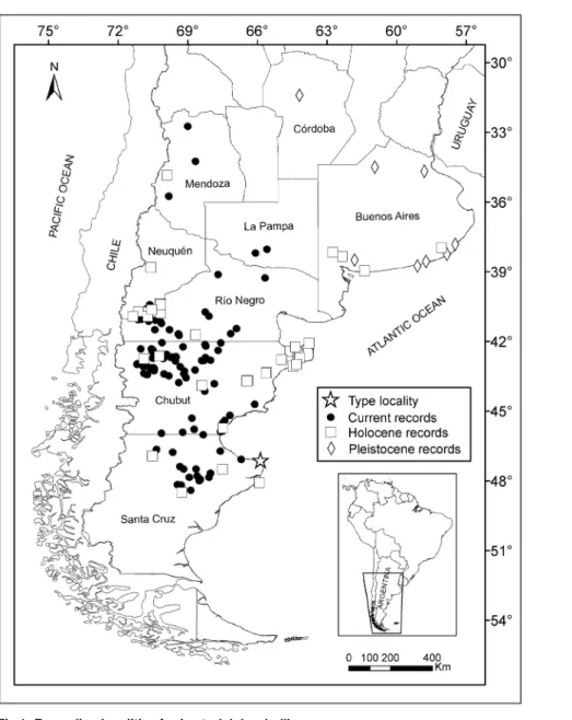
Contrasting with most living South American marsupials,
Lestodelphys halli
inhabits dry
and open environments in southern South America (
Fig 1
) [
5
,
14
] and also has a rich
paleonto-logical record [
15
–
17
]. Fossils show that the species lived in most of the Patagonian and
Pam-pean regions during the Quaternary, reaching Central Argentina as far north as 32° S [
2
,
15
,
18
–
20
]. Its extra-limital records have been interpreted as indicators of hostile climatic
condi-tions during the Pleistocene and most part of the Holocene [
15
,
16
,
21
–
23
]. However, the
paleoenvironmental meaning of the species' fossil record has been mainly addressed in a
sub-jective framework, without a formal connection to the climatic
“
space
”
currently occupied by
this animal [
15
,
16
,
24
].
The aim of this study was to assess the past and current potential distributions of
L
.
halli
in
order to test more accurately their significance as a proxy for cold and dry climatic conditions
in the Southern cone of South America. To this end, we identified the most important
environ-mental variables that explain the species
’
distribution and inferred the possible causes of
regional extinctions and shifts. We also discuss conservation issues, particularly taking into
account that the species has been suffering a reduction in its geographic range since the middle
Holocene and the future warming that is affecting its range.
Materials and Methods
The current records of
Lestodelphys halli
used to generate our models were retrieved from
trapped specimens, owl pellets, museum specimens and the literature [
5
,
7
,
11
,
12
]. Trapped
specimens and those recovered from owl pellets are housed at Colección de Material de
Egagró-pilas y Afines
“
Elio Massoia
”
(CNP-E) and Colección de Mamíferos (CNP), both from Centro
Nacional Patagónico, Puerto Madryn, Chubut, Argentina; Museo Argentino de Ciencias
Natur-ales
“
Bernardino Rivadavia
”
(MACN), Ciudad Autónoma de Buenos Aires, Argentina; and
Laboratorio de Investigaciones en Evolución y Biodiversidad (LIEB), Universidad Nacional de
la Patagonia San Juan Bosco, Esquel, Chubut, Argentina. The paleontological data used to
gen-erate our models were based on the fossils collected in the field and records retrieved from the
literature [
15
,
17
,
21
]. The fossils collected were housed at CNP-E. Permits for collection were
given by the Ministerio de Comercio Exterior, Turismo e Inversiones, Subsecretaría de Turismo
y Áreas Protegidas de la provincia del Chubut, Argentina (number 209-SSTyAP/08).
Fig 1. Recording localities forLestodelphys halli.
Localities in which the species was recorded were divided into
“
current localities
”
, which
included records from 1921 (when
Lestodelphys halli
was named) to the present, and
“
fossil
localities
”
, which included records from the Pleistocene (~2.59 million years before present) to
the late Holocene (i.e., up to ~200 years before present). As part of the Pleistocene records, we
also included those referred to
†
Lestodelphys juga
[
30
], a taxon alternatively considered as valid
[
2
,
21
] or suggested as a junior synonym of
L
.
halli
[
17
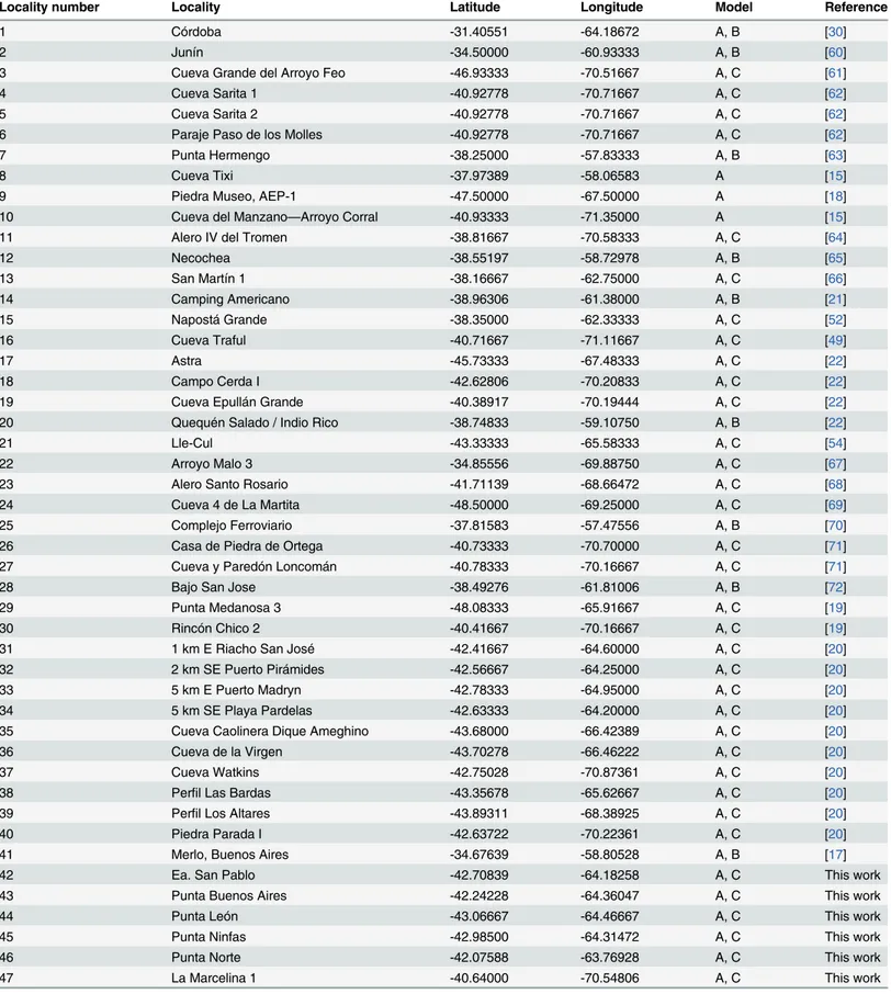
]. We accounted for 47 fossil localities
(
Table 1
) and 124 current localities (
Table 2
). Fossil records included nine from the Pleistocene
and early Holocene, 35 from the middle and late Holocene, and three that could not be
assigned to any age in particular (i.e., Cueva Tixi, Piedra Museo and Cueva del
Manzano-Arroyo Corral;
Table 1
). These localities belong to the Holocene sensu lato; they were excluded
from the models because they lacked an accurate age and could not be allocated to any of the
three divisions of the Holocene [
15
,
18
].
We generated six potential distribution models using MaxEnt software 3.3.3e version [
31
]:
three with fossil records and three with extant records. Localities used to generate the fossil
models were divided into: All-fossils, including all fossil records from the Pleistocene and
Holocene; Last Glacial Maximum (LGM), including records from the Pleistocene and
early Holocene; and middle to late Holocene (M/L Holocene), including fossil records from
6000 to 200 years before present. Localities used to generate the current models were
divided into: All-current, including all known records from the species description in 1921 to
2013; 1950, including records from 1950 to 2013; and 1950
–
2000, including localities
recorded from 1950 to 2000, in strict accordance with the WorldClim environmental layers
(see below). Environmental layers used in the generation of these models included three
dif-ferent databases. The first database included 19 bioclimatic variables from the LGM (~21000
years before present). These are biologically meaningful variables derived from monthly
aver-age temperature and rainfall values, with a spatial resolution of 2.5 arc-minutes and based on
the Paleoclimate Modeling Intercomparison Project Phase II; PMIP
2,
http://pmip2.lsce.ipsl.
fr/
[
32
]. The second database included 19 bioclimatic variables, monthly average minimum
and maximum temperatures and monthly total precipitation from the middle Holocene;
CCSM4 [
33
] with a spatial resolution of 30 arc-seconds. The third database included
World-Clim variables (1.4 version;
www.worldclim.org
) for current climate (from 1950 to 2000),
with a spatial resolution of 30 arc-seconds [
34
]. This set comprised monthly average
mini-mum, mean and maximum temperatures, monthly precipitation, altitude and 19 bioclimatic
variables.
We added four categorical variables to the analyses of current localities: global vegetation
coverage (globcov), land-form, dominant soil (dominant soil type) and parent material
(par-entmat; i.e., the material from which soil develops). These variables are from the SOTERLAC
database [
35
] and they incorporated landscape and soil information to the analyses which is
not contained in the climatic variables.
The following setup was used for all models: logistic output format, 25% of the records used
as training data, 1000 iterations, 10000 background points (randomly selected by MaxEnt) and
random seed. The logistic output format was used assigning values of probability of presence
to the models, with the following colors: 0.5
–
1 (red), 0.25
–
0.5 (orange), 0.1
–
0.25 (yellow),
0.02
–
0.1 (green) and 0
–
0.01 (white). The background point values (i.e., 10000) were selected to
Table 1. Fossil localities forLestodelphys halli.
Locality number Locality Latitude Longitude Model Reference
1 Córdoba -31.40551 -64.18672 A, B [30]
2 Junín -34.50000 -60.93333 A, B [60]
3 Cueva Grande del Arroyo Feo -46.93333 -70.51667 A, C [61]
4 Cueva Sarita 1 -40.92778 -70.71667 A, C [62]
5 Cueva Sarita 2 -40.92778 -70.71667 A, C [62]
6 Paraje Paso de los Molles -40.92778 -70.71667 A, C [62]
7 Punta Hermengo -38.25000 -57.83333 A, B [63]
8 Cueva Tixi -37.97389 -58.06583 A [15]
9 Piedra Museo, AEP-1 -47.50000 -67.50000 A [18]
10 Cueva del Manzano—Arroyo Corral -40.93333 -71.35000 A [15]
11 Alero IV del Tromen -38.81667 -70.58333 A, C [64]
12 Necochea -38.55197 -58.72978 A, B [65]
13 San Martín 1 -38.16667 -62.75000 A, C [66]
14 Camping Americano -38.96306 -61.38000 A, B [21]
15 Napostá Grande -38.35000 -62.33333 A, C [52]
16 Cueva Traful -40.71667 -71.11667 A, C [49]
17 Astra -45.73333 -67.48333 A, C [22]
18 Campo Cerda I -42.62806 -70.20833 A, C [22]
19 Cueva Epullán Grande -40.38917 -70.19444 A, C [22]
20 Quequén Salado / Indio Rico -38.74833 -59.10750 A, B [22]
21 Lle-Cul -43.33333 -65.58333 A, C [54]
22 Arroyo Malo 3 -34.85556 -69.88750 A, C [67]
23 Alero Santo Rosario -41.71139 -68.66472 A, C [68]
24 Cueva 4 de La Martita -48.50000 -69.25000 A, C [69]
25 Complejo Ferroviario -37.81583 -57.47556 A, B [70]
26 Casa de Piedra de Ortega -40.73333 -70.70000 A, C [71]
27 Cueva y Paredón Loncomán -40.78333 -70.16667 A, C [71]
28 Bajo San Jose -38.49276 -61.81006 A, B [72]
29 Punta Medanosa 3 -48.08333 -65.91667 A, C [19]
30 Rincón Chico 2 -40.41667 -70.16667 A, C [19]
31 1 km E Riacho San José -42.41667 -64.60000 A, C [20]
32 2 km SE Puerto Pirámides -42.56667 -64.25000 A, C [20]
33 5 km E Puerto Madryn -42.78333 -64.95000 A, C [20]
34 5 km SE Playa Pardelas -42.63333 -64.20000 A, C [20]
35 Cueva Caolinera Dique Ameghino -43.68000 -66.42389 A, C [20]
36 Cueva de la Virgen -43.70278 -66.46222 A, C [20]
37 Cueva Watkins -42.75028 -70.87361 A, C [20]
38 Perfil Las Bardas -43.35678 -65.62667 A, C [20]
39 Perfil Los Altares -43.89311 -68.38925 A, C [20]
40 Piedra Parada I -42.63722 -70.22361 A, C [20]
41 Merlo, Buenos Aires -34.67639 -58.80528 A, B [17]
42 Ea. San Pablo -42.70839 -64.18258 A, C This work
43 Punta Buenos Aires -42.24228 -64.36047 A, C This work
44 Punta León -43.06667 -64.46667 A, C This work
45 Punta Ninfas -42.98500 -64.31472 A, C This work
46 Punta Norte -42.07588 -63.76928 A, C This work
47 La Marcelina 1 -40.64000 -70.54806 A, C This work
Table 2. Current localities forLestodelphys halli.
Locality number
Locality Latitude Longitude Model Reference
1 Cabo Tres Puntas -47.10000 -65.86 A [1]
2 Pico Salamanca -45.40000 -67.40000 A [73]
3 Ea. Los Manantiales -43.40000 -70.01667 A [74]
4 Choele Choel -39.26667 -65.66667 A, B, C [75]
5 2 km NNW RN 40 y RP 237 -40.41667 -70.63333 A, B, C Pearson O. Field notes 1982–1983:
79 (MVZ Library)
6 Cerro Leones -41.06667 -71.13333 A, B, C [76]
7 Cañadón Las Coloradas, Alm. El Manzano -40.65000 -70.78333 A, B, C [77]
8 Pampa de Nestares -40.58333 -70.75000 A, B, C [78]
9 Cerro Castillo (= Guacho), Paso Flores -40.58333 -70.66667 A, B, C [79]
10 10 km E Clemente Onelli -41.16667 -70.16667 A, B, C [6]
11 10 km WSW Comallo -41.50000 -70.41000 A, B, C [6]
12 15 km SE Los Menucos -40.91667 -68.08333 A, B, C [6]
13 Chacras de Coria -32.75000 -69.00000 A, B, C [6]
14 Ea. Tehuel Malal -41.03333 -71.16667 A, B, C [6]
15 Meseta El Pedrero -46.77283 -69.64150 A, B, C [6]
16 Parque Nacional Lihuel Calel -38.03333 -65.58333 A, B, C [6]
17 30 km NW Pampa de Agnia -43.47944 -69.81806 A, B, C [6]
18 Ea. La Gloria -42.66667 -69.50000 A, B, C [80]
19 Paso del Sapo -42.68528 -69.72278 A, B, C [81]
20 Ea. Yuquiche -41.50000 -69.78333 A, B, C [22]
21 Ea. El Gauchito -45.18333 -67.18333 A, B [54]
22 Ea. Calcatreo -41.70000 -69.40000 A, B [82]
23 Sierra de Talagapa -42.20000 -68.21667 A, B [83]
24 Arroyo Mayoco I -42.75167 -70.87000 A, B [12]
25 Arroyo Mayoco II -42.78333 -70.81667 A, B [12]
26 Arroyo Mayoco III -42.71667 -70.83333 A, B [12]
27 Boquete Nahuel Pan -42.96556 -71.15667 A, B [12]
28 Cabaña Arroyo Pescado -43.07375 -70.91358 A, B [12]
29 Cañadón de la Buitrera -42.64944 -70.10333 A, B [12]
30 Cueva Watkins -42.75028 -70.87361 A, B [12]
31 Gualjaina -42.70000 -70.46667 A, B [12]
32 Nahuel Pan -42.98750 -71.18306 A, B [12]
33 Piedra Parada N° 1 -42.65889 -70.10944 A, B [12]
34 Rio Gualjaina, 1 km W RP 25 y 14 -43.01667 -70.79667 A, B [12]
35 Ea. Maquinchao, Puesto de Hornos -41.70000 -68.65000 A, B [84]
36 Ea. Pilcañeu -41.13333 -70.68333 A, B [84]
37 Ea. San Pedro -42.06667 -67.56667 A, B [84]
38 Estación Perito Moreno -41.05000 -71.00000 A, B [84]
39 Los Altares -43.84444 -68.42222 A, B [84]
40 Paso de Los Molles -40.90000 -70.71667 A, B [84]
41 Cañadón del Loro -42.56056 -69.89944 A, B [10]
42 Colan Conhué -43.13519 -70.46900 A, B [10]
43 Paso del Sapo N° 2 -42.68167 -69.66367 A, B [10]
44 Piedra Parada N° 2 -42.67133 -70.08706 A, B [10]
45 Cañadon Fuquelén -40.66667 -70.41667 A, B [71]
Table 2. (Continued)
Locality number
Locality Latitude Longitude Model Reference
46 Caverna de Las Brujas -35.75000 -69.81667 A, B [85]
47 50 km N San Rafael -34.25000 -68.66667 A, B [86]
48 Astra -45.73333 -67.48333 A, B [86]
49 14 km SE Comodoro Rivadavia -45.88333 -67.58333 A, B [87]
50 2 km NW de Gastre -42.23333 -69.20000 A, B [11]
51 Cañadon arroyo Quetrequile -41.69694 -69.40361 A, B [11]
52 Cañadón Carbón 4 -43.82417 -67.85111 A, B [11]
53 Cañadón del Painemil -41.74139 -69.36806 A, B [11]
54 Cerro Corona -41.45000 -66.90000 A, B [11]
55 RP 12, 1 km S Campo de Rueda -43.09167 -69.32306 A, B [11]
56 Est. El Torito -43.27639 -69.14139 A, B [11]
57 Fofo Cahuel -42.37536 -70.49417 A, B [11]
58 Puesto Machín -41.67778 -69.40139 A, B [11]
59 Subida del Naciente -41.66667 -67.15000 A, B [11]
60 Campo de Cretón -42.69556 -70.02583 A, B [11]
61 Campo de Netchovitch -42.32528 -70.55833 A, B [11]
62 RP 12 cercanías Cerro Cóndor -43.38889 -69.17028 A, B [11]
63 Confluencia ríos Gualjaina y Chubut -42.60361 -70.37458 A, B [2]
64 Comodoro Rivadavia -45.86667 -67.50000 A, B [7]
65 Ea. La Primavera -47.85137 -68.93416 A, B [7]
66 Laguna La Amarga -38.20000 -66.08333 A, B [4]
67 10 km N intersección RP 12 y RP 75 -47.79214 -68.59422 A, B [5]
68 11 km W Laguna Aleusco -43.14000 -70.60750 A, B [5]
69 12.8 km NE intersección RN 40 y RP 17 -43.43000 -70.75028 A, B [5]
70 13 km SW Holdich -46.01417 -68.32861 A, B [5]
71 13.5 km SE Paso del Sapo, sobre RP 12 -42.83917 -69.53361 A, B [5]
72 16 km NE Los Adobes, sobre RP 58 -43.23083 -68.68167 A, B [5]
73 17.3 km N RP 49 sobre RP 12 -47.49147 -68.64169 A, B [5]
74 2.2 km W casco Ea. El Camaruco -43.26250 -70.44972 A, B [5]
75 2.5 km W Laguna Honda -42.81806 -68.30139 A, B [5]
76 20 km S Gan Gan, sobre RP 67 -42.69583 -68.23222 A, B [5]
77 6 km S intersección RP 33 y RP 12 -42.69750 -70.12556 A, B [5]
78 36 km E Sarmiento -45.78107 -68.72083 A, B [5]
79 4 km S Tres Banderas, sobre RP 11[ -42.80833 -68.01556 A, B [5]
80 6 km SSW casco Ea. Cretón -42.74389 -70.05500 A, B [5]
81 8 km W Paso del Sapo -42.68056 -69.67417 A, B [5]
82 Barranco de las Almejas, Fofo Cahuel -42.40000 -70.51667 A, B [5]
83 Cabaña Arroyo Pescado 2 -43.02528 -70.79278 A, B [5]
84 Cabaña Arroyo Pescado 3 -43.04194 -70.80083 A, B [5]
85 Campo Cretón, Piedra Parada -42.70000 -70.03333 A, B [5]
86 Campo de Cretón 5 -42.69889 -70.06861 A, B [5]
87 Campo de Pichiñan -43.56389 -69.06722 A, B [5]
88 Cañadón Minerales -46.72111 -67.59083 A, B [5]
89 Cerro Dragón -45.30167 -68.81611 A, B [5]
90 Cerro El Sombrero -44.13917 -68.26333 A, B [5]
91 Cofluencia ríos Lepa y Gualjaina -42.73083 -70.49417 A, B [5]
Results
The localities in which
Lestodelphys halli
was recorded are shown in
Fig 1
and Tables
1
and
2
.
The average potential distribution models generated with fossil records are shown in
Fig 2
.
Models showed a decrease in total suitable areas from those including All-fossil records (
Fig
2A
) to those generated with records from the M/L Holocene (
Fig 2C
). A contrasting pattern is
shown between LGM and the other two models, with a shift in areas with high probability of
presence from central-eastern Argentina to a southwestern distribution (
Fig 2
). Two separated
areas of high prediction values appear in the All-fossil model: one along the eastern slope of the
Andes from ~32° to 44° S, and the other to the east, from ~41° to 50° S (
Fig 2A
). The LGM
Table 2. (Continued)
Locality number
Locality Latitude Longitude Model Reference
92 Costa del Chubut -42.60472 -70.45778 A, B [5]
93 Cueva Loncon -42.32417 -71.02028 A, B [5]
94 Ea. Cerro Argentino -47.49461 -69.17803 A, B [5]
95 Ea. El Piche -47.99369 -68.50133 A, B [5]
96 Ea. La Argentina -44.70417 -66.11444 A, B [5]
97 Ea. La Española -47.38312 -69.33606 A, B [5]
98 Ea. La María -48.41011 -68.86994 A, B [5]
99 Ea. Mallín Grande -42.38556 -67.69028 A, B [5]
100 Ea. San José -48.16728 -69.44400 A, B [5]
101 Ea. Sierras del Carril -45.95184 -70.12833 A, B [5]
102 Ea. Talagapa -42.13778 -68.25472 A, B [5]
103 Escuela N°59 Fofo Cahuel -42.40833 -70.52944 A, B [5]
104 Est. Los Manantiales -45.51139 -67.48583 A, B [5]
105 Proximidades de Salina Grande -42.05389 -70.10583 A, B [5]
106 Puesto El Cuero -48.18367 -69.28033 A, B [5]
107 Río Pinturas, 7 km aguas abajo confluencia río Deseado -46.65276 -70.34266 A, B [5]
108 Laguna Aleusco -43.17139 -70.43889 A, B [5] (erroneously referred as
Thylmays pallidior; reidentified herein)
109 Ea. La Mimosa -43.37889 -70.88167 A, B [88]
110 Sierras de Tecka -43.42861 -70.75000 A, B [89]
111 Valle de la Luna -39.12051 -67.68824 A, B Fabián Llanos pers. com.
112 20 km NW Los Menucos -40.73531 -68.24433 A, B [13]
113 37.2 km SW Sarmiento -45.91183 -69.21239 A, B [13]
114 8.5 km WNW El Pajarito -43.77325 -69.38294 A, B [13]
115 9.5 km NE intersección RN 40 y RP 17 -43.41361 -70.75000 A, B [13]
116 Barda Esteban -40.60875 -70.75694 A, B [13]
117 Carhue Niyeu -42.82250 -68.39889 A, B [13]
118 Pampa de los Guanacos -40.66283 -70.67694 A, B [13]
119 Monumento Natural Bosques Petrificados 47°40'S; 67°60'W -47.67167 -68.01972 A, B [89]
120 Laguna Manantiales -47.93333 -68.45000 A, B [89]
121 Las Piedras -47.85000 -68.08333 A, B [89]
122 9 km W Clemente Onelli -41.22000 -70.13000 A, B This work (MVZ 179173)
123 8 km WSW Comallo -41.09000 -70.39000 A, B This work (MVZ 179193)
124 Mazarredo, RP 14, 40 km E cruce RN3 -47.07892 -66.69687 A, B This work
model shows a continuous area of high prediction in central-eastern Argentina, reaching
Uru-guay and southernmost Brazil (
Fig 2B
). The M/L Holocene model shows the disappearance of
L
.
halli
from southern Buenos Aires Province (
Fig 2C
) and a shift to a predominantly
Patago-nian distribution, similarly to that shown in the models generated with current records (
Fig 3
).
The All-current and 1950 models show two core areas of high probability of presence, one in
northwestern Patagonia and the other in southeastern Patagonia (
Fig 3A and 3B
), joined
together by areas with medium (0.25
–
0.5) and medium-low (0.1
–
0.25) prediction values. The
1950
–
2000 model shows a rather different pattern, due to the low number of localities
included, and presents a large area of high probability of presence in northwestern Patagonia
(
Fig 3C
).
All models performed better than random with AUC values as follows: All-fossil = 0.994±
0.002; LGM = 0.982 ± 0.014; M/L Holocene = 0.980 ± 0.035; All-current 0.986 ± 0.002;
1950 = 0.985 ± 0.002; and 1950
–
2000 = 0.980 ± 0.006.
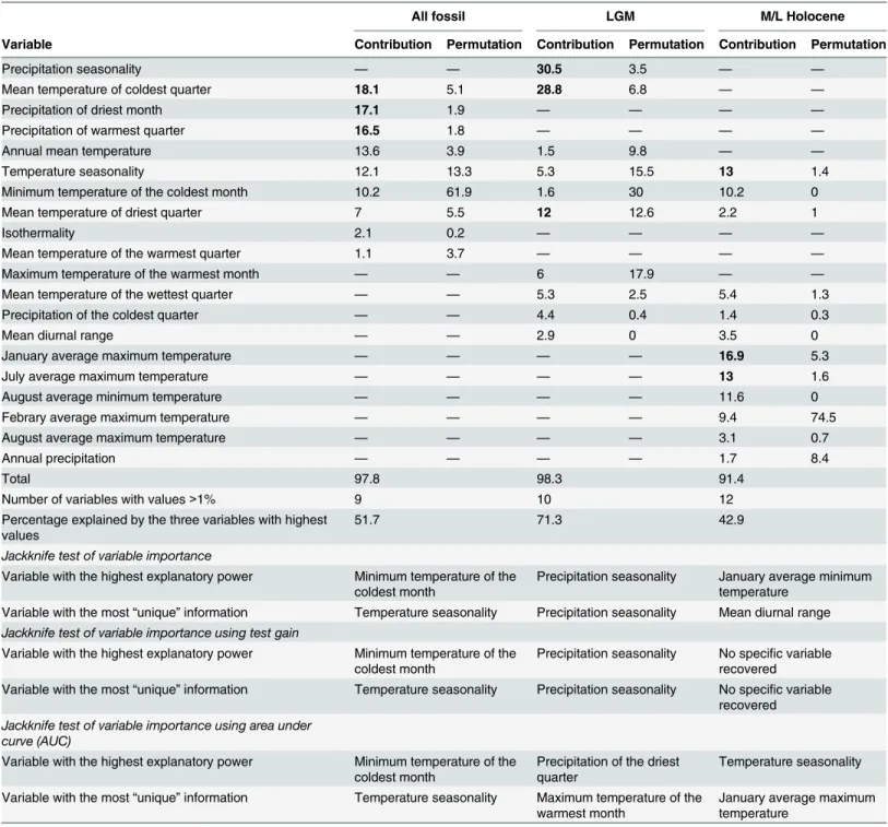
The percent contribution of each variable to the models is presented in
Table 3
for fossil
rec-ords and in
Table 4
for current records. For fossils, eight variables (precipitation seasonality,
mean temperature of the coldest quarter, precipitation of the driest month, precipitation of the
warmest quarter, temperature seasonality, mean temperature of the driest quarter, January
average maximum temperature and July average maximum temperature) contributed
>
40% to
each of the models (
boldface
in
Table 3
). Jackknife tests of variable importance with fossil
rec-ords using training gain, test gain and AUC on test data recovered different sets of variables
(
Table 3
). For current models, four variables (dominant soil, temperature seasonality, August
maximum temperature and precipitation of the warmest quarter) contributed
>
40% to each of
the models (
boldface
in
Table 4
).
The lowest AUC values were found in models with the fewest number of localities for the
species at different times (i.e., LGM and 1950
–
2000). The number of localities used also
influ-enced the prediction values for different areas; fewer records generated maps with coarser
areas, especially in high (0.5
–
1.00) to medium (0.25
–
0.50) prediction values (Figs
2B
and
3C
).
The small number of localities also had an effect on the number of environmental variables
Fig 2. Potential distribution models forLestodelphys halliusing fossil records.A) All-fossil, includes all fossil records from the Pleistocene and Holocene; B) LGM, includes records from the Pleistocene and early Holocene; C) Middle to late Holocene (M/L Holocene), includes fossil records up to ~6000 years before present. Scale bar: 1000 km.
used to generate the models, with fewer records
“
needing
”
more environmental information to
explain the potential distribution of the species. This can be seen in the maps generated from
each model, with the one with the smallest number of records (i.e., LGM) showing an
over-pre-diction of high probability areas throughout the potential distribution (
Fig 2
).
Discussion
The largest number of current localities (
>
90% of 124 localities) found for
Lestodelphys halli
were within the Patagonian steppe [
2
,
5
,
6
], where cool and dry climatic conditions are
domi-nant [
29
,
38
]. The potential distribution models show that the geographic range of
L
.
halli
has
changed from the late Pleistocene to the present day. According to these models we can infer
that there was a decrease in suitable habitat conditions for the species, which could be
mirror-ing changes in environmental conditions. Although we did not test biological variables (such
as biotic interactions and adaptation), which could be influencing the species
’
niche [
39
], we
might expect that the future persistence of this species is threatened, considering the results
found in our analyses and the apparent climatic trend.
Our findings support that the presence of
Lestodelphys halli
from the late Pleistocene to the
middle Holocene in the Pampean region can be related both to precipitation and temperature
variables (e.g., precipitation seasonality, mean temperature of the coldest quarter, precipitation
of the driest month, temperature seasonality). However, the models generated with current
rec-ords show that temperature (e.g., temperature seasonality, August minimum temperature) and
dominant soil had a more important contribution. Precipitation of the warmest quarter and
temperature seasonality are variables very well represented in both fossil and non-fossil
mod-els. Therefore, these variables are the determinants of the distribution of
L
.
halli
, which includes
areas with cold and dry weather and pronounced temperature and precipitation seasonality.
Fig 3. Potential distribution models forLestodelphys halliusing current records.A) All current localities, includes all known records since the species description in 1921; B) 1950, includes records after 1950; C) 1950–2000, includes records between 1950 and 2000. Scale bar: 1000 km.
The presence of
L
.
halli
during the late Pleistocene in Buenos Aires Province was associated
with colder and drier climatic conditions, a hypothesis partially supported by the presence of
other mammals [
23
,
40
] and by different lines of evidence [
15
,
23
,
40
–
43
]. Contrasting with
extinctions in other areas of the Southern Hemisphere [
44
], it seems that extinctions in the
Pampas act from the border toward the center of the distributional range, a phenomenon also
seen in some rodents [
45
]. In this context, populations from northern Mendoza and those
Table 3. Percent of contribution of each variable for the three fossil models (All-fossil, LGM and M/L Holocene) generated forLestodelphys halli. Important variables are indicated in boldface.
All fossil LGM M/L Holocene
Variable Contribution Permutation Contribution Permutation Contribution Permutation
Precipitation seasonality — — 30.5 3.5 — —
Mean temperature of coldest quarter 18.1 5.1 28.8 6.8 — —
Precipitation of driest month 17.1 1.9 — — — —
Precipitation of warmest quarter 16.5 1.8 — — — —
Annual mean temperature 13.6 3.9 1.5 9.8 — —
Temperature seasonality 12.1 13.3 5.3 15.5 13 1.4
Minimum temperature of the coldest month 10.2 61.9 1.6 30 10.2 0
Mean temperature of driest quarter 7 5.5 12 12.6 2.2 1
Isothermality 2.1 0.2 — — — —
Mean temperature of the warmest quarter 1.1 3.7 — — — —
Maximum temperature of the warmest month — — 6 17.9 — —
Mean temperature of the wettest quarter — — 5.3 2.5 5.4 1.3
Precipitation of the coldest quarter — — 4.4 0.4 1.4 0.3
Mean diurnal range — — 2.9 0 3.5 0
January average maximum temperature — — — — 16.9 5.3
July average maximum temperature — — — — 13 1.6
August average minimum temperature — — — — 11.6 0
Febrary average maximum temperature — — — — 9.4 74.5
August average maximum temperature — — — — 3.1 0.7
Annual precipitation — — — — 1.7 8.4
Total 97.8 98.3 91.4
Number of variables with values>1% 9 10 12
Percentage explained by the three variables with highest values
51.7 71.3 42.9
Jackknife test of variable importance
Variable with the highest explanatory power Minimum temperature of the
coldest month Precipitation seasonality January average minimumtemperature Variable with the most“unique”information Temperature seasonality Precipitation seasonality Mean diurnal range Jackknife test of variable importance using test gain
Variable with the highest explanatory power Minimum temperature of the
coldest month Precipitation seasonality No specirecoveredfic variable Variable with the most“unique”information Temperature seasonality Precipitation seasonality No specific variable
recovered Jackknife test of variable importance using area under
curve (AUC)
Variable with the highest explanatory power Minimum temperature of the coldest month
Precipitation of the driest quarter
Temperature seasonality
Variable with the most“unique”information Temperature seasonality Maximum temperature of the
warmest month
January average maximum temperature
Table 4. Percent contribution of each variable for the three current models (All current, 1950 and 1950–2000) generated forLestodelphys halli. Important variables are indicated in boldface.
All current 1950 1950–2000
Variable Contribution Permutation Contribution Permutation Contribution Permutation
Dominant soil 1.8 0.5 23.2 1.5 1.1 0.3
Temperature seasonality 21.6 0.5 15.8 0.3 20.8 0.1
August maximum temperature 14.1 0 — — 12 0
Precipitation of warmest quarter 9.8 0 1 0.7 11.8 2.6
June mean temperature 7.8 0.1 1 0 3 0
July mean temperature 1.1 0.1 — — 5.8 0.2
Febrary maximum temperature 6.2 0.2 — — 5 0.5
December precipitation 5.7 74.9 6.1 54.5 1.9 81.1
January precipitation — — 6.1 0 — —
Mean temperature of wettest quarter 4.6 0.1 3.9 0 3.9 0.1
Mean temperature of coldest quarter 3.9 0.3 4.7 0 3.5 0.2
Isothermality 2.6 0.1 — — 2.8 0.4
January maximum temperature 2 0.1 — — 2.3 0
September mean temperature 1.4 0.1 — — 1.2 0
Mean temperature of driest quarter 1.1 0.4 — — 2.3 0.3
August mean temperature 1.1 0.2 2.5 0 2.4 0.1
June maximum temperature 1 0.1 1.4 0 1.9 0
Maximum temperature of warmest month 1 0 — — — —
July maximum temperature — — — — 4.9 0.1
September minimum tempearature — — 4.2 28 — —
Parental material — — 5.2 0.1 — —
Precipitation seasonality — — 3 1.1 — —
April minimum temperature — — 2.8 2.1 — —
Global vegetation coverage — — 2.7 0.2 — —
Altitude — — 2.6 0.4 — —
June minimum temperature — — 1.8 6.2 — —
Land-form — — 1.2 0.2 — —
August precipitation — — 1.1 0.5 — —
October mean temperature — — 1 0 — —
Total 86.8 77.7 91.3 95.8 86.6 86
Number of variables with values>1% 15 17 17
Percentage explained by the three variables with highest
values 45.5 45.1 44.6
Jackknife test of variable importance
Variable with the highest explanatory power Precipitation of warmest
quarter September minimumtemperature August maximumtemperature
Variable with the most“unique”information Global vegetation coverage Dominant soil Global vegetation coverage Jackknife test of variable importance using test gain
Variable with the highest explanatory power Precipitation of warmest quarter
Dominant soil Precipitation of warmest quarter
Variable with the most“unique”information Land-form Dominant soil No specific variable recovered Jackknife test of variable importance using area under
curve (AUC)
Variable with the highest explanatory power Precipitation of warmest
quarter Isotermality Precipitation of warmestquarter
Variable with the most“unique”information No specific variable
recovered No specirecoveredfic variable No specirecoveredfic variable
scattered in central La Pampa Provinces appear to be more vulnerable to becoming extinct,
because these areas have been experiencing more mesic conditions during the last century [
46
].
A similar result was found by Schiaffini et al. [
47
] for the Patagonian weasel
Lyncodon
patago-nicus
, a species that has often been reported to inhabit environmental conditions similar to
those inhabited by
L
.
halli
, and used as an indicator of cold and dry climatic conditions [
48
].
The absence of
L
.
halli
in central and southern Patagonia during the late Pleistocene-early
Holocene [
18
,
22
,
49
] could also be attributed to physiological constraints. Didelphids are
char-acterized by low basal metabolic rates, high thermal conductance and low body temperatures
[
50
]. Therefore, the climatic conditions of the Late Glacial and Postglacial periods might have
been too extreme for
L
.
halli
[
43
] in southern Patagonia.
During the last 5000 years (middle Holocene to Present), the distribution range of
Lestodel-phys halli
has shown a clear shift, from a distribution concentrated in central and eastern
Argentina, to a southern and western Patagonian distribution (Figs
2
and
3
). The late Holocene
distribution of
L
.
halli
suggests an almost complete disappearance of the species from the
Pam-pean region, consistent with changes along this period towards a more mesic and humid
cli-mate in central Argentina [
15
,
51
]. Only one record in Napostá Grande was recorded in
Buenos Aires Province for the late Holocene [
52
]. In Patagonia, the species has become extinct
from the northeastern area, including several localities in Península Valdes (e.g., Punta Norte,
Ea. San Pablo) and in the lower course of the Chubut River (e.g., Cueva Caolinera, Lle Cul), as
well as the localities of 1 km E Riacho San José, 5 km E Puerto Madryn, Punta Ninfas and
Punta León (
Table 3
). Furthermore, in southern Patagonia the species has disappeared from
the central coast of Santa Cruz Province [
19
].
The models generated with the current localities are consistent with what is known about
the geographic distribution of the species [
2
,
5
]. These models show two large high-prediction
areas in Patagonia, one in western Río Negro and northwestern Chubut Provinces, and another
mostly restricted to northeastern Santa Cruz Province (
Fig 3
). In addition, very restricted
high-to medium-prediction areas were found scattered surrounding the hypothesized relict records
(e.g., those in Mendoza and La Pampa Provinces). Interestingly, despite intensive sampling, no
individuals were trapped or recovered from owl pellets outside what we consider relict areas
(
S1 Fig
). We note that in the 1950 (
Fig 3B
) and 1950
–
2000 (
Fig 3C
) models, prediction values
around the type locality are medium to low. The specimen collected by T. H. Hall, which O.
Thomas used for the original description of
Lestodelphys halli
, was captured around 1920 in
Cape Tres Puntas, on the eastern coast of northern Santa Cruz Province (
Fig 1
). Despite the
low prediction values in this area, the species was found 63 km west of the type locality (record
124;
Table 2
), suggesting that
L
.
halli
is still present near the area where it was collected more
than 90 years ago [
1
,
53
].
Two events have shaped the recent distribution of
Lestodelphys halli
. One event is ancient,
and through it the species has experienced a shift from the Pampas to the Patagonian steppe
and Monte desert. In the other event, during the latest Holocene, the species experienced a
retraction in areas of high (0.5
–
1.00) to medium (0.25
–
0.5) prediction values throughout
Pata-gonia. The latter shows that this opossum is contracting from a broad Patagonian distribution
to core areas in central-northern Patagonia and northern Santa Cruz Province. The models
presented in this work suggest that these changes are mostly driven by climatic variables (i.e.,
precipitation and temperature). These are not minor issues because the regional extinctions of
small mammals are a widespread phenomenon in southern South America [
45
,
54
] and have
involved several sigmodontine and caviomorph rodent species [
22
,
55
–
57
].
end of this century. This will trigger the loss of biodiversity, the extinction of several species, a
decline in water supply, and a decrease in the yields of very important crops, among others
[
59
]. The geographic distribution of
Lestodelphys halli
is mainly modeled by temperature
sea-sonality, August minimum temperature and dominant soil, and this species has lost more than
150,000 km
2in eastern Patagonia during the late Holocene. Considering the findings of our
work and that Patagonia is not exempt from adverse climatic changes, we might expect a harsh
impact on the distribution range of this opossum in the near future.
The information provided in this work highlights the importance of potential distribution
maps as tools to better understand the processes linked to recent regional and local extinctions.
This information also allows adding testable data for the use of some species as proxies for
cli-matic conditions, both in the past and the present. Moreover, understanding the processes that
are behind this kind of phenomenon is essential to elaborate adequate conservation plans.
Supporting Information
S1 Fig. Localities with absence of
Lestodelphys halli
.
Map depicting the absence of
L
.
halli
in
owl pellets with more than 90 individuals per sample.
(TIF)
Acknowledgments
We thank D. Podestá, J. Pardiñas, J. Sanchez, W. Udrizar Sauthier, and M. Carrera for helping
in field and laboratory work. We also thank to the Secretaría de Cultura, Flora y Fauna y
Tur-ismo y Áreas Naturales Protegidas of Chubut Province for work permits, and to the Fundación
Vida Silvestre Argentina (Alejandro Arias, Andrés Johnson, Rafael Lorenzo and Esteban
Bre-mer) for providing facilities and logistical support at the wildlife reserve San Pablo de Valdés.
Finally, are grateful to the anonymous reviewers, F. Prevosti and the Academic Editor P. Wilf,
who helped to improve an earlier version of this manuscript with their helpful comments. This
is contribution number 6 of Grupo de Estudios de Mamíferos Australes (GEMA), Argentina.
Author Contributions
Conceived and designed the experiments: AEF GMM. Performed the experiments: GMM.
Analyzed the data: AEF GMM PT AEC DEUS UFJP. Contributed reagents/materials/analysis
tools: AEF GMM PT DEUS UFJP. Wrote the paper: AEF GMM PT AEC DEUS UFJP.
References
1. Thomas O. A new genus of opossum from southern Patagonia. Annu Mag Nat Hist Ser 9. 1921; 8: 136–139.
2. Martin GM. Sistemática, Distribución y Adaptaciones de Los Marsupiales Patagónicos. PhD. Thesis, Facultad de Ciencias Naturales y Museo Universidad Nacional de La Plata, La Plata, Buenos Aires, Argentina. 2008.
3. Pardiñas UFJ, Teta P, Udrizar Sauthier DE. Mammalia, Didelphimorphia and Rodentia, Southwest of
the Province of Mendoza, Argentina. Check List. 2008; 4: 218–225.
4. Teta P, Pereira J, Fracassi N, Bisceglia S, Heinonen Fortabat S. Micromamíferos del Parque Nacional Lihué Calel, La Pampa, Argentina. Mastozool Neot. 2009; 16: 183–198.
5. Formoso AE, Udrizar Sauthier DE, Teta P, Pardiñas UFJ. Dense-sampling reveals a complex
distribu-tional pattern between the southernmost marsupialsLestodelphysandThylamysin Patagonia, Argen-tina. Mammalia. 2011; 75: 371–379.
6. Birney EC, Monjeau JA, Phillips CJ, Sikes RS, Kim I.Lestodelphys halli: new information on a poorly known Argentine marsupial. Mastozool Neot. 1996; 3: 171–181.
8. Marshall LG. Lestodelphys halli. Mammalian Species. 1977; 81: 1–3.
9. Birney EC, Sikes RS, Monjeau JA, Guthmann N, Phillips CJ. Comments on Patagonian marsupials from Argentina. In: Genoways HH, Baker RJ, editors. Contributions in mammalogy: a memorial volume honoring Dr. J. Knox Jones, Jr. Museum of Texas Tech University, Lubbock, TX; 1996. pp. 149–15. 10. Martin GM. Intraspecific variation inLestodelphys halli(Marsupialia: Didelphimorphia). J Mammal.
2005; 86: 793–802.
11. Udrizar Sauthier DE, Carrera M, Pardiñas UFJ. Mammalia, Marsupialia, Didelphidae,Lestodelphys halli: New records, distribution extension and filling gaps. Check List. 2007; 3: 137–140.
12. Martin GM. Nuevas localidades para marsupiales patagónicos (Didelphimorphia y Microbiotheria) en el noroeste de la provincia de Chubut, Argentina. Mastozool Neot. 2003; 10: 148–153.
13. Formoso AE. Ensambles de micromamíferos y variables ambientales en Patagonia continental extra-andina argentina. PhD. Thesis, Facultad de Ciencias Naturales y Museo, Universidad Nacional de la Plata, La Plata, Buenos Aires, Argentina. 2013.
14. Giarla TC, Jansa SA. The role of physical geography and habitat type in shaping the biogeographical history of a recent radiation of Neotropical marsupials (Thylamys: Didelphidae). J Biogeogr. 2014; 41: 1547–1558.
15. Prado JL, Goin F, Tonni EP.Lestodelhys halli(Mammalia, Didelphidae) in Holocene sediments of Southern Buenos Aires Province (Argentina): morphological and paleoenvironmental considerations. In: Rabassa J, editor. Quaternary of South America and Antarctic Peninsula; 1985. pp. 93–107. 16. Goin FJ. Los Marsupiales. In: Alberdi MA, Leone G, Tonni EP, editors. Evolución biológica y climática
de la Región Pampeana durante los últimos cinco millones de años. Museo Nacional de Ciencias
Nat-urales, Consejo Superior de Investigaciones Científicas, Madrid; 1995. pp. 165–179.
17. Martinelli AG, Forasiepi AM, Jofré GC. El registro deLestodelphysTate, 1934 (Didelphimorphia, Didel-phidae) en el pleistoceno tardío del noreste de la provincia de Buenos Aires, Argentina. Pap Avulsos Zool. 2013; 53: 151–161.
18. De Santis LJM, Tejedor F, Straccia PC. Nuevos registros deLestodelphys halli(Marsupialia: Didelphi-dae). Neotrópica. 1995; 41: 85–85.
19. Zubimendi MA, Bogan S.Lestodelphys hallien la Provincia de Santa Cruz (Argentina). Primer hallazgo en un sitio arqueológico en la costa patagónica. Magallania. 2006; 34: 107–114.
20. Udrizar Sauthier DE. Los micromamíferos y la evolución ambiental durante el Holoceno en el río Chu-but (ChuChu-but, Argentina). PhD. Thesis, Facultad de Ciencias Naturales y Museo Universidad Nacional de La Plata, La Plata, Buenos Aires, Argentina. 2009.
21. Goin FJ. Los Didelphoidea (Mammalia, Marsupialia) del Cenozoico tardío de la Región Pampeana. PhD. Thesis, Facultad de Ciencias Naturales y Museo, Universidad Nacional de La Plata, La Plata, Buenos Aires, Argentina. 1991.
22. Pardiñas UFJ. Los roedores muroideos del Pleistoceno tardío-Holoceno en la región pampeana (sector
este) y Patagonia (República Argentina): aspectos taxonómicos, importancia bioestratigráfica y signifi-cación paleoambiental. PhD. Thesis, Facultad de Ciencias Naturales y Museo, Universidad Nacional de La Plata. 1999.
23. Tonni EP, Cione AL, Figini AJ. Predominance of arid climates indicated by mammals in the pampas of Argentina during the Late Pleistocene and Holocene. Palaeogeogr Palaeoclimatol Palaeoecol. 1999; 147: 257–281.
24. Goin FJ. Marsupiales (Didelphidae: Marmosinae & Didelphinae). In: Mazzanti DI, Quintana CA, editors. Cueva Tixi: Cazadores y recolectores de las Sierras de Tandilia Oriental. Laboratorio de Arqueología, Universidad Nacional de Mar del Plata, Publicación Especial 1, Mar del Plata; 2001. pp. 75–113. 25. Burkart R, Bárbaro NO, Sánchez RO, Gómez AD. Eco-regiones de la Argentina. Programa de
Desar-rollo Institucional, Componente de Política Ambiental, Administración de Parques Nacionales, Buenos Aires, Argentina; 1999.
26. Cabrera AL. Fitogeografía de la República Argentina. Sociedad Argentina de Botánica. 1971; 14: 1–42.
27. Labraga J, Villalba R. Climate in the Monte Desert: Past trends, present conditions, and future projec-tions. J Arid Environ. 2009; 73: 154–163.
28. Cabrera AL, Willink A. Biogeografía de América Latina. Secretaría General de la Organización de los Estados Americanos. Programa Regional de Desarrollo Científico y Tecnológico. Serie de Biología, Monografía N°13. Washington DC; 1973.
30. Ameghino F. Contribución al conocimiento de los mamíferos fósiles de la República Argentina. Actas de la Academia Nacional de Ciencias en Córdoba. 1889; 6: 1–1027.
31. Phillips SJ, Anderson RP, Schapire RE. Maximum entropy modeling of species geographic distribu-tions. Ecol Model. 2006; 190: 231–159.
32. Collins WD, Bitz C, Blackmon ML, Bonan GB, Bretherton CS, et al. The Community Climate System Model: CCSM3. J Climate. 2004; 9: 2122–2143.
33. Gent PR, Danabasoglu G, Donner LJ, Holland MM, et al. The Community Climate System Model Ver-sion 4. J Climate. 2011; 24: 4973–4991.
34. Hijmans RJ, Cameron SE, Parra JL, Jones PG, Jarvis A. Very high resolution interpolated climate sur-faces for global land areas. Int J Climatol. 2005; 25: 1965–1978.
35. Dijkshoorn JA, Huting JRM, Tempel P. Update of the 1:5 million Soil and Terrain Database for Latin America and the Caribbean (SOTERLAC; version 2.0). Report 2005/01, ISRIC—World Soil Informa-tion, Wageningen; 2005.
36. Merow C, Smith MJ, Silander JA. A practical guide to MaxEnt for modeling species’distributions: what it does, and why inputs and settings matter. Ecography. 2013; 36: 1058–1069.
37. Phillips SJ, Dudík M, Schapire RE. A maximum entropy approach to species distribution modeling. Pro-ceedings of the 21stInternational Conference on Machine Learning, Banff, Canada; 2004.
38. León RJC, Bran D, Collantes M, Paruelo JM, Soriano A. Grandes unidades de vegetación de la Pata-gonia extra andina. In: Oesterheld M, Aguiar MR, Paruelo JM, editors. Ecosistemas patagónicos. Eco-logía Austral. 1998; 8: 125–144.
39. Veloz SD, Williams JW, Blois JL, He F, Otto-Bliesner B, Liu Z. No-analog climates and shifting realized niches during the late quaternary: implications for 21st-century predictions by species distribution mod-els. Global Change Biology. 2012; 18:1698–1713.
40. Pardiñas UFJ, Deschamps C. Sigmodontinos (Mammalia, Rodentia) Pleistocénicos del sudoeste de la
Provincia de Buenos Aires (Argentina): Aspectos sistemáticos, paleozoogeográficos y paleoambien-tales. Estudios Geológicos. 1996; 52: 367–379.
41. Pardiñas UFJ. Condiciones áridas durante el Holoceno Temprano en el sudoeste de la Provincia de
Buenos Aires (Argentina): vertebrados y tafonomía. Ameghiniana. 2001; 38: 227–236.
42. Iriondo MH, García NO. Climatic variations in the Argentine plains during the last 18000 years. Palaeo-geogr Palaeoclimatol Palaeoecol. 1993; 101: 209–220.
43. Rabassa J, Coronato A, Martínez O. Late Cenozoic glaciations in Patagonia and Tierra del Fuego: an updated review. Biol J Linn Soc Lond. 2011; 103: 316–335.
44. Woinarski JCZ, Burbidge AA, Harrisond PL. Ongoing unraveling of a continental fauna: Decline and extinction of Australian mammals since European settlement. Proc Natl Acad Sci. 2015; 112: 4531–4540. doi:10.1073/pnas.1417301112PMID:25675493
45. Teta P, Formoso A, Tammone M, de Tommaso DC, Fernández FJ, Torres J, Pardiñas UFJ.
Microma-míferos, cambio climático e impacto antrópico: ¿Cuánto han cambiado las comunidades del sur de América del Sur en los últimos 500 años? Therya. 2014; 5: 7–38.
46. Viglizzo EF, Roberto ZE, Filippin MC, Pordomingo AJ. Climate variability and agroecological change in the Central Pampas of Argentina. Agriculture Ecosystems and Environment. 1995; 55: 7–16. 47. Schiaffini M, Martin GM, Giménez A, Prevosti FJ. Distribution ofLyncodon patagonicus(Carnivora,
Mustelidae): changes from the Last Glacial Maximum to the present. J Mammal. 2013; 94: 339–350.
48. Prevosti FJ, Pardiñas UFJ. Variaciones corológicas deLyncodon patagonicus(Carnivora, Mustelidae) durante el cuaternario. Mastozool Neot. 2001; 8: 21–39.
49. Pearson AK, Pearson OP. La fauna de mamíferos pequeños de Cueva Traful I, Argentina: Pasado y
Presente. Praehistoria. 1993; 1: 73–89.
50. McNab BK. On the ecological significance of Bergmann’s rule. Ecology. 1971; 52: 845–854.
51. Scheifler N, Teta P, Pardiñas UFJ. Small mammals (Didelphimorphia and Rodentia) of the
archaeolog-ical site Calera (Pampean region, Buenos Aires Province, Argentina): taphonomic history and Late Holocene environments. Quatern Int. 2012; 278: 32–44.
52. Deschamps CM, Tonni EP. Los vertebrados del Pleistoceno tardío-Holoceno del Arroyo Napostá Grande, Provincia de Buenos Aires. Aspectos paleoambientales. Ameghiniana. 1992; 29: 201–210. 53. Thomas O. The mammals of Señor Budin’s Patagonian expedition, 1927–28. Annals and Magazine of
Natural History (London), series 10. 1929; 4: 35–45.
54. Pardiñas UFJ, Moreira G, García-Esponda C, de Santis LJM. Deterioro ambiental y micromamíferos
55. Pardiñas UFJ, Udrizar Sauthier DE, Teta P. Micromammal diversity loss in central-eastern Patagonia
over the last 400 years. J Arid Environ. 2012; 85: 71–75.
56. Pardiñas UFJ, Teta P. Holocene stability and recent dramatic changes in micromammalian
communi-ties of northwestern Patagonia. Quatern Int. 2013; 305: 127–140.
57. Teta P, Pardiñas UFJ, Silveira M, Aldazabal V, Eugenio E. Roedores sigmodontinos del sitio
arqueoló-gico“El Divisadero Monte 6”(Holoceno Tardío, Buenos Aires, Argentina): taxonomía y reconstrucción
ambiental. Mastozool Neot. 2013; 20: 171–177.
58. Parry ML, Canziani OF, Palutikof JP, van der Linden PJ, Hanson CE. IPCC 2007. Climate Change 2007: Impacts, Adaptation and Vulnerability. Contribution of Working Group II to the Fourth Assess-ment Report of the IntergovernAssess-mental Panel on Climate Change. Cambridge University Press, Cam-bridge, UK; 2007.
59. Magrin G, Gay García C, Cruz Choque D, Giménez JC, Moreno AR, Nagy GJ, Nobre C, Villamizar A. Latin America. In: Climate Change 2007: Impacts, Adaptation and Vulnerability. Contribution of Work-ing Group II to the Fourth Assessment Report of the Intergovernmental Panel on Climate Change, Parry M.L., Canziani O.F., Palutikof J.P., van der Linden P.J. and Hanson C.E., Eds., Cambridge Uni-versity Press, Cambridge, UK; 2007. pp. 581–615.
60. Odreman R, Zetti J. Addenda paleontológica. In: de Salvo OE, Ceci JH, Dillon A, editors. Caracteres geológicos de los depósitos eólicos del Pleistoceno superior de Junín (Provincia de Buenos Aires). Actas IV Jornadas Geológicas Argentinas, Mendoza, April 6–16. Vol. 1: 269–92. Asociación Argentina de Geología, Buenos Aires; 1969. pp. 291–292.
61. Silveira M. Análisis e interpretación de los restos faunísticos de la Cueva Grande del Arroyo Feo. Rela-ciones de la Sociedad Argentina de Antropología, Nueva Serie. 1979; 13: 229–253.
62. Massoia E. Restos de mamíferos recolectados en el paraje Paso de los Molles, Pilcaniyeu, Río Negro. Revista de Investigaciones Agropecuarias, INTA. 1982; 17: 39–52.
63. Tonni EP, Fidalgo F. Geología y paleontología de los sedimentos del pleistoceno en el area de Punta Hermengo (Miramar, Prov. de Buenos Aires, Rep. Argentina). Aspectos paleoclimáticos. Ameghiniana. 1982; 19: 79–108.
64. Perrota EJB, Pereda I. Nuevos datos sobre el alero IV del Tromen (Dto. Picunches, Prov. de Neuquén). In: Comunicaciones de las Primeras Jornadas de Arqueología de la Patagonia. Editado por Dirección de Cultura de la Provincia del Chubut, Rawson, Chubut; 1987. pp. 249–258.
65. Reig OA, Kirsch JAW, Marshall LG. Systematic relationships of the living and Neocenozoic "opossum-like" marsupials (suborder Didelphimorpha), with comments on the classification of these and of the Cretaceous and Paleogene New World and European metatherians. In: Archer M, editor. Possums and Opossums, Studies in Evolution. Chipping Norton, Surrey Beaty y Sons Pty and Royal Zoological Soci-ety of New South Wales; 1987. pp. 1–89.
66. Oliva F, Gil A, Roa M. Recientes investigaciones arqueológicas en el sitio San Martín 1 (BU/PU/5), Par-tido de Puán, Provincia de Buenos Aires. Shincal 3, Actas del Congreso Nacional de Arqueología Argentina. Catamarca; 1991. pp. 135–139.
67. Neme G, Moreira G, Atencio A, de Santis L. El registro de microvertebrados del sitio arqueológico Arroyo Malo 3 (Provincia de Mendoza, Argentina). Rev Chil Hist Nat. 2002; 75: 409–421. 68. Andrade A, Teta P. Micromamíferos (Rodentia y Didelphimorphia) del Holoceno Tardío del sitio
arqueológico alero Santo Rosario (provincia de Río Negro, Argentina). Atekna. 2003; 1: 274–287.
69. Horovitz I. Restos faunísticos de La Martita y nuevo registro biogeográfico deLestodelphys hally (Didel-phidae, Mammalia). In: Aguerre AM, editor. Arqueología y paleoambiente en la Patagonia Santacru-ceña Argentina; 2003. pp. 87–91.
70. Pardiñas UFJ. Roedores sigmodontinos (Mammalia: Rodentia: Cricetidae) y otros micromamíferos
como indicadores de ambientes hacia el Ensenadense cuspidal en el sudeste de la provincia de Bue-nos Aires (Argentina). Ameghiniana. 2004; 41: 437–450.
71. Teta P, Andrade A, Pardiñas UFJ. Micromamíferos (Didelphimorphia y Rodentia) y paleoambientes del
Holoceno tardío en la Patagonia noroccidental extra-andina (Argentina). Archaeofauna: 2005; 14: 183–197.
72. Deschamps CM. Late Cenozoic mammal bio-chronostratigraphy in southwestern Buenos Aires Prov-ince, Argentina. Ameghiniana. 2005; 42: 733–750.
73. Simpson GG. Didelphidae from the Chapadmalal Formation in the Museo Municipal de Ciencias Natur-ales of Mar del Plata. Museo Municipal de Ciencias NaturNatur-ales, Mar del Plata. 1972; 2: 1–39.
74. Reig O. El segundo ejemplar conocido deLestodelphys halli(Thomas) Mammalia, Didelphydae). Neo-trópica. 1959; 5: 57–58.
76. Pearson O. Mice and the postglacial history of the Traful Valley of Argentina. J Mammal. 1987; 68: 469–478.
77. Massoia E, Pardiñas UFJ. Presas de Bubo virginianus en Cañadón Las Coloradas, Departamento
Pilca-niyeu, Río Negro. Boletín Científico, Asociación para la Protección de la Naturaleza. 1988; 4: 14–19. 78. Massoia E, Pardiñas UFJ. Pequeños mamíferos depredados porBubo virginianusen Pampa de
Nes-tares, Departamento Pilcaniyeu, Provincia de Río Negro. Boletín Científico, Asociación para la Protec-ción de la Naturaleza. 1988; 3: 23–27.
79. Pardiñas UFJ, Massoia E. Roedores y marsupiales de Cerro Castillo, Paso Flores, Departamento
Pil-caniyeu, provincia de Río Negro. Boletín Científico, Asociación para la Protección de la Naturaleza. 1989; 13: 9–13.
80. Massoia E, Pastore H. Análisis de regurgitados deBubo virginianus magellanicus(Lesson, 1828) del Parque Nacional Laguna Blanca, Dpto. Zapala, Pcia. de Neuquén. Boletín Científico, Asociación para la Protección de la Naturaleza. 1997; 33: 18–19.
81. Pardiñas UFJ, Galliari CA. La distribución del ratón topoNotiomys edwardsii(Mammalia: Muridae). Neotrópica. 1998; 44: 123–124.
82. Andrade A, Teta P, Panti C. Oferta de presas y composición de la dieta deTyto alba(Aves: Tytonidae) en el sudoeste de la provincia de Río Negro, Argentina. Historia Natural (Segunda Serie). 2002; 1: 9–15.
83. Teta P, Andrade A. Micromamíferos depredados porTyto alba(Aves: Tytonidae) en las Sierras de Talagapa (provincia del Chubut, Argentina). Neotrópica. 2002; 48: 88–90.
84. Pardiñas UFJ, Teta P, Cirignoli S, Podestá DH. Micromamíferos (Didelphimorphia y Rodentia) de
nor-patagonia extra andina, Argentina: taxonomía alfa y biogeografía. Mastozool Neot. 2003; 10: 69–113. 85. Gasco A, Rosi MI, Durán V. Análisis arqueofaunístico de micro-vertebrados en“Caverna de las Brujas”
(Malargüe-Mendoza-Argentina). Anales de Arqueología y Etnología, Volumen especial. 2006, 61: 135–162.
86. Nabte MJ, Saba SL, Pardiñas UFJ. Dieta del Búho Magallánico (Bubo magellanicus) en el desierto del
monte y la Patagonia Argentina. Ornitol Neotrop. 2006; 17: 27–38.
87. Rodríguez VA, Theiler GR. Micromamíferos de la región de Comodoro Rivadavia (Chubut, Argentina). Mastozool Neot. 2007; 14: 97–100.
88. Schiaffini M, Giménez A, Martin GM. Didelphimorphia and Rodentia (Mammalia) from Sierras de Tecka and surrounding areas, northwestern Chubut, Argentina. Check List. 2011; 7: 704–707.