Novembro de 2015
Working
Paper
407
Fiscal policy in Brazil: from
counter-cyclical response to crisis
TEXTO PARA DISCUSSÃO 407•NOVEMBRO DE 2015• 1
Os artigos dos Textos para Discussão da Escola de Economia de São Paulo da Fundação Getulio
Vargas são de inteira responsabilidade dos autores e não refletem necessariamente a opinião da
FGV-EESP. É permitida a reprodução total ou parcial dos artigos, desde que creditada a fonte.
Escola de Economia de São Paulo da Fundação Getulio Vargas FGV-EESP
1
Fiscal policy in Brazil:
from counter-cyclical response to crisis
Márcio Holland
São Paulo School of Economics at Getulio Vargas Foundation, Brazil1
This version: November 10th
, 2015
Abstract
The main goal of this article is to identify the dynamic effects of fiscal policy on output in Brazil
from 1997 to 2014, and, more specifically, to estimate those effects when the output falls below its
potential level. To do so, we estimate VAR (vector autoregressive) models to generate
impulse-response functions and causality/endogeneity tests. Our most remarkable results indicate the
following channel of economic policy in Brazil: to foster output, government spending increases
causing increases in both tax rates and revenue and the short-term interest rate. A fiscal stimulus via
spending seems efficient for economic performance as well as monetary policy; however, the latter
operates pro-cyclically in the way we defined here, while the former is predominantly countercyclical.
As the monetary shock had a negative effect on GDP growth and GDP growth responded positively
to the fiscal shock, it seems that the economic policy has given poise to growth with one hand and
taken it with the other one. The monetary policy is only reacting to the fiscal stimuli. We were not
able to find any statistically significant response of the output to tax changes, but vice versa seems
work in the Brazilian case.
1
Corresponding author: [email protected]. This working paper was partially written during my mandatory cooling-off period when I spent part of this time as a visiting scholar at Columbia University in the City of New York and for this reason I am very grateful to Professors Albert Fishow, Thomas Trebat, Gray Newman, Sidney Nakahodo, Gustavo
Azenha, and Daniella Diniz, for having me and giving me all support I needed to develop my research. However, all
2
1. Introduction
The 2008 international financial crisis put fiscal policy at the forefront of debate, particularly
its use in mitigate the painful effects of the crisis on outputs and employment. Probably because of the
lack of widely recognized rules, fiscal policy is generally a controversial issue. The economic
meltdown with its deep and protracted impact on both goods and labor markets presented the perfect
opportunity to approach divergent views about its use. For a few years after the 2008 crash, there was
no room for austerity until government debts skyrocketed. Alas, governments had to shift towards
fiscal retrenchment, even under economic weakness. The results of recent fiscal policy have been
mixed, and its effectiveness remains a disputed issue.
On the other hand, a stream of literature has conducted empirical studies with novel
methodologies in an effort to identify the dynamic and contemporaneous effects of fiscal policy on
outputs. Auerbach and Gorodnichenko (2012) estimate a government purchase multiplier for a large
number of OECD countries using a specific form of the STVAR (smooth transition vector
autoregressive) model and have identified a fiscal multiplier in both recession and expansion
circumstances. The model might be considered a refinement of Blanchard and Perotti’s (2002)
specification, who used a simplified structural VAR model. In 2014, Mineshima et al. introduced a
TVAR (threshold vector autoregressive) model to use when regimes are determined by a transition
variable, which is either exogenous or endogenous. More recently, Herwartz and Lütkepohl (2014)
proposed a structural vector autoregression model with Markov switching that combines conventional
and statistical identification of shocks, which can be useful for future studies on fiscal policy.
The main goal of this article is to identify the effect of fiscal shocks on the output in Brazil
from 1997 to 2014, and, more specifically, to estimate those effects when the output falls below its
potential level, as observed during most of the period following the 2008 international meltdown. We
pose an additional question: How low can the output drop when it is already below its potential level
(which we call “negative initial conditions” for the fiscal consolidation program), despite the
composition of the fiscal retrenchment? In other words, after the output has bottomed out, how can
policymakers quickly instill confidence by cutting expenditures and increasing taxes when these
measures were supposed to be implemented an expansionary shock?
To do so, we estimate VAR (vector autoregressive) models to generate impulse-response
functions and causality tests. Our most remarkable results indicate the following channel of economic
policy in Brazil: to foster output, government spending increases, causing increases in both tax rates
and revenue and the short-term interest rate. A fiscal stimulus via spending seems quite efficient for
3
the former is predominantly countercyclical. We were not able to find any statistically significant
response of the output to tax changes, but we did find a statistically significant response of tax changes
to the output in the Brazilian case.
The contributions of this work are threefold: first, it identifies the response of the output to
fiscal and monetary policy; second, it estimates the impact of recent fiscal measures on the output;
and, third, in line with broader economic literature, it suggests a long-term fiscal plan for Brazil to
spur its effectiveness in reducing output losses.
This work is divided in the following sections. The next section shows Brazil’s recent
experience with fiscal policy and its main results. The third section presents the literature and
discussions of the effectiveness of fiscal policy. The fourth section extrapolates the impulse-response
functions obtained in our research to measure the potential impact of the 2015 fiscal plan on output
and confidence. Ultimately, it is the appropriate moment to present the advantages and caveats of our
empirical procedures. We are most aware of the many drawbacks presented in this sort of time series
analysis. At the end of this section, we suggest a long-term fiscal plan for Brazil using lessons learned
from both Brazil’s recent experience with fiscal policy and our empirical study.
2. The Brazilian Context
Governments across the globe responded to the 2008 crisis with unprecedented expansionary
actions in recent economic history. Monetary and fiscal countercyclical actions were implemented to
both stymie the contamination of the international crisis in financial systems and to resume growth as
soon as possible.
From 2008 to 2010, fiscal and monetary stimuli were overwhelmingly recommended.
However, since 2010, the focus has shifted to fiscal consolidation in advanced economies. Since then,
fiscal results have improved over the world, even though the debt-to-GDP ratios remain high
compared with those before the crisis. More recently, the United States has outperformed the euro
area, where calling for austerity appears to have fallen out of fashion again, as illustrated in the 2015
Greek case.
The fiscal front has deteriorated dramatically in many advanced economies with mixed and far
from outstanding achievements. However, comparing the 1929 Great Depression with the 2008 Great
4
response, unemployment in the United States peaked at 10 percent in 2010. Though this was still
disturbingly high, it was far below the catastrophic 25 percent scaled in the Great Depression”.
Due to this thought, the Brazilian government took a series of countercyclical policies to
protect the local economy from crumbling. These policies seemed to work well, at least until 2013.
The worst of the crisis was absorbed without any major disruption in the Brazilian economic system.
Most importantly, the economy resumed growth in the 2nd
quarter of 2009; the unemployment rate
did not spike; real wages continued to grow; and consumer and business confidence recovered very
quickly. Nevertheless, after a period of recovery until 2013, the overall growth remained
disappointing, particularly given the very rapid deterioration in 2014, the expected strong contraction
in 2015, and uncertainty about 2016 performance.
From late 2014 to early 2015, Brazil launched a tight fiscal program. The pro-cyclical biased
fiscal consolidation plan is presumably considered the only plausible policy stance when solvency
became the issue rather than economic activity. In Brazil, the diagnosis and prescription have been far
from divergent. However, as highlighted by Frankel (2012), “a pro-cyclical fiscal policy magnifies the
severity of the business cycle”. This controversy motivated this research to assess whether such fiscal
consolidation policies are expected to hurt GDP growth to a greater extend because the economy is
already under contraction. Alternatively, would they spur confidence so that the drag on economic
activity could be avoided?
There is no doubt that fiscal stimuli were needed at that challenging time, when the Brazilian
economy was severely hit by the financial crisis. As for fiscal policy, there were considerable tax
exemptions in 2009. As a result of the actions taken by the government at that time, the country was
able to recover very quickly from the crisis; among other things, Brazil experienced 7.6 percent and
3.9 percent growth in 2010 and 2011, respectively (see table 1).
According to the national account’s new dataset, released on March 27, 2015 by the National
Bureau of Statistics (IBGE), the 2008 crises hit the economy harder and deeper, and the recovery was
faster and better because investment resumed quickly and included a greater share of the GDP
compared with the previous period of the crisis, regardless of its volatility (see figure 1 and 2).
In early 2011, the Federal Administration was able to start applying a fiscal consolidation plan
to cool down the economy. Needless to say, solvency had not been a problem in Brazil for a long
time, as international reserves have been considerable and more than enough to pay for external
liabilities; in addition, the public debt-to-GDP ratio had been decreasing over the years. Thanks to
5
which could be considered incredibly low in comparison with the debt dynamics in advanced
economies after the crisis. However, the general gross debt-to-GDP ratio is still high in Brazil
compared with that of its peers, although it had been relatively stable, even during most of the period
of countercyclical fiscal policy (see table 1 and figures 2 and 3 for the fiscal results).
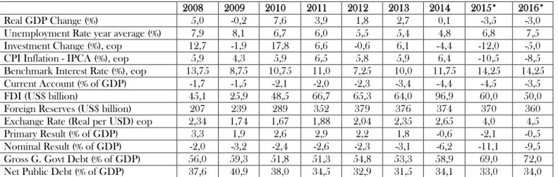
Table 1. Brazil: Key Macroeconomic Indicators after the 2008 Crisis (2008-2015)
2008 2009 2010 2011 2012 2013 2014 2015* 2016*
Real GDP Change (%) 5,0 -0,2 7,6 3,9 1,8 2,7 0,1 -3,5 -3,0
Unemployment Rate year average (%) 7,9 8,1 6,7 6,0 5,5 5,4 4,8 6,8 7,5
Investment Change (%), eop 12,7 -1,9 17,8 6,6 -0,6 6,1 -4,4 -12,0 -5,0
CPI Inflation - IPCA (%), eop 5,9 4,3 5,9 6,5 5,8 5,9 6,4 -10,5 -8,5
Benchmark Interest Rate (%), eop 13,75 8,75 10,75 11,0 7,25 10,0 11,75 14,25 14,25
Current Account (% of GDP) -1,7 -1,5 -2,1 -2,0 -2,3 -3,4 -4,4 -4,5 -3,5
FDI (US$ billion) 45,1 25,9 48,5 66,7 65,3 64,0 96,9 60,0 50,0
Foreign Reserves (US$ billion) 207 239 289 352 379 376 374 370 360
Exchange Rate (Real per USD) eop 2,34 1,74 1,67 1,88 2,04 2,35 2,65 4,0 4,5
Primary Result (% of GDP) 3,3 1,9 2,6 2,9 2,2 1,8 -0,6 -2,1 -0,5
Nominal Result (% of GDP) -2,0 -3,2 -2,4 -2,6 -2,3 -3,1 -6,2 -11,1 -9,5
Gross G. Govt Debt (% of GDP) 56,0 59,3 51,8 51,3 54,8 53,3 58,9 69,0 72,0
Net Public Debt (% of GDP) 37,6 40,9 38,0 34,5 32,9 31,5 34,1 33,0 34,0
Notes: Unemployment rate is yearly average of the Monthly Employment Survey (PME); CPI is the broad CPI (IPCA); Benchmark interest rate is the target Central Bank interest rate in the end of period; and exchange rate as in the end of period. eop = end of period. * 2015 and 2016 are author´s forecasts.
Source: Ministry of Finance of Brazil, Central Bank of Brazil, and IBGE.
Even with such policies, the primary surplus targets were fully accomplished, at least until
20122
(see figure 2). However, by mid-2012 to 2013, the recovery appeared to be weaker than
expected, and the Brazilian economic authorities returned to incentives, trying to reignite the
economy3
. In 2013, the economy grew again by 2.7%, and the investment grew 6.1%. A wide tax relief
program and increasing government expenditures, including a broad financial subsidy for credit for
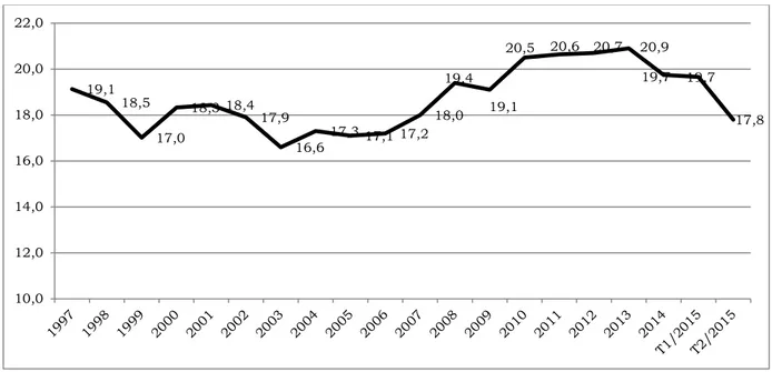
capital goods via public banks, were introduced. The economy reacted reasonably, so the investment
to GDP ratio remained relatively stable at approximately 20.5% until at least 2013, despite its high
variability (see figure 1).
2
Although the one-off revenues had increased in importance after the 2008 crash, responding, for instance, to 0.74% and 0.85% of GDP in 2009 and 2010, respectively, when the full primary surplus delivered was 1.9% and 2.6% of GDP, respectively, or, in 2013, when 0.68% of 1.8% of GDP was one-off revenue. In 2014, one-off revenue was 0.5% of GDP while the primary deficit was 0.6% of GDP. 2015 primary surplus is going to be plenty of on-off revenue, as well.
3
6
Figure 1. Brazil: Gross Formation of Fixed Capital as % of GDP) 1997-2015
Source: IBGE, updated in November 17, 2015.
Note: Investment as % of GDP measured using current values for GDP and gross formation of fixed capital. 2015 is author´s forecast.
Figure 2: Nominal Fiscal and Primary Results as Share of GDP (%) 1999-2018
Source: Central Bank of Brazil; 2015 - 2018 are author´s forecast.
However, from 2013 to 2014, the output was not responding at all to tax stimuli or even
spending increases. After Brazil graduated to respond to the 2008 crisis using countercyclical fiscal
policies (Vègh and Vulletin, 2013), it experienced a rapid deterioration on the fiscal front in 2014.
Both net and gross public debt increased quickly towards a risky case scenario, so the investment 19,1
18,5
17,0
18,3 18,4 17,9
16,6 17,3 17,1 17,2 18,0
19,4
19,1
20,5 20,6 20,7 20,9
19,7 19,7
17,8
10,0 12,0 14,0 16,0 18,0 20,0 22,0
(5,20)
(3,30) (3,30) (4,40)
(5,20) (2,90)
(3,50) (3,60) (2,70) (2,00)
(3,20) (2,40) (2,50) (2,30) (3,10) (6,20)
(11,10) (9,50)
(7,40) (6,00) 2,80 3,20 3,30 3,20 3,20
3,70 3,70
3,20 3,20 3,30
1,90 2,60 2,90 2,20 1,80
(0,60) (2,10)
(0,50)
0,50 1,00
(12,00) (10,00) (8,00) (6,00) (4,00) (2,00) 2,00 4,00 6,00
1999 2000 2001 2002 2003 2004 2005 2006 2007 2008 2009 2010 2011 2012 2013 2014 2015 2016 2017 2018
7
grade rating was no longer assured in the medium term4
. Potential output decreased at the same time
as the output was well below its declining potential output level.
In late 2014 and early 2015, some social benefits were reviewed, and some tax relief was
reverted (tables 5.1 and 5.2 detail these measures). The economy had actually started to adjust itself
during 2014, as the Central Bank had begun a new tightening cycle from April 2013 to July 2014. The
target interest rate increased 375 basis points in an interval of one year. Another 325 basis-point
increase would take place between October 2014 and July 2015. A 700 basis-point monetary shock in
an interval of two years is far from negligible. Its primary side effect was a considerable contraction in
the domestic credit on durable and capital goods, contributing to an additional drop in consumer and
business confidence.
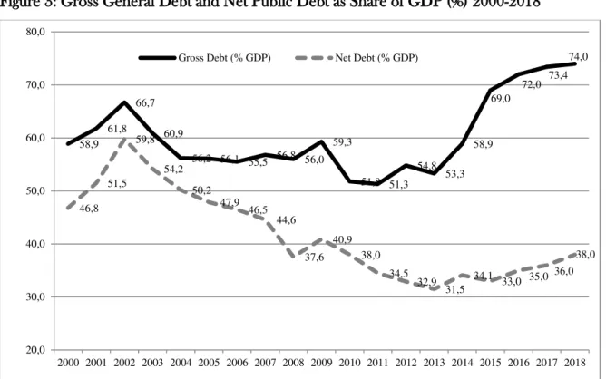
Figure 3: Gross General Debt and Net Public Debt as Share of GDP (%) 2000-2018
Source: Central Bank of Brazil; 2015-2018 are author´s forecasts.
Since mid-2014 the Brazilian economy fell into full disarray: a combination of fiscal crisis with
strong and prolonged GDP contraction in the midst of a political chaos. There are many plausible
explanations for the deceleration of the economic, including the monetary policy shock, associated
curbing in household credit for durable goods, and the gradual increase in some tax rates. Meanwhile,
the economy suffered from a myriad of other events, such as long-standing and severe drought,
corruption scandals involving the largest Brazilian state-run oil company and major entrepreneurs in
4 September 2015, a couple of weeks after the Government had decided to send to Congress the 2016 Budget Law with
deficit, the Standard & Poor´s downgraded the Brazilian sovereign rating to speculative grade.
58,9 61,8
66,7 60,9
56,2 56,1 55,5 56,8 56,0 59,3
51,8 51,3 54,8
53,3 58,9
69,0
72,0 73,4 74,0
46,8 51,5
59,8 54,2
50,2 47,9
46,5 44,6
37,6 40,9
38,0 34,5
32,9
31,5 34,1 33,0 35,0 36,0
38,0
20,0 30,0 40,0 50,0 60,0 70,0 80,0
8
the civil construction sector, low government popularity amid street protests and general disapproval
regarding the corruption scandals, several bribery schemes, and the 2014 FIFA World Cup. There
are also drivers associated with a profounder phenomenon, as many analysts believe that the previous
consumption-based growth model had already been exhausted. Unfavorable terms of trade are also
remembered as another key driver of such exhaustion.However, I would highlight the exhaustion of
domestic economic cycle as the main guilty for such difficulties, which could dramatize the GDP
performance in coming years. Under this circumstance, the economy became very sensitive to either
domestic or external shocks.
Therefore, fiscal results had been worsening faster than predicted, as the tax revenue had been
frustrated in line with the growth downturn. Gross debt, as a percentage of the GDP, increased from
53.3% in December 2013 to 58.9% in December 2014 and, then, soar to 66%, September 2015. The
gross debt prospects indicate further increases towards over 70% of GDP by the end of 2016 (see
figure 3). In addition, surprisingly, the nominal deficit increased from 3.1 to 6.2% of GDP and
skyrocketed to 9.34% of GDP in September 2015, a movement that was driven by interest payments,
which also increased to 8.9% of GDP. Debt maturity and denomination have deteriorated with the
same intensity.
As risks are tilted towards deep GDP contraction in 2015 and also in 2016, fiscal sustainability
appears to have been an important issue yet again. For instance, in September 2015, the net revenues
of the central government decelerated -4.6% year-to-dates comparing to 2014. In that month, the
government spending also declined -4.0%, in the same terms, although less than the tax frustration.
Consequently, the rolling 12-month primary surplus of the central government decreased to -0.5% of
GDP in September 2015. However, the primary surplus is expected to be delivered will be even
worse and can reach 2.1% of GDP. Tax revenue frustration is only partial explanation. In 2015, the
government could not take into account the relevant amount of one-off revenues; and also it had to
pay the delayed expenses, domestically labeled as “fiscal pedaling”.
Brazil fell into a severe fiscal crisis: the country failures to reach the required primary
surpluses, that is, the level necessary to stabilize debt to GDP, this year and even in coming years.
Therefore, the gross debt to GDP ratio is expected to soar 72% of GDP in 2016, from 53% of GDP,
in 2013. This crisis is predicted to last many years. As far as I can tell, there is no solution, not even a
light at the end of the tunnel.
The causes of such a fiscal situation are closely related to the causes of the GDP contraction.
First, I would consider the stronger-than-expected GDP contraction that leads to tax revenue
9
related to income transfer programs such as pension benefits5
, LOAS6
, Minha Casa Minha Vida
(housing program), Bolsa-Família (a conditional cash transfer program), etc. I would also include the
reluctance in implementing the appropriate fiscal consolidation plan of early 2015. This hesitancy
amplified the uncertainty on the economic recovery. Finally, because of the second round of the
counter-cyclical fiscal policy implemented in 2012, delayed expenditures had to be settled during
2015. Meanwhile, intense realignment in the regulated price provoked a high short-term inflation. It
seems there are many plausible explanations for such a drama experienced by the Brazilian economy
like a perfect storm.
From a long-term perspective, as seen in figure 4, there has been a considerable change in
government spending since 2003, as it has been focused on reducing income inequality via increasing
conditional cash transfer programs. The federal budget for education and housing has been increasing
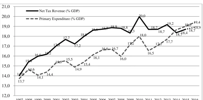
over the years. Total federal expenditures increased from 14.6% of GDP in 1997 to 18.6% of GDP at
the end of 2014. Meanwhile, the net total federal tax revenue increased from 15.4% to 19.9% of GDP
in 2010 and then decreased to 18.4% at the end of 2014. The recent fiscal stimuli combined to
increase government expenditures by almost 1% of GDP, while the tax revenue declined from 19.8%
to 18.4% of GDP. However, such recent efforts did not ignite growth in 2014. Many analysts question
whether the overall fiscal multipliers decreased over this period of time. If so, why?
Figure 4. Brazil: Net Tax Revenue and Government Spending (% of GDP)1997-2016
Source: IBGE, and Ministry of Finance, Brazil. 2015 forecast according to the Minister of Planning.
5 The deficit in the general pension system is expected to reach 2.0% of GDP in 2016 from 1.0% of GDP in 2014. 6 LOAS is a welfare public policy for elderly with the benefits indexed to minimum wage. Its expenditure reached 0.7%
of GDP, in 2014.
14,0 15,4
16,0 16,2 17,0
17,7 17,2
18,0
18,6 18,7 18,9 18,8 18,3 20,0
18,7 18,7
19,2
18,4 18,7 18,9
13,7 14,6
14,1 14,4
15,3 15,5 14,9
15,4 16,1
16,6 16,7 16,0
17,2 18,0
16,5
17,1 17,7 18,7
19,0 19,4
12,0 13,0 14,0 15,0 16,0 17,0 18,0 19,0 20,0 21,0
1997 1998 1999 2000 2001 2002 2003 2004 2005 2006 2007 2008 2009 2010 2011 2012 2013 2014 2015 2016 Net Tax Revenue (% GDP)
10
So, what happened with the government expenditure over time? What are the main
components of such increases? First of all, according to the table 2, the primary spending increased
2.8% of GDP since 2002, which is practically the same growth level of income transfers to
households. Pension benefits show the most relevant increase followed by a welfare benefit for the
elderly called LOAS. Part of the growth is related to both generous eligibility criteria and also public
policy stance, due to the fact that the benefits are indexed to the minimum wage corrections.
As a matter of curiosity, because of this indexation rule, the benefits increased 78%, in real
terms, in the last 10 years. At the same time, the number of beneficiaries increased by 9 million
people, from 23 million to 32 million. Meanwhile, the government decided to enlarge social
programs such as Bolsa Família and Minha Casa Minha Vida. Both are responsible for a 0.63% of
GDP variation in the government consumption during this period of time.
Table 2. The Main Government Expenditure (2002-2014) % of GDP and Percentage Point (pp)
2002
(% GDP)
2010 (% GDP)
2014 (% GDP)
Variation 2002-2014 pp
Variation 2011-2014 pp
PRIMARY SPENDINGS 15,58 16,91 18,35 2,77 1,43
Payroll 4,77 4,28 3,98 -0,79 -0,30
Income Transfer to Households 6,51 8,25 9,31 2,79 1,05
Pension Benefits 5,90 6,56 7,14 1,24 0,58
Unemployment Insurance and Wage Bonus 0,48 0,77 0,98 0,49 0,21
Welfare Benefits (LOAS/RMV) 0,00 0,58 0,70 0,70 0,12
Bolsa-Família (income transfer to poor) 0,13 0,35 0,49 0,36 0,14
Investments 0,82 1,17 1,30 0,48 0,13
Fixed Gross Capital Formation 0,82 1,15 1,04 0,21 -0,11
Minha Casa Minha Vida (housing program) 0,00 0,02 0,27 0,27 0,25
Expenditures 3,48 3,21 3,76 0,28 0,55
Health 1,38 1,34 1,42 0,04 0,07
Education 0,43 0,55 0,76 0,33 0,21
Subsidies* 0,16 0,21 0,16 0,01 -0,04
Others 1,51 1,11 1,41 -0,09 0,31
Net Revenue minus Income Tranfer 11,18 9,87 8,73 -2,46 -1,14
Source: National Treasure and IBGE. Author´s calculation.
Note: * Subsides herein is taking into consideration only those due to the correspondent years. Implicit and explicit subsides, that is, the financial and credit subsides, started to be estimated only in 2012; since then they are 0.9% do GDP in annual average, according to the methodology developed by the Secretariat of Economic Policy at the Minister of Finance.
Moreover, there appears to be an increase of the financial and credit subsides related to the
funding provided by the National Treasure to the state-owned banks. According to the table 2, the
subsidies have been stable over time. However, this measurement doesn´t take into account the
implicit and explicit subsidies, in particular those with delayed payments. Roughly speaking, as part of
11
enterprises offering low interest rates and the National Treasure was committed to equalize the
interest rates. For instance, the BNDES provided subsidized long-term credit for investments in
machineries and in the infrastructure sector. The difference between the benchmark rate Selic and
the long-term interest rate called TJLP defines the size of the subsidy offered by the BNDES. The
larger the difference between the two rates, the larger the subsidy. According to the calculations
conducted by the Secretariat of Economic Policy, those subsidies reached an annual average of 0.9%
of GDP in 2012-2014, much higher than the data provided in the table 2.
Therefore, more beneficiaries, sizable correction in the benefits and enlarged income transfer
programs could be considered the most relevant factors to explain the augmented expenditures. At
the same time, tax revenues remained relatively stable until 2013. Since 2014 a drop was enough to
make vulnerable the annual fiscal results; yet fiscal expansions were no longer financed by tax
revenue.
The situation became even worse because the deficit in the pension system soared surprisingly
fast. After a certain period of stability, the deficit is projected to double from 2014 to 2016, from 1%
to 2% of GDP. Pension system is responsible for 40% of the total expenditure followed by “payroll”
with 20%. Its expenditures are foreseen to increase more than $25 billion in a very short interval of
time, from 2014 to 2016. Figure 5 shows this risky scenario. As can be fairly seen, the spending has
increased faster than the revenue. The slow increase in the revenue is because of the weakness of the
labor market, which means the higher the unemployment rate, the lower the labor formalization and
then the lower the pension revenues. The spending increase, as mentioned before, is due to the
generous benefit criteria of eligibility, and an upsurge in the minimum wage, which indexes the
benefits.
The demography dynamics in Brazil is also a challenging task for the pension system, since
the population is ageing quickly. This issue is likely to be the major explanation for the growth in the
pension system deficit in the coming years. A comprehensive reform in the system is required. It
would embrace much more strict criteria for newcomers such as minimum eligible age, similar
treatment for gender, de-indexation of benefits from minimum wage, revision of some special
12
Figure 5. Pension System in Brazil: revenue, spending and deficit (% of GDP) 2005-2016
Source: National Congress.
3. The Literature and Our Case Study
The discussion on the effectiveness of fiscal policy is mostly associated with the fiscal
multiplier, either for government purchases or tax revenue. However, the literature indicates that
there is no unique fiscal multiplier. Furthermore, there is scarce literature about emerging market
economies and no theoretical support for whether multipliers should be expected to be higher or
lower than in the advanced economies (Estevão and Samake, 2013; Ilzetzki et al., 2013; Ilzetzki,
2011; IMF, 2008; and Kraay, 2012). Some studies even conclude that multipliers are negative,
particularly in the longer term (IMF, 2008) and when public debt is high (Ghosh and Rahman, 2008).
One can easily find very divergent fiscal multipliers (see table 2). The multiplier depends on
the critical factors, such as trade openness, the exchange rate regime, the fiscal instrument (whether
spending or tax-based), the debt level, the monetary policy stance (whether normal or
zero-lower-bound), and the state of the economy (whether contracting or expanding). Despite such innumerable
factors, the fiscal multiplier is also sensitive to the method of estimation. For instance, the DSGE
approach has shown larger multiplier than the VAR approach. However, as highlighted by
Mineshima et al. (2014:319), the DSGE model presents difficulties in modeling nonlinearity and does
so differently compared with the Taylor rule for monetary policy, as “there is no widely accepted
fiscal policy (rule) to be included in a DSGE model”.
108 124 140
163 182 212
246
276 307
338 350 366
146 166
185 200 225
255 281
317
357
394
427
491
1,73 1,75
1,65
1,17
1,29
1,10
0,81
0,87
0,97 1,03
1,32
2,00
0,50 1,00 1,50 2,00 2,50
100 200 300 400 500 600
2005 2006 2007 2008 2009 2010 2011 2012 2013 2014 2015 2016
13
Table 2. Fiscal Multipliers Survey: the GDP growth response to fiscal shocks
Authors Country/ Region
Methodology Sample GDP growth response to one SD +/-2S.E innovation on government spending
Blanchard and Perotti (2002)
United States SVAR 1947.1 to 1997.4
Peak values from 0.97 to 1.29 4-quarter response: 0.45 to 0.55 Christiano et al.
(2009)
United States DSGE From 0.8 (no zero bound) to 3.4 (under zero bound)
Auerbach and Gorodnichenko (2012)
OECD countries
STVAR
1960.1-2010.4
From 0.6 (under expansion) to 2.5 (under recession)
Alesina et al. (2014)
17 OECD countries
Quasi-panel based on a truncated MA representation
1978-2009
From close to 0.0 (if spending-based plan) to -3.0 (if tax-based plan) both after 4-quarter response
Meneshima et al. (2014)
OECD and G7
Countries
TVAR 1970.1 to
2010.4
From 0.72 (positive output gap) to 1.22 (negative output gap) after 4-quarter response
On the other hand, VAR models are subject to several critics. Commodity-exporting
countries, such as Brazil, may experience revenue changes because of booms and busts in the
international commodities market, not because of discretionary fiscal policy. As VAR models suffer
from the omitted variable problem and required quarterly data might not be available for a long
enough time span, they can limit identifying information. In the specific case of the Brazil, the longest
possible time span results in 72 observations over the course of 18 years, including the last years of a
pegged exchange-rate regime (1997-1998). According to Ilzetzki (2011), the more fixed the exchange
rate regime, the larger the fiscal multiplier. Therefore, our results may be biased when we use the full
sample (1997-2014).
Brazil is considered a closed economy, and this attribute is expected to increase the fiscal
multiplier. As Brazilian trade openness does not present relevant changes over time, we do not expect
that any sort of influence of such a key variable on the identification of the multiplier using
country-specific VAR models. Although trade openness is highly recommended for many other reasons, if the
policymakers are really interested in using a discretionary fiscal policy to obtain any real output effect,
the current closed economy makes their fiscal efforts more effective. However, if the effectiveness of
the fiscal policy is falls short of policymakers’ expectations, trade policy should be implemented to
achieve a more economic opening.
Many efforts have been made to show the importance of the fiscal instruments. As widely
14
and the fiscal multiplier of the former is likely higher than that of the latter. Moreover, the procedure
of Alesina et al. (2014) involves a simulation of a multi-year fiscal plan rather than of individual fiscal
shocks. According to the authors’ findings, “Fiscal adjustments based upon spending cuts are much
less costly, in terms of output losses, than tax-based ones and have especially low output costs when
they consist of permanent rather than stop and go changes in taxes and spending”. As the authors
explain, “The difference between tax-based and spending-based adjustments appears not to be
explained by accompanying policies, including monetary policy. It is mainly due to the different
response of business confidence and private investment”.
Our case study has no multi-year fiscal plan and no fiscal policy adjustment based only on
spending cuts. The only goal is to reach the annual announced primary surplus, regardless of the
instrument and composition. Late 2014, 1.2% of GDP expressed in terms of the amount of money
(e.g., $22 billion) is due as public sector consolidated primary surplus by end of 2015, and there was
also a target of 2.0% of GDP for the coming years. It was hard to identify the proportion of spending
cuts and tax hikes needed to obtain such surpluses. However, the fiscal measures announced (see
table 5.1 and 5.2) defined approximately 2.2% of GDP7
in overall savings through spending cuts
(approximately 1.75% of GDP) and increased taxes (approximately 0.54% of GDP).
Alas, these measures did not directly assure a movement from a deficit of 0.6% of GDP, in
December 2014, to a surplus of 1.2% of GDP in December 2015. Actually, another primary deficit is
expected in 2015 and, moreover, surplus for next year is not guaranteed. The government most likely
will deliver a deficit of at least 1.1% of GDP, instead of a surplus of 1.2% of GDP announced last
December 2014. It is a dramatically poorer scenario. But, why such an unpleasant surprise? First,
most of the savings come from the 2015 federal budget cut, which is generally overestimated; second,
the increase in tax rates does not imply the same increase in tax revenue, which is more related to
economic performance8
; and, finally, the revision in some social benefits takes time to contribute to
fiscal efforts. Moreover, alongside the extreme deterioration of the domestic economic activity
pushing down the tax revenue, payments of delayed expenditures have worsened the fiscal balance.
Austerity brings more contraction, and such a circumstance is tough to obtain tax revenue. The back
and forth economic policy stance during the year also played its role for such drama. It had to include
low extraordinary revenue that put a negative bias to the fiscal balance.
7 This value is overestimated as it includes cut in an inflated budget. Taking into account only the structural spending
cuts, the plan would retrench only 0.26% of GDP.
8
15
Our case study is more associated with shifts in fiscal policy over time than with long-term
fiscal consolidation programs. The VAR model can capture this short-term dynamic adjustment,
although Brazil instead have a fiscal plan that is well designed and communicated for the coming
years. In line with Alesina et al. (2014), this sort of plan could result in a shorter recession than would
be expected in our case study, as experienced recently.
The debt level is very important, especially with the debt threshold is below the international
threshold, as in the Brazilian case. According to the economic literature, the lower the debt threshold,
the smaller the fiscal multiplier. In Ilzetzki (2011), the fiscal multiplier can eventually become negative
when the debt exceeds its threshold. Brazil obtained sound results in terms of net debt levels until at
least 2013; the gross debt-to-GDP ratio is higher than those of its peers, and debt maturity has
remained a concern. The implicit interest rate of the debt is much higher than the monetary policy
rate, which is considered one of the most persistently highest in the world. Because of this debt
constraint, Brazil is expected to show a small fiscal multiplier. In other words, fiscal stimuli are
welcome during contractions, without losing sight of debt sustainability in the medium term.
The state of the economy is one critical factor of the fiscal multiplier. Using regime-switching
models, Auerbach and Gorodnichenko (2013) estimated the effects of fiscal policies that might vary
over the business cycle. They found considerable differences in the size of spending multipliers
during recessions and expansions, with fiscal policy being considerably more effective in recessions
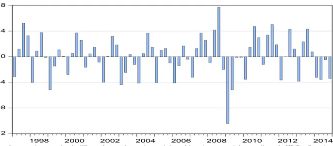
than in expansions. As can be seen in the figure 6, Brazil’s output is running well below its potential
level, as roughly measured by the HP filter, throughout 2014, and it will most likely be the same
throughout 2015 and 2016. In this scenario, the fiscal multiplier is expected to be larger than the
previous years. Puzzlingly, fiscal stimuli recently seem to not being working well at all.
As is well known, the effectiveness of fiscal policy is heterogeneous under normal
circumstances (Favero, Giavazzi, and Perego, 2011). In the case of conventional monetary policy,
fiscal laxity may have a restricted impact on output. Otherwise, countercyclical fiscal policy is likely to
smooth the business cycle. The debt level is a constraint in both cases but is most likely a major issue
for developing economies. In line with the Easterly’s (2013) idea, part of the public debt increase is
considered “normal” in advanced economies. However, in the aftermath of the 2008 turmoil,
conventional monetary policy has been used mostly in developing economies, where debt intolerance
(Reinhart et al., 2003) is still considered a relevant phenomenon.
A simplified debt sustainability assessment unveils such a relevant constraint for the coming
years and the peril of a downgrade in the sovereign rating. Under a baseline scenario, gross general
16
to stabilize debt are higher than that formerly targets announced by Brazilian policymakers for 2015
and 2016; however, it is quite difficult to reach even that 1.2% of GDP target for 2015 and the 2% of
GDP target for 2016. A bleak slowdown does not allow tax revenue to increase, even with the tax
benefit withdrawals announced9
early 2015.
In sum, an upward bias for the fiscal multiplier is expected, which is associated with a couple
of years under the pegged exchange-rate regime (1997-1998) and with the contractions during the
2008 financial turmoil and since at least the middle of 2013. There has been a downward bias for the
fiscal multiplier caused by the debt level and the accompanying conventional monetary policy stance.
There is also the recessionary bias of the recently announced fiscal measures (in late 2014 and early
2015).
Figure 6. Brazil Output Gap - % Quarterly Data (1997-2014)
Note: Output gap is measured as the difference between the actual output in log and the estimate output in log according to the HP filter (Lampda = 1,600).
3. The Empirical Model and Findings
We roughly estimate the basic VAR model. The specification considers aggregate government
purchases in the linear model with no regime shifts or control for expectations, including the
following ordering [G T Y i] for Cholesky decomposition:
(1) � = � �, � �−1+ �
where � ≡ [ �, ��, � is a three-dimensional vector in the logarithms of quarterly taxes, spending,
benchmark interest rate, and GDP, all in real terms. �≡ [��, ��, ��]′ is the corresponding vector of
reduced-form residuals, which generally have nonzero cross correlations.
9
17
We then expand our estimations to take into account confidence indicators and disaggregate
variables. In � ≡ [ �, ��, �], Xt is an n-dimensional vector, including business and consumer
confidence, private investment and household consumption10
, besides interest rate and real GDP.
We are aware that VAR models have been subject to several criticisms (IMF, 2010; Romer,
2011; and Caldara and Kamps, 2012). DSGE models are alternative approaches, but they also have
drawbacks. We are also aware that other key macroeconomic variables could be taken into
consideration, such as trade openness, debt level, and financial market deepening. However, the
changes over time used in our estimations are negligible. We would highly recommend including
them in case of a panel-based empirical analysis, as those variables most likely change across
countries.
We adopted the VAR Granger causality/block exogeneity Wald tests to examine the causal
relationships among the variables. Under this system, an endogenous variable can be treated as
exogenous. We used the chi-square (Wald) statistics to test the joint significance of each of the other
lagged endogenous variables in each equation of the model and also for the joint significance of all
other lagged endogenous variables in each equation of the model. The chi-square test statistics for
some variables (X, for example) represent the hypothesis that the lagged coefficients of that variable in
the regression equation of another variable (Y, for example) are equal to or different from zero. If
equal to zero, that variable (X) is Granger causal for Y at some level of significance, which suggests
that Y is not influenced by X. The null hypothesis of block exogeneity is then rejected for all
equations in the model.
The first group of empirical results is related to a very simplified VAR model and its pairwise
Granger causality and block exogeneity Wald tests. Information criteria from Akaike, Hannan-Quinn
and Schwarz were used to select the most parsimonious, correct model. Most tables and figures
presenting the results appear in the Annex. We have conveniently separated some figures to show
alongside the text.
We estimated two different VAR models as follows:
(1) VAR 2: [Y, S, T, i]
10 These results are not reported herein, as they did not add any relevant analysis, but the results are available upon
18
where Y is the GDP; S is the government expenditure as a percentage of GDP deflated by IPCA; T is
the net tax revenue as a percentage of GDP deflated by IPCA; and
i
is the Selic interest rate in annualpercentage terms.
(2) VAR 1: [h, FI, i]
where h is the output gap measure, i.e., the difference between the actual GDP and the potential
GDP according to the HP filter; FI is the fiscal impulse measure, i.e., the variation of the primary
surpluses as a share of GDP; and
i
is the variation of Selic interest rate in annual percentage terms.The VAR model in specification (2) allows us to simultaneously identify the direction of fiscal
and monetary policy. As we split up the sample to cope with the 2008 crash, it is also possible to
observe the eventual shift in the economic policy stance before and after the crisis.
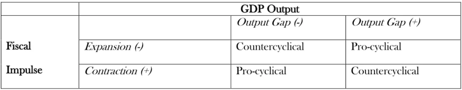
Then, this second specification is more related to the policy stance, whether countercyclical or
pro-cyclical. For instance, fiscal policy could be labeled as countercyclical or pro-cyclical when the
sign of the fiscal impulse is equal to or different from (expansionary or contractionary, respectively)
the signal of the deviation of the real output from its tendency level (the output gap). Figure 7
illustrates this idea. According to this figure, one can have, for example, countercyclical policy under
fiscal adjustments and pro-cyclical stances during output expansion. It is always a matter of the
direction of the fiscal policy alongside the business cycle.
Figure 7. Fiscal Expansion and Contraction
GDP Output
Fiscal
Impulse
Output Gap (-) Output Gap (+)
Expansion (-) Countercyclical Pro-cyclical
Contraction (+) Pro-cyclical Countercyclical
There have been many discussions about countercyclical versus pro-cyclical fiscal policies and
when and how much uses each type. However, the first challenge involves assessing how much of
effort the policymakers intend to make. The most accurate way to infer this effort is by assessing
structural fiscal results instead of conventional ones11
. Before moving on, it is important to consider
that the structural fiscal results are still behind the times when the topic is fiscal rules, mainly because
they are well known only quarters or even years after the fiscal practice is implemented, as they
11
19
depend on many complex calculations. However, if the purpose is to define the intensity of the fiscal
policy, they are more appropriate, even though the other methods are not necessarily incorrect.
The structural fiscal results can be briefly defined as results that are consistent with the
potential output, under the condition of equilibrium in the asset and commodity prices and free of
one-off revenues. It may be considered an accurate form to express the fiscal discretionary effect on
the aggregate demand. As fiscal results can be influenced by many factors beyond the control of
economic authorities, structurally based results consider only the effective fiscal efforts of
policymakers. Conventional results, such as primary surpluses, are not capable of measuring such
efforts because they depend on others factors, such as the business cycle, and, in turn, changes in
asset and commodity prices, changes in output composition, and one-off revenues.
Figure 8 illustrates the use of one-off revenues in Brazil, which increased dramatically after the
2008 crisis. One-off revenues includes: concessions revenue in most years, judicial deposit (in 2009),
Eletrobras’ dividend (in 2009 and 2010), Petrobras capitalization (most of 2010 one-off revenue),
Sovereign Fund of Brazil (created in 2008 and used in 2012), tax refining program (in 2009, 2011,
2013, and 2014), other one-off revenues, dividends in advance, and FND subsidize. The annual
average of one-off revenue from 2009 to 2014 (after the crisis) was 0.6% of GDP when the average of
the annual primary surpluses was 1.8% of GDP, representing, then, 1/3 of the annual fiscal results.
How much policymakers intend to pledge or cut in terms of stimulus or retrenchment,
respectively, during a certain period of time, depends on the fiscal impulse, that is, the difference
between the current structural fiscal result and the previous result. Fiscal policy could be labeled as
countercyclical or pro-cyclical when the signal of the fiscal impulse is equal to or different from
(expansionary or contractionary, respectively) the signal of the deviation of the real output from its
tendency level (the output gap).
Figure 8: One-Off Revenue, 2002-2014 (US$ Billion and % of GDP)
Source: Secretariat of Economic Policy, Minister of Finance of Brazil. Notes: We use 3.0 Brazilian Real per one US Dollar.
-4000,0 -2000,0 0,0 2000,0 4000,0 6000,0 8000,0 10000,0 12000,0 14000,0
2002 2003 2004 2005 2006 2007 2008 2009 2010 2011 2012 2013 2014
0,74
0,02 0,06 0,04 0,04 0,08
-0,23 0,74
0,85
0,38 0,53
0,68 0,50
-0,20 0,00 0,20 0,40 0,60 0,80 1,00
2002 2003 2004 2005 2006 2007 2008 2009 2010 2011 2012 2013 2014
20
Here, the idea is different for the case of monetary policy. It could be pro-cyclical or
countercyclical when the signal of the monetary policy shock (changes in the interest rate) is equal to
or different from (contractionary or expansionary, respectively) the output gap. Then, for instance, we
label arbitrarily a pro-cyclical monetary policy when the interest rate increases during an expansion.
Otherwise, it would be a countercyclical orientation.
We also conducted a multivariate pairwise Granger causality test/block exogeneity Wald test
derived from the VAR model to examine additional causal relationships between the key variables in
the model. This test estimates the χ square value of the coefficients of lagged endogenous variables.
The null hypothesis in this test is that the lagged endogenous variables do not Granger cause the
dependent variable.
Data Descriptions
The models are estimated over three samples: first, the full sample spanning from 1997 to
2014 and then two other samples to determine the eventual effect of the 2008 crash: one from 1997
to 2007 and one from 2008 to 2014. We are aware that the small size of the sample of times series
diminishes the degrees of freedom and the robustness of the estimates.
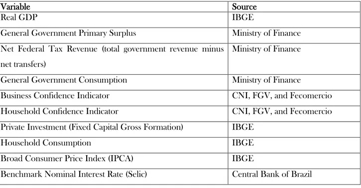
Table 3 shows data descriptions and the sources used here. All series, if necessary, are
deflated with the Broad Consumer Price Index (IPCA) and divided by GDP.
According to our sample, the GDP has grown an average of 0.73% in quarter-over-quarter
terms, which is approximately 3.0% in annualized terms; investment has grown a little faster at 3.2%;
and consumption is coupled with the GDP growth (table 4). There are different speeds over time
because investment has grown faster and consumption has resumed faster than the GDP after the
2008 turmoil. The average investment as share of GDP is 18.7%, with some increases after the crisis
coming to approximately 20%, which could introduce an intriguing question. Net tax revenue as share
of GDP has been higher than the government spending-to-GDP ratio. The volatility of the investment
rates, as measured by standard deviation (approximately 14% in annualized terms), is quite
21
Table 3. Data descriptions and sources
Variable Source
Real GDP IBGE
General Government Primary Surplus Ministry of Finance
Net Federal Tax Revenue (total government revenue minus
net transfers)
Ministry of Finance
General Government Consumption Ministry of Finance
Business Confidence Indicator CNI, FGV, and Fecomercio
Household Confidence Indicator CNI, FGV, and Fecomercio
Private Investment (Fixed Capital Gross Formation) IBGE
Household Consumption IBGE
Broad Consumer Price Index (IPCA) IBGE
Benchmark Nominal Interest Rate (Selic) Central Bank of Brazil
Table 4. Basic Statistics for 1997-2014 (N=72, QoQ Change)
GDP Growth
(%)
Investment Growth
(%)
Consumption Growth
(%)
Investment (%GDP)
Tax Revenue (%GDP)
Governement Spending
(%GDP)
Minimum -4.09 -10.0 -3.0 18.4 13.4 13.7
Maximum 2.76 8.5 2.98 21.6 24.7 20.9
Mean 0.73 0.79 0,72 18.7 17.7 16.03
Standard Deviation
1.17 3.3 1,14 1.45 1.8 1.47
Empirical Findings
Our models were generally run with four lags, according to the information criteria12
. We
estimate a model for the full sample (1997-2014) and for the period before (1997-2007) and after
(2008-2014) the crash13
. We first present results of the impulse-response functions and then the VAR
Granger causality tests/block exogeneity Wald tests, from the VAR 1 specification and then from the
VAR 2 specification. The figures and tables presenting these results appear in the Annex.
First, generally speaking, it is remarkable that the fiscal stimulus via government spending has
a positive and statistically significant impact on GDP growth and that the monetary policy has a
12
The following information criteria are used here: LR = sequential modified LR test statistic (each test at the 5% level); FPE = final prediction error, AIC = Akaike information criterion; SC = Schwarz information criterion; and HQ = Hannan-Quinn information criterion.
13
22
negative and statistically significant impact on GDP growth, regardless of the model and specification.
It is also worth mentioning the channels through which these findings work in the model. On the one
hand, unexpected shocks in government expenditures generally spark growth; on the other hand, they
lead to positive shocks in the short-term interest rate that hinder growth. Additionally, there is no
statistically significant response from any other key macroeconomic variable, including GDP growth
and the confidence related to unexpected shocks in net tax revenue. However, tax revenue responded
slightly positively to shocks in government expenditures and growth. There are mixed results
associated with the relationship among our other key variables, such as government expenditures, net
tax revenues, the fiscal impulse and the short-term interest rate.
More specifically, we first examine the impact of the unexpected structural shock of taxes on
other key variables. According to the VAR Granger causality/block exogeneity Wald test, we cannot
reject the null hypothesis that net tax revenue does not Granger cause GDP growth, but we can reject
the hypothesis that it does not cause government expenditures. GDP growth Granger causes tax
revenue only when we use the full sample and with less statistical significance when we use the
bub-samples from after/before the crash.
According to the impulse-response functions, the response of GDP growth to unexpected
shocks in tax revenue is small and not statistically significant; the size of the response and its
significance is reasonable only when we take the short-term interest rate out of the VAR specification.
In line with the Granger causality test, the response of government spending to a tax shock is positive
and statistically significant.
Therefore, we can summarize the role played by tax policy as follows: increased government
spending increases tax revenue, and the greater the GDP growth, the greater the tax revenue. It seems
that tax revenue has increased because the government has chosen to stimulate the economy using its
spending power.
Now, we turn to the effect of the structural shock of government expenditures. According to
the Granger causality test, one can reject the hypothesis that government spending does not Granger
cause GDP growth, regardless of the sample and the specification.
On the other hand, government spending Granger causes the benchmark interest rate.
Therefore, fiscal policy seems to be very efficient in reviving growth in Brazil, even though it comes
23
In terms of dynamic effects, the GDP growth responds positively, although not necessarily
different from zero, to unexpected shocks in government expenditures, reaching its peak after four
quarters; its peak changes with the sample; using the full sample, the peak is 0.5, but the peak doubles
to 1.1 in the period after the 2008 crash; it is approximating 0.4 for the sample before the crash. It
seems that fiscal policy is even more effective during difficult times. In sum, the size of such impact,
which is generally associated with the fiscal multiplier, is approximately 0.5 after 4 quarters for normal
times and approximately 1.1 after four quarters in difficult times, including the aftermath of the 2008
financial crisis14
.
Meanwhile, GDP growth responds negatively and statistically significantly to the unexpected
shock in the benchmark interest rate. Surprisingly, the response is close to 1.1 for the sample after the
crisis and 0.5 for the full sample and the sample before the crisis. There is no difference between the
monetary and fiscal shocks in terms of the dynamics over time because both affect the GDP after four
quarters.
As the monetary shock had a negative effect on GDP growth and GDP growth responded
positively to the fiscal shock, it seems that the economic policy “has given poise to growth with one
hand and taken it with the other one”.
For instance, some authors have conducted studies on the impact of the rock-bottom interest
rate policy in the US. According to a general New Keynesian model, as explored in Christiano,
Eichenbaum and Rebelo (2010), the government spending fiscal multiplier can be larger than usual
thanks to the monetary policy stance. They analyzed a special case of the zero-lower-bound interest
rate policy in the US and concluded that this policy amplifies the impact of expansionary stimuli.
According to these authors, “First, when the central bank follows a Taylor rule, the value of
the government-spending multiplier is generally less than one. Second, the multiplier is much larger if
the nominal interest rate does not respond to the rise in government spending. For example, suppose
that government spending goes up for 12 quarters and the nominal interest rate remains constant. In
this case the impact multiplier is roughly 1.6 and has a peak value of about 2.3. Third, the value of the
multiplier depends critically on how much government spending occurs in the period during which
the nominal interest rate is constant…for government spending to be a powerful weapon in combating
output losses associated with the zero-bound state” (p. 5-6).
14We, herein, are not intentionally using such coefficients as the well-known fiscal multiplier because of drawbacks in the
24
Does the monetary policy amplify the fiscal policy in the Brazil case? The answer is “no”. The
monetary policy rate has been diminishing over time but has been reacting to the fiscal policy. It is a
sort of “give-and-take policy”, as the persistently high short-term interest rate (see figure 9) under a
conventional Taylor rule-based action considerably reduces the government spending fiscal
multiplier. We also use the actual US federal funds rate to run a VAR that hypothetically assumes a
zero-lower-bound monetary policy in Brazil. In such a hypothetical situation, the response of GDP
growth to unexpected shocks in government expenditures would almost double, from 0.5 to 1.0 using
the full sample and from 1.1 to 1.8 using sample after the 2008 crash, both under the dramatic
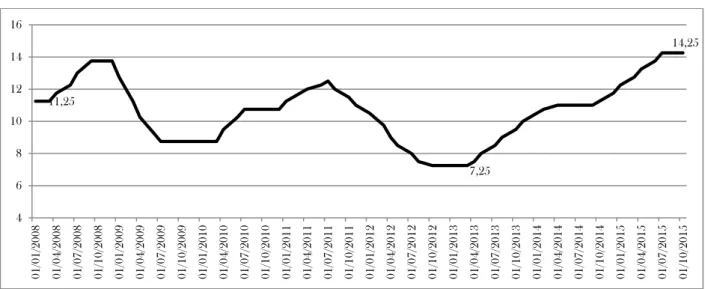
assumption of a zero-lower-bound interest rate in Brazil. Figure 9 shows this story. For instance, the
short-term interest rate increased from 2009 to 2012, and, after a lax cycle, another tight policy stance
arose in 2013. While fiscal policy was predominantly operating in a countercyclical direction,
monetary policy was operating in a pro-cyclical direction.
Figure 9: Benchmark Nominal Interest Rate (2008-2015), annual %
Source: Central Bank of Brazil
Now, we use the VAR 2 [h, F, i] specification to analyze the direction, i.e., countercyclical or
pro-cyclical, of economic policy. The VAR was run with four lags following the information criteria.
At first glance, as seen in figure 11, fiscal policy has been predominantly countercyclical, and
monetary policy has been predominantly pro-cyclical15
. An unexpected shock in the fiscal impulse
(the change in the primary surplus-to-GDP ratio) has a positive and statistically significant impact on
the output gap (the difference between the actual GDP and its potential level). One can clearly see
that the government increases its fiscal results when the economy is doing better and reduces them
under contractions. According to the impulse-response function, the fiscal impulse responds
positively and statistically significantly to the unexpected shock of GDP growth, and vice versa,
15Again, we arbitrarily labeled “pro-cyclical” monetary policy when the interest rate follows the business cycle in the
same direction. This case could fairly be denominated as a counter-cyclical fiscal policy.
25
reaching a peak of 1.2 after three quarters and remaining relatively stable afterwards. Using the
sub-sample after the 2008 crash, this peak jumps up to 1.9, which clearly shows the important role played
by fiscal stimuli during hard times.
Figure 10. Impulse-Response Function VAR [Y, S, T, i]
Meanwhile, unexpected shocks in monetary policy have a negative and statistically significant
impact on the output gap. Monetary policy in Brazil seems more effective than expected. In a
dynamic analysis, the output gap slump in response to the unexpected monetary shock, bottoming out
at -0.5 after two quarters, then increases to -1.7 after five quarter, remaining relatively stable
afterwards. During tough times, using the sub-sample from 2008 to 2014, this peak elevates to 2.0.
The main lesson that we can take from these empirical findings is that monetary shocks have been
large enough to counterweigh any fiscal stimulus over time.
It is worth mentioning that monetary policy has reacted to fiscal policy because the benchmark
interest rate responds negatively to unexpected shocks in the primary surplus. We were not able to
accept the responses of the interest rate set by the Central Bank to shocks nor to net tax revenue nor
to government spending, but we can now observe the importance of primary surpluses to the Central
26
increase in the primary surplus as share of GDP triggers a 30 basis-point decreases in the short-term
interest rate after two quarters.
Figure 11. Impulse-Response Function VAR [h, F, i]
We also include indicators of confidence in variations of both of our VAR specifications16
. As
there would be a causal relationship running from the indicators of business and consumer
confidences to output and investment, we inquired about whether confidence might be resumed
before investment and output. According to Alesina et al. (2014), “the confidence of investors also
does not decrease much after an expenditure-based adjustment and promptly recovers and increases
above the baseline; it instead falls for several years after a tax-based adjustment”.
As leading indicators, indicators of business and consumer confidences could be able to
foresee prospects of output and investment for the coming years. However, the results when we run
specifications that include such variables do not change our previous findings. Confidence indicators,
both for businesses and consumers, respond less than GDP growth to shocks in government
expenditures, net tax revenues, and fiscal impulses. It seems that when the scenario for growth comes
to entrepreneurs’and consumers’ minds, the economy has already found a path to growth.
16