Essays on trade and innovation

(1)

FUNDAÇÃO GETULIO VARGAS ESCOLA DE ECONOMIA DE SÃO PAULO

SYNTHIA KARINY SILVA DE SANTANA

ESSAYS ON TRADE AND INNOVATION

(2)

FUNDAÇÃO GETULIO VARGAS ESCOLA DE ECONOMIA DE SÃO PAULO

ESSAYS ON TRADE AND INNOVATION

Tese apresentada ao Programa de Pós-Graduação da Escola de Economia de São Paulo da Fundação Getulio Vargas, como requisito à obtenção do título de Doutor em Economia.

Orientador: Emanuel Augusto Rodrigues Ornelas.

(3)

Santana, Synthia Kariny Silva de.

Essays on trade and innovation / Synthia Kariny Silva de Santana. - 2016. 87 f.

Orientador: Emanuel Augusto Rodrigues Ornelas Tese (doutorado) - Escola de Economia de São Paulo.

1. FINEP. 2. Exportação. 3. Inovações tecnológicas. 4. Indústria de

transformação. I. Ornelas, Emanuel Augusto Rodrigues. II. Tese (doutorado) - Escola de Economia de São Paulo. III. Título.

(4)

ESSAYS ON TRADE AND INNOVATION

Tese apresentada à Escola de Economia de São Paulo da Fundação Getulio Vargas, como requisito para obtenção do título de Doutor em Economia. Data de aprovação: 29 de julho de 2016.

Banca Examinadora:

Prof. Dr. Emanuel Augusto Rodrigues Ornelas (Escola de Economia de São Paulo)

Prof. Dr. João Paulo Cordeiro de Noronha Pessoa (Escola de Economia de São Paulo)

Prof. Dr. Lucas Pedreira do Couto Ferraz (Escola de Economia de São Paulo)

Prof. Dr. Paulo Furquim de Azevedo (INSPER)

(5)

(6)

AGRADECIMENTOS

“Verba volant, scripta manent”. Por isto gostaria de registrar minha gratidão àqueles que contribuíram direta ou indiretamente para a conclusão do doutorado. Em primeiro lugar, gostaria de agradecer a Deus por ter derramado tantas bênçãos em minha vida.

Agradeço aos meus pais, em meio a tantas renúncias e sacríﬁcios, por terem me proporcionado a oportunidade de perseguir meus objetivos proﬁssionais. Às minhas irmãs Suzany e Sylvia pelo carinho e paciência. À minha família, meu porto seguro.

Aos docentes da Fundação Getulio Vargas pela disposição em compartilhar conhecimento. Ao coordenador Enlinson Mattos cujo apoio institucional foi fundamental assim como o do professor Pedro Valls. Ao professor Paulo Furquim e Verônica Orellano, pela conﬁança, suporte, compreensão e palavras de incentivo. Ao orientador Emanuel Ornelas, por ter me adotado e proporcionado esta oportunidade ímpar. Aos membros da banca de defesa de tese pelas valiosas sugestões. Aos funcionários da FGV/SP por proporcionarem um ambiente agradável de estudos e aprendizado.

Aos amigos da EESP, em especial aos companheiros da “Salinha da Paulista” e aos colegas de Doutorado pelos momentos de cumplicidade e apoio mútuo; aos amigos de graduação e mestrado da UFPE e aos ex-companheiros do programa PET por me encorajarem sempre; aos professores da UFPE Andrea Sales, Alexandre Rands, Francisco Ramos e Jocildo Bezerra por terem me guiado academicamente desde o começo.

Ao IBGE, em especial à GEATE, pelo apoio institucional para a elaboração da tese. Particularmente, meu agradecimento ao Luis Carlos Pinto e ao Carlos Lessa pela paciência e por terem feito tudo o que estava ao alcance para que meus resultados fossem liberados a tempo. Ao Leandro e Glaucia minha profunda gratidão pela ajuda com a base de dados, suas nuances e especiﬁcidades. Agradeço também aos companheiros de sala de sigilo no biênio 2015-2016, cujas idéias e experiências foram essenciais para confecção dos artigos. Aos amigos do Arena Maracanã Hostel, minha segunda família no último ano do doutorado, agradeço pela hospitalidade e companhia de funcionários e colegas de quarto.

Agradeço à CAPES pelo suporte ﬁnanceiro.

Finalmente, à “tia Zezita” e Mirian por me acolherem nesses quatro anos na cidade de São Paulo.

(7)

ABSTRACT

The wide availability of data at the firm level in the past twenty years has opened a new range of opportunities for testing important economic theories. In this thesis we aim to explore the complementarity between international trade and investments on innovation in the Brazilian manufacturing industry. In this framework we recognize that innovation is important for firms both because of the positive externalities that it exhibits as with regard to the social returns it provides. For this reason, governments often subsidize these investments, especially the riskiest ones. However, it is still poorly understood how subsidized firms perform over time as we make clear in the first chapter. Although the Economic Subvention Program (ESP) operated by FINEP has aimed at increase innovation activities and the competitiveness of Brazilian companies, the empirical exercise reveals that between 2006 and 2009 there was no significant impact on variables such as productivity, wages per employee, entry/survival in the international market and other relevant policy outcomes. In the second chapter we show that there are gains after entry into the international market for the exporters in the period 1998-2011. Such learning by exporting effects explore innovation as a relevant channel once newly exporting firms have access to inputs, machineries, processes and higher technological standards as those adopted domestically. In the empirical exercise we show that the starters spend significantly more on innovation after entry, compared with extremely similar but essentially domestic firms. The results are robust to several starters categories and are stronger for the period 2004-2008.

Keywords: Innovation, Subsidies, FINEP, Firm performance, Policy evaluation, Learning by exporting.

JEL Classification: C23, D04, D22, F14, F23, O25, O38.

(8)

RESUMO

A ampla disponibilidade de dados ao nível da firma nos últimos vinte anos abriu um novo leque de oportunidades para o teste de teorias econômicas importantes. Nesta tese pretendemos explorar a complementaridade entre a inserção internacional das empresas e os investimentos em inovação na indústria de transformação brasileira. No arcabouço que exploramos a inovação é importante para as firmas tanto em virtude das externalidades positivas que exibem quanto em termos dos retornos sociais proporcionados. Por este motivo, os governos subsidiam parte desses investimentos, especialmente aqueles que envolvem maior risco. Entretanto, ainda se sabe pouco com relação a como as firmas subsidiadas se comportam ao longo do tempo conforme fica evidente no primeiro capítulo. Embora o Programa de Subvenção Econômica operado pela FINEP tenha por objetivo o aumento significativo das atividades de inovação e o incremento da competitividade das empresas, o exercício empírico revela que entre 2006 e 2009 não houve impacto expressivo em variáveis como produtividade, salário por trabalhador, entrada/permanência no mercado internacional e outrosoutcomes relevantes. No segundo capítulo mostramos que há ganhos subsequentes à entrada no mercado internacional para as firmas exportadoras com relação ao período 1998-2011. Tal efeito aprendizado do comércio internacional utiliza a inovação como um canal relevante uma vez que tais firmas passam a ter acesso a insumos, equipamentos, processos e padrões tecnológicos superiores àqueles praticados domesticamente. No exercício empírico realizado mostramos que as empresas estreantes no mercado internacional gastam significativamente mais em inovação posteriormente à estreia, comparado com empresas extremamente semelhantes mas essencialmente domésticas. Os resultados são robustos a diversas categorias de estreia e são mais fortes para o período 2004-2008.

Palavras-chave: Inovação, Subsídios, FINEP, Competitividade, Avaliação de políticas, Efeito aprendizado da exportação.

Classificação JEL:C23, D04, D22, F14, F23, O25, O38.

(9)

List of Figures

1.1 log(gross operating revenue) distribution . . . 19 1.2 Cumulative cutoﬀs in multi-cutoﬀ RD design . . . 19 2.1 PINTEC’s questionnaire structure. . . 66 2.2 Propensity score kernel density - before vs. after matching. Outcome:

innovation expenditure in t+1 . . . 67 2.3 Propensity score kernel density - before vs. after matching. Outcome:

innovation expenditure in t+2 . . . 68 2.4 Propensity score kernel density - before vs. after matching. Outcome:

innovation expenditure in t+3 . . . 69

(11)

List of Tables

1.1 Mandatory (minimum) Financial Compensation as % of Grants . . . 20

1.2 FINEP’s actual disbursement and ESP’s budget . . . 20

1.3 Demand for grants - FINEP . . . 20

1.4 Treated vs. non-treated - ESP . . . 20

1.5 Characteristics of ﬁrst-time treatment . . . 21

1.6 Outcomes . . . 21

1.7 Outcome: Pr(exit export market) . . . 22

1.8 Outcome: Pr(entry and remain as exporter) . . . 23

1.9 Outcome: Total Factor Productivity (t+1) . . . 24

1.12 Outcome: Wage per worker (t+1) . . . 27

1.13 Outcome: Wage per worker (t+2) . . . 28

1.14 Outcome: Sales per worker (t+1) . . . 29

1.17 Outcome: Pr(leave the market) . . . 32

1.18 Falsiﬁcation test: Placebo at R$21 million. . . 33

1.21 Eﬀect of cutoﬀ changing in 2008 . . . 36

1.24 Eﬀect of cutoﬀ changing in 2008 - OLS estimates . . . 39

2.1 Number of ﬁrms - two-digits CNAE sector level . . . 54

(12)

2.2 Classiﬁcation os manufacturing industries into categories based on R&D

intensities . . . 55

2.3 Productivity variables description . . . 55

2.4 Treatment and Comparison groups . . . 55

2.5 Nearest neighbor matching estimation - entrants . . . 56

2.6 Nearest neighbor matching estimation - starters . . . 56

2.7 Nearest neighbor matching estimation - exporters . . . 57

2.8 Balancing t-tests after matching. . . 58

2.9 Diﬀerences in Diﬀerences estimates for entrants (R$1000). Outcome: Innovation expenditure 1 year after export market entry. . . 61

2.10 Diﬀerences in Diﬀerences estimates for starters (R$1000). Outcome: Innovation expenditure 1 year after export market entry. . . 62

2.11 Differences in Differences estimates for entrants (R$1000). Outcome: Innovation expenditure 1 year after export market entry. Falsification test (year: 2008). . . 63

2.12 Differences in Differences estimates for starters (R$1000). Outcome: Innovation expenditure 1 year after export market entry. Falsification test (year: 2008). . . 64

(13)

Chapter 1 Can innovation policies enhance firm

performance? Evidence from Brazil

Abstract

This paper evaluates the impact of the Economic Subsidy Program for R&D, launched in 2006, with the purpose of enhancing the innovation activity and competitiveness of Brazilian firms. Using a detailed panel dataset from 2002-2009, which includes information on both firm-level performance and access to subvention program, we control for selection bias combining the regression discontinuity design with difference-in-differences approach for a local average treatment effect estimation setup. We find that such non-refundable lending program has no perceptible impact on short-term firm performance measures such as productivity, sales per worker, wage per worker, export market entry/exit and firm death.

Keywords: innovation, subsidies, FINEP, ﬁrm performance, policy evaluation, diﬀerences-in-discontinuities, LATE.

JEL Classiﬁcation: C23, D04, F14, O25, O38

Acknowledgements

The author wishes to acknowledge the invaluable comments from Emanuel Ornelas and João Paulo Pessoa. All remaining errors are responsibility of the author.

(14)

1.1 Introduction

A central motivation for promoting firm-level investments in R&D through public financing is related to the need to correct market failures in innovative effort arising from financial constraints (Hall, 2002; Hall and Lerner, 2010) and the lack of appropriability (Arrow, 1962). Even for non-constrained firms, grants diminish the risk of innovation via a cost-sharing mechanism. The rationale is that the private sector does not internalize the full social benefits from innovation, in particular its positive externalities on other firms and consumers.

FINEP - Agência Brasileira de Inovação(Brazilian Innovation Agency)1 _{is a publicly} owned company subordinated to the Ministry of Science and Technology, which is in charge of innovation, science and technology policies in Brazil. Since the creation of the Economic Subvention Program (ESP, hereafter) in 2006, FINEP has granted almost R$2 billion spread over 1014 non-repayable projects directly to ﬁrms.

Can subsidies to innovation enhance firm performance? This paper is related to literature that analyses public policies effectiveness in order to alleviate finance restrictions by firms, an issue particularly important in emerging countries such as Brazil. We find that ESP has no discoverable impact on short-term firm performance. Even focusing on the neighborhood of firm size cutoffs results are not significant to sector and year fixed effects inclusions. Conclusions remain unchanged after exploring changes on the assignment rule in 2008.

The main channel trough which subsidy grants affect real outcomes is by reducing the cost of adopting new technology, thus promoting R&D activity and potentially leading to higher firm productivity. Innovation is key to technology adoption/upgrading, hence studying its determinants is a crucial step for understanding how Brazilian firms can catch up to the technology frontier, as well as for designing policies to enhance growth and development. The subsidy may encourage incumbents to undertake greater investments, increase productivity and protect employment (Aghion et al., 2015), but can also reduce economic growth by discouraging innovation by both entrants and incumbents and slowing down reallocation (Acemoglu et al., 2013).

Banerjee and Duflo (2014) highlight that financial restrictions are particularly likely to matter in emerging countries. When dealing with a scarce resource, it is important to ask whether FINEP’s grants indeed relax the financial constraints faced by Brazilian companies.2 _{One way to do it is by comparing the outcome performance of beneficiaries}

1

Until 2014, Funding Authority for Studies and Projects.

2

(15)

post treatment with comparable but non-beneficiaries ones. Since there is a self-selection component to treatment assignment based on factors that researchers cannot observe, we exploit a regression discontinuity design combined with difference-in-differences following Grembi et al. (2016), where the probability of treatment is determined as a discontinuous function of an observed running variable (gross operating revenue), but with imperfect compliance. Thus we take the difference between the pre-treatment and the post-treatment at each cutoff in order to difference out the effect of other policies that also change at the threshold. Several studies provide evidence that the subsidy effect differs according to firm characteristics. In particular, firm size matters (Van Biesebroeck, 2005). We address this issue by exploring incentive variations across firm size.

Market size (Schmookler, 1966; Blundell et al., 1999), competition (Aghion and Schankerman, 2004) and FDI (Helpman et al., 2004; Brambilla et al., 2009) drive innovation incentives but also the potential for entry and exit markets. We test for those channels through FINEP’s subsidy program. Our main conclusion is that far from doing better, this policy indeed grants money to those (potentially unconstrained) large firms although small and medium firms can also benefit (less) from it. The lack of impact on firm performance can be due to the fact that it will only be possible to consistently assess ESP’s effect on target outcomes two or three years after the newly developed products and process entry into the market. Exactly because financial and constraints and market characteristics act together making difficult to firm to put the new product on the market, we find no impact of ESP on short term firm performance.

Expanding Melitz (2003), Demidova (2008) concludes that reductions in trade costs increase welfare in the country with the most advanced technology but reduce it in the backward one if the asymmetry in technological capacity between them is high. She assumes that the productivity distribution in one country first-order stochastically dominates their partner’s. Bustos (2011) shows that the increase in revenues due to MERCOSUR induced Argentinians exporters to upgrade technology, especially for the upper-middle range of the firm-size distribution. Foster et al. (2001, 2006) point out that approximately 50% of manufacturing and 90% of US retail of productivity growth is due to Melitz-type reallocation mechanism (exit of less efficient and entry of more efficient firms).

(16)

new idea. In their survey of evaluations of government Technology Development Funds in Argentina, Brazil, Chile and Panama, Hall and Maffioli (2008) do not find much statistically significant impact on patents or even new product sales and the evidence on firm performance is mixed, with positive results in terms of firm growth, but little corresponding positive impact on measures of firm productivity (possibly due to short horizon over which the evaluation was conducted).

Furthermore, an important strand of literature investigates whether subsidies have additional eﬀects and do not merely crowds out private investment in R&D.3 _{The latter} eﬀect could arise in the presence of rent seekers who seek low-cost public resources for other types of investments (public grants displacing private investment on innovation).

The remainder of the paper is organized as follows. The next section describes the FINEP’s schemes of ﬁnancing, section 3 describes the data. Section 4 discusses the identiﬁcation strategy and presents the econometric approach. Section 5 shows the main empirical results and summarizes the policy implications. Section 6 concludes.

1.2 The program of subsidies for innovation

FINEP is a publicly owned company linked to Brazil’s Ministry of Science, Technology and Innovation (MCTI). It grants repayable and non-repayable funding to Brazilian research institutes and companies. The Economic Subvention Program to Innovation, which we study, was established in 2004 and is operated by FINEP through Call for Proposals since 2006.4 _{FINEP’s schemes of financing are threefold: cooperation;} repayable funds; and non-repayable funds (either to non-profit scientific organizations or to private companies). FINEP gives the grants directly to companies as soon as the project is approved by its scientific committee, which requires the payment of a mandatory counterpart funding scaled up by firm size by the recipient company. The level of counterpart funding is exogenous to firms, as this was previously set by FINEP/MCT in the Call for Proposal’s guidelines.

Financing constraints are an important barrier to innovation investments by small and micro enterprises. The overall goal of the ESP is to increase the competitiveness of Brazilian firms by sharing with them the costs and risks of innovation activities. To apply for a subvention grant, the firm must submit a research project aligned to the call for proposal’s objectives, meet some bureaucratic requirements, and pay a counterpart funding according to its size.5 _{Table 1.1 describes mandatory financial compensation (at}

3

For example: Aerts and Schmidt (2008), Aschhoff (2009), among others; see Zúñiga-Vicente et al. (2014) for a survey.

4

Law 10,973 of 2004 and Decree no. 5,563 of 2005.

5

(17)

minimum), scaled up by firm size on previous year. From 2006-2009 FINEP classifies as microenterprises those firms with gross revenue up to R$ 2.4 million, small business those with for gross revenue between R$ 2.4 million and R$ 10.5 million, medium firms those firms whose revenues lie between R$ 10.5 and R$ 60 million, and big firms those with revenues over R$ 60 million. As the table makes clear, the financing counterpart increases (as a proportion of the subsidy) with the size of the firm. In 2008 there was a change on this mandatory compensation, penalizing medium and large enterprises. Those companies have to shell out 100% or 200% of the requested grant while rules remain unchanged for micro and small enterprises.

The ESP provides funds directly to companies that develop research and development activities or overall product/process innovation. This non-repayable variety funding seeks to support private R&D activity aiming at reducing the cost of innovation or share risks in order to overcome credit constraints.6 _{Under this setting, both constrained and} unconstrained firms can benefit from direct subsidy, which gives rise to additionality effect, it means, whether the subsidy involves additional R&D expenditures by the receiving firm (David et al., 2000; Duguet, 2004; Henningsen et al., 2015).

Status participation is determined by both the ﬁrms’ application and FINEP concession. However, we can not observe those who apply for a subsidy process but were not approved. Moreover, grants are not randomly assigned, and both ﬁrm’s R&D expenditures and FINEP’s decision could be determined by unobservable factors.

Table 1.2 and 1.3 show supply and demand characteristics for ESP during the 2006-2009 period. The former refers to granted projects (751) for which we have full data access through the CNPJ tax identiﬁer. The latter refers to applicants, which are only available through FINEP’s management reports.

In fact, only a small share of the projects is deemed “qualified” to scientific committee, revealing that many firms do not meet the basic requirements for grants. This percentage is increasing but was still 49% in 2009. Approvals are indeed rare, varying from 7% to 10%, implying that not all available resources are used. This shows that the selection is careful, not being enough simply apply for grant. We infer that ESP total budget is not binding, since in 2006 the effective disbursement exceeded the budget. In confront, in 2007 only 31% of resources were used. This discrepancy can be due to bureaucratic requirements that go beyond the calendar year. It appear that the ESP has attracted more applicants with better projects over time, as can be seen by the growing qualifying and approval rates.

Our main questions are: Which are the ﬁrms that get the grants? Are they the worst

subsidy necessarily requires the presentation of financial compensation by beneficiary firm.

6

(18)

or the best performing ones? Going further: Do grants crowd out private investments? Do subsidies ease financial constraints? Answering those question are particularly relevant for policy design. The evidence on those issues for emerging markets is scant, and therefore we want to fill this gap. To this end, we use a quasi-experimental policy variation in Brazil, where the cost of subsides provided by federal government to firms change discontinuously at some pre-determined firm-size thresholds.

An important feature of innovation is that its outcome is stochastic, thus higher spending in innovation activities only raises the likelihood that the ﬁrm will draw from better productivity possibilities.

Previous papers have evaluated the impact of direct support by FINEP on innovation efforts and firm performance. In summary, they modeled the access to FINEP’s credit/program as binary variables and evaluated its impact on firms’ innovative efforts using propensity score matching techniques. De Negri et al. (2009) (for ADTEN -refundable direct support), Avellar (2009) (for PDTI – tax incentives; cooperative FNDCT – non-refundable financial incentive; and ADTEN – refundable financial incentive). Finally, Alvarenga et al. (2014) evaluate private investments’ response to different amount of public incentive, using dose-response function. Sector Funds were created in 1997 to overcome financing problems faced by scientific, technological and innovation institutions. However federal government imposed strong restrictions to grants raised by these funds, thwarting FINEP’s original goals. Regarding overall Brazilian innovation policy, Kannebley Jr. and Silveira Porto (2012) and Shimada et al. (2014) provide assessment of recent tax incentives such as “Lei do Bem” and “Informatics Law”. The results indicate a positive impact on the expenditure in R&D, rejecting the crowding-out hypothesis for “Lei do Bem”. No impact was found for Informatics Law. De Negri et al. (2008) summarizes the main programs and public policies for science, technology and innovation in Brazil.

1.3 Data

In this paper we explore three major data sources:7 _{the Annual Survey of Mining and} Manufacturing Industries (PIA - Pesquisa Industrial Anual)8_{, the SECEX (Secretary}

7

The dataset is available at the Brazilian Institute of Geography and Statistics located at Rio de Janeiro, Brazil. The data need to be accessed at the IBGE site and it involves significant red tape. In particular, after the calculations the results need approval by a technical and ethic committees under fiscal regulations, before being released.

8

For details, see

(19)

of Foreign Trade) set of importers and exporters9_{, and the FINEP list of subsidized} companies. We merge the three datasets through a unique firm identifier, the National Registry of Legal Entities (CNPJ - Cadastro Nacional de Pessoa Jurídica).10 _{All nominal} variables are deflated by IPA-OG (at the two-digit sector level, released by Getulio Vargas Foundation). Wages were deflated by INPC (Brazilian National Consumer Price Index). We describe below each of the datasets.

PIA (Pesquisa Industrial Anual) Survey conducted annually by IBGE that contains basic characteristics of the Brazilian industrial segment. We use the non-random sample of all Brazilian mining and manufacturing firms over all federal units (Estrato Final Certo, receiving a complete questionnaire). It has three main groups of variables: i) longitudinal relations across firms; ii) balance sheet and income statement; iii) other economic information such as investment flows, employees and origin of firm’s capital. Sectors are reclassified from CNAE 2.0 (Classificação Nacional de Atividades Econômicas 2.0) to International Standard Industries Classification (ISIC) Rev 3.1 for international comparison purposes.

We drop the observations for the ﬁrms for which data on sales, the number of employees, total wages and tangible ﬁxed assets are not positive or are missing for at least one year.

SECEX Administrative records of all exporting and importing companies distributed into five value ranges (US$ FOB). It is collected by the Secretary of Foreign Trade of the Ministry of Development, Industry and Foreign Trade (MDIC). Based on that information, we construct dummy variables regarding foreign orientation: i) exporter: firms that exported over the whole sample; ii) domestic: first that never exported; iii) importer, who reports to import over the sample; iv) entrants in period t: firms that did not export in t−1, exported int and t+ 1; v) starters in t: who did not export in t−1,

exported in t; vi) exiter int: who exported int−1, exported in t and did not export in t+ 1.

FINEP Administrative records of firms that receive non-repayable grants for innovation: year of signature, tax identifier and subsidy amount. We study the 2006-2009 period and explore the marginal financial counterpart changes from the 2006-2007 to 2008-2009 call for proposals (see Table 1.1). Over that period, 751 projects were granted

9

The foreign trade microdata by exporter and/or importer are protected by confidentiality in tax matters according to the National Tax Code, in its articles 198 and 199. For that reason they are unavailable for our purposes.

10

(20)

by FINEP, totaling almost R$ 1.4bi, although at panel data estimations we are able to track only industrial ﬁrms with more than 30 employees due to PIA’s database limitations. This reduces our treated ﬁrms to 226 units (30%).

From now on we use the following definition for treated firms: the firm that receives the subsidy, from the moment it participates in the announcement onwards. This definition changes the number of treated firms from 226 up to 622 firms and means that once treated, always treated. This is important because the beneficiary firms can be (potentially) subject to additional courtesy by FINEP in order to improve policy outcomes.

We follow the FINEP definition for size, which depends on the gross operating revenue and is presented in the last column of Table 1.4. The majority of ESP beneficiaries are medium and large firms (72%), although 71% of the whole sample comprises micro and small firms. Regarding the treatment group, 74% of the firms export (against 23% in non-treated group), 88% import (23% in non-treated group) and 4% enter the export market at some point (2% for non-treated). Table 1.4 also shows the distribution of treated and non-treated along firm size definitions.

Table 1.5 presents some characteristics regarding foreign orientation between treated and comparison groups using the first-treatment definition. From the subset of 226 treated firms, it is important to highlight that the majority is engaged in foreign activity, both exporting and importing.

1.4 Empirical Strategy

This section describes the fuzzy regression discontinuity design combined with differences-in-differences (DiD) technique. It allows us to isolate the causal effect of ESP – stemming from locally exogenous changes in firms mandatory counterpart funding around firms size cutoffs – on firms performance. We rely on DiD in order to wipe out the effect of other policies that change discontinuously at the same thresholds and could potentially affects firm’s performance such as SIMPLES and BNDES loans, for example.

1.4.1 Identification

Since the assignment to ESP - our intervention - is not random, potential issues of self-selection and administrative selection bias arise.11 _{Even if we relied on firm fixed} effects to eliminate all the unobservable factors that may affect the ability of a firm to

11

(21)

participate in a such program, it still would be diﬃcult to accept the assumption of a common trend between the ﬁrms that accessed the program and those that did not.

We then exploit the quasi-random variation cost to take the subsidy12 _{on a fuzzy} regression design that leads to an instrumental-variables-type setup according to Table 1.1, which show that the mandatory financing counterpart is increasing in firm size. Proportionally to the grant requested, micro and small firms need to pay less than medium and large ones. We also control for observed firm characteristics.

Hahn et al. (2001) indicate that Fuzzy RD needs the same set of assumptions as a standard IV framework. So, when using the discontinuity as instrument (in our case, the counterpart funding scaled by firm size) we estimate the LATE (local average treatment effect) as an average treatment effect of the compliers (those whose treatment status changes as we move the value of the forcing variable “gross revenue”ri of firmifrom just the left of cutoffr0 to just to the right of cutoff r0, where r0 refers to law-implied cutoff). We then establish that any discontinuity on performance around the law-implied firm size cutoff can be attributed to better access to FINEP’s subsidy program during 2006-2009. It is important to determine what we mean with “around”. Only a subset of firms is in fact exposed to the instrument’s effect, in the sense that they are locally truly comparable with each other. Besides, comparing the subsidies’ effect on a highly heterogeneous distribution of firms across 24 sectors can be misleading.

The key condition for identification is that, conditional on the unobservables, the density of the assignment variable (gross operating revenue) is smooth – continuously differentiable - at the policy rule’s cutoffs. This smooth density condition rules out the possibility of manipulation such as endogenous strategic sorting (Lee and Lemieux, 2010). In fact, it is very unlikely that firms can perfectly control their gross revenue without loss, since it is traceable on a fiscal sense and refers to the previous year.13

However, there is another situation that could undermine the benefits of this RDD/LATE approach. A compound treatment problem arises when the same threshold is also used to determine the eligibility to other policies, as discussed by Eggers et al. (2015).14 _{Our concern here is that other firm size-based policies are available (mainly} SIMPLES15_{, BNDES loans, among others tax incentives and exemptions), making} it difficult to disentangle the effects to interpret the results of RDD estimation as

12

FINEP may finance the monetary counterpart required from the company, as well as other activities to be developed for innovative products and processes according to financing conditions of the FINEP programs portfolio, available at www.finep.gov.br.

13

Committing any errors or omitting information while filling up the Receita Federal forms is punishable with a sizeable fine.

14

Their example exhibits a similar problem when salary of public officials, gender quotas, electoral rules, direct democracy, fiscal transfers, and council size depend on whether the municipality is above or below arbitrary population thresholds.

15

(22)

representing the effect of a particular policy.16 _{Thus, under the assumption that the} effect of other same-threshold-policies is constant over time and that the effect of ESP assignment does not depend on any other confounding policies (separability assumption), we can consistently estimate the effect of relaxing on financing constraints for innovation on real outcomes.

Using this same strategy, Casas-Arce and Saiz (2015) rely on gender quota in Spanish elections to establish differences in discontinuity inference at population thresholds. Grembi et al. (2016) study the effects of relaxing the fiscal rules and propose (and verify) a set of diagnostic tests for this design. Finally, according to (Hahn et al., 2001, p. 207), “a limitation of the approach (regression discontinuity) is that it only identifies treatment effects locally at the point ... It would be of interest, for example, if the policy change being considered is a small change in the program rules, such as lowering or raising the threshold for program entry...”. This is exactly what we are able to do. Therefore, we explore the change in threshold after 2008 to check the robustness of results and improve the identification strategy.

1.4.2 Econometric Framework

Regression discontinuity models are commonly used to nonparametrically identify and estimate a local average treatment effect. In order to estimate the (local) impact of ESP on firm performance, we compare firm sized before and immediately after the ESP’s size threshold, who should be similar except for the fact that firms in the latter group face higher cost for taking the subsidy, according to Table 1.1. Regression discontinuity research designs exploit the fact that some rules provide good quasi-experiments when you compare firms that are just affected by the rule with firms that are not. In the Fuzzy RD case we allow imperfect compliance as the probability of treatment at the cutoff point jumps discontinuously by less than one, which seems to be plausible in our setting as the probability of participation on ESP decreases with the firm size.

Based on the discussion above, there are treatment changes at the relevant thresholds: ESP and compound policies (such as SIMPLES, BNDES loans, among others tax incentives and exemptions). Figure 1.1 show the distribution of gross revenue distribution (in log), which is bimodal. This is precisely the SIMPLES eﬀect for small ﬁrms at the neighborhood of R$ 2.4 million that we should account for.

To consistently estimate the ESP impact in a compound policies framework, let Sit denote the ESP (first treatment) assigned for firm i at time t and there is a jump in the probability of treatment at normalized cutoff r0. The relevant thresholds are r0,j,

16

(23)

where j ={R$ 2.4 mi, R$ 10.5 mi, R$ 60 mi}. Also, deﬁne Cit as the second treatment (compound policies), equal to one below each threshold and zero otherwise. We consider the case when these compound policies are always in place over the entire sample period, while the ESP is introduced at timet0 = 2006 for ﬁrmi. The assignment mechanism for both treatments can therefore be described as follows:

Pr[Sit= 1|rit] =   

 

g0(rit) ifrit ≥r0,j g1(rit) ifrit < r0,j

,where g1(rit)6=g0(rit) (1.1)

Pr[Cit = 1|rit] =   

 

1 if rit≥r0,j 0 if rit< r0,j

(1.2)

E[Sit|rit] = Pr[Sit = 1|rit] =g0(rit) + [g1(rit)−g0(rit)]Zit, (1.3) where g0(rit) andg1(rit) can be anything as long as there is a jump in the probability of treatment at r0,j and Zit =✶(rit≥r0).

The dummy variable Zit indicates the point of discontinuity in E[Sit|rit]. For an ε > 0 suﬃciently small, the fuzzy RD requires that

lim

ε↓0 Pr(Sit = 1|R =rit+ε)= lim6 ε↑0 Pr(Sit = 1|R =rit+ε)

Deﬁne Yit(s, c) as the potential policy outcomes if Sit =s and Cit =c, with s = 0,1 and c= 0,1. The observed outcome is then Yit =SitCitYit(1,1) +Sit(1−Cit)Yit(1,0) +

Cit(1−Sit)Yit(0,1) + (1−Sit)(1−Cit)Yit(0,0).

In our setting, however, standard continuity conditions are not enough for identification, because of the confounding treatment Cit. Grembi et al. (2016) show that solely relying on the RD estimator provides a biased estimate of the average treatment effect of the the policy in a neighborhood of the threshold because the effects of (confounding) treatment cannot be disentangled between each other.

Information on the pre-treatment period (t < t0) allows us to remove this selection bias under local assumptions. Thus, to identify the causal eﬀect of ESP we exploit both the discontinuous variation at eachr0,j and the time variation aftert0:

ˆ

τDD ≡(Y−₋_Y+

)−( ˜Y−₋_Y˜+

) =Y(1,1)−₋_Y_(0,₀₎+

−Y˜(1,0)−₋_Y˜_(0,₀₎+ =E[Y(1,1)it−Y(1,0)it|rit=r0,j].

(1.4)

(24)

must be time-invariant, and that ii) there must be no interaction between the treatment (ESP) and the confounding policy.

This difference-in-discontinuities estimator (shortly diff-in-disc, or DD) can be implemented by a local linear regression. The rationale is to exploit the jump in firm assignment to subsidy program on both sides of the cutoff (Rit), before and after 2006, and then take the difference between the two discontinuities in the observed firm performance outcome Yit.17 _{In the first approach we restrict the sample to firms on a neighborhood} ǫ from size cutoffs such that Rit ∈ [r0,j −ǫ, r0,j +ǫ]. We estimate the following three models:

Yitsize ₌_β

0+β1R∗_it+ESPit(δ0+δ1R∗_it)+P OSTt[γ0+γ1R∗_it+ESPit(η0+η1R∗_it)]+µk+νt+ξit, (1.5) where size= {small, medium, large},

Yit =β0+β1R_it∗ +ESPit(δ0+δ1R∗_it)+P OSTt[γ0+γ1R∗_it+ESPit(η0+η1R∗_it)]+µk+νt+ξit, (1.6)

Yit = 3

X

s=0

βsRit∗s+ESPit 3

X

s=0

δsR∗its+P OSTt[ 3

X

s=0

γsR∗its+ESPit 3

X

s=0

ηsR∗its]+µk+νt+ξit, (1.7) where Yit is a set of outcome variables related to ﬁrm performance (described at Table 1.6);R∗

itis the normalized firms gross revenue (R∗it=rit−r0,j), following Lee and Lemieux (2010); ESPit is a dummy for each firm size exposure according to counterpart funding scheme (r0 at R$ 2.4 mi, R$ 10.5 mi or R$ 60 mi), properly instrumented; and P OSTt is an indicator for the follow-up period – from 2006 onwards. The diff-in-disc estimator is η0. Year (t) and sector (k) fixed effects are included as well as a set of controls.

For robustness check, we try two bandwidth selectors optimally computed (Calonico et al., 2014) using the algorithm developed by Calonico et al. (2016). In equation 1.7, s stems from each ﬁrm size cutoﬀ (s = {0,1,2,3}), where 0 is related to constant, 1 for

the R$ 2.4 mi threshold, 2 to R$ 10.5 mi and 3 concerning to R$ 60 mi cutoff. Then, we poll all firms and control for each firm size cutoff. Normalization assures that each firm is facing at least one and at most two cutoffs.

As we expect heterogeneity on propensity to innovate across sectors, we must include

17

(25)

ﬁrms’ covariates in order to control for the imbalances between treated and untreated ﬁrms. In addition, this reduces the sampling variability in the estimator (Lee and Lemieux, 2010).

Our setup is a multi-cutoff regression design with cumulative cutoffs: in fact, a firm at certain size is exposed to one or at most two cutoffs (from the left or right), and the treatment assignment is different at each cutoff because the counterpart funding the firm must pay differs as shown in Figure 1.2, where each circle represents one firm in year t. Firm A is exposed only to R$ 2.4 million cutoff while Firm B, for example, is exposed to both R$ 2.4 and R$10.5 million cutoffs. Whether Firm B, for example, is slightly more at left or right changes its incentive to innovate because financing counterpart jumps abruptly from 5% to 20% of grant, or even 40% as it crosses the R$10.5 revenue cutoff. Thus, firms with a given gross revenue may be exposed to only a subset of cutoffs (Firm A will never face the 60% mandatory counterpart, for example).

Therefore, we also try the normalizing-and-pooling strategy pointed out by Cattaneo et al. (2016) following equation 1.6, where all the firms are pooled but normalized following the cutoff they face (more importantly, the higher cost for innovation depending on its size, as instrument). In a third specification we pool all the firms, making sure that at least one out of three bandwidths (regarding small, medium and large firm sizes) is satisfied, equation 1.7. This approach also accounts for the distance that each firm is from other cutoffs. Indeed, the main advantage relies on more estimation power when exploring firm (and cutoff) heterogeneity.

(26)

1.4.3 Productivity Measurement

We test whether innovation policy has an impact on ﬁrm level productivity. To do so, we need to estimate our productivity variable (TFP). However, when there is correlation between unobserved productivity shocks and input levels, estimation of productivity is biased. Olley and Pakes (1996) use investment as proxy for those shocks, but due to adjustment cost, it can be shown that it does not smoothly respond to the productivity shocks. Truncation problems also arise because investment proxy is only valid for plants reporting nonzero investment.

To solve this problem, Levinsohn and Petrin (2003) (LP, henceforth) develop an estimator that overcome the simultaneity problem using intermediate inputs for the unobserved firm-specific productivity process. We estimate the TFP at each industry level (2 digits) as a residual of the production function using the semi-parametric approach proposed by LP. We assume that the production function at the firm level is the logarithm of the Cobb-Douglas function:

yit=β0+β1kit+β2lit+ωit+ηit, (1.8)

where yit is the logarithm of the ﬁrm’s output, kit is the logarithm of the state variable capital and lit is the logarithm of the freely variable input labor (blue and white collars). Bothωandηare error terms, butωis the transmitted productivity component impacting the ﬁrm’s decision rules, while η is an error term that is uncorrelated with input choices. Thus, the former is not observed by the econometrician and it can impact the choices of inputs, leading to the well-known simultaneity problem in production function estimation. To overcome the endogeneity problem between input levels and the unobserved productivity shocks, LP use intermediate inputs as proxy.

Accordingly, we estimate equation 1.8 for each 2-digit industry level separately and use energy and raw material expenses as a proxy, deflated by the IPA-OG (sector-specific). Output corresponds to the value of manufacturing in log and we treat firm’s usage of blue and white collar labor as freely variable inputs. Capital is calculated by standard perpetual inventory method (see OECD, 2001b, for details).

1.5 Results

(27)

algorithm. Each outcome and each threshold imply a diﬀerent bandwidth choice, which is showed after normalization.18 _{In some cases, the outcome is tested after one, two or} three years after the grant is made available to the ﬁrm (e.g. TFP, sales per worker and wage per worker).

Results refer to the three strategies carried out, estimated following equations 1.5, 1.6 and 1.7. First, we test ESP’s effects on each cutoff separately. Second, we normalize and pool all cutoffs regarding the incentives each firm faces. Figure 1.2 presents the cumulative cutoff representation as argument for normalized and pooling approach. Lastly, we pool all cutoffs into a single equation, requiring that at least one out of three cutoffs is binding (equation 1.7).

The probability of firm exit export market is estimated through a linear probability model that tests whether being subsidized affects the exit export market probability for exporters. Exporting is an occasional activity: only 23.4% of our sample exports. From 2002-2011, 4% of those exporters leave international markets and between 2006-2007 there is an increase of 67% on exiters in the sample. Table 1.7 shows that estimates are not robust to year and sector fixed inclusion. Baseline OLS results are presented on right hand side columns. Normalizing and pooling, we find a decrease of 0.8 percentage points on the probability to exit export market. Maybe it is due to strategic reorientation in order to get the project done.

Table 1.8 reports ESP’s effects on probability to enter and remain on export market. Medium and Large firms probabilities are not indistinguishable from zero. Normalizing all cutoffs to zero and pooling all firms provides a huge reduction on average probability to entry and stay exporting. It should be pointed that this strong effect is largely due to the fact that we have too little firms with some characteristics such as exporters that are exiting export market or even domestic firms that enters and remain in international market. Thus, we indeed expect even less subsidized firms inside the optimal bandwidth around firm size cutoffs, for example. Results remain unchanged when we use alternative different MSE-optimal bandwidth on either cutoff’s side. OLS results are in line with the main findings.

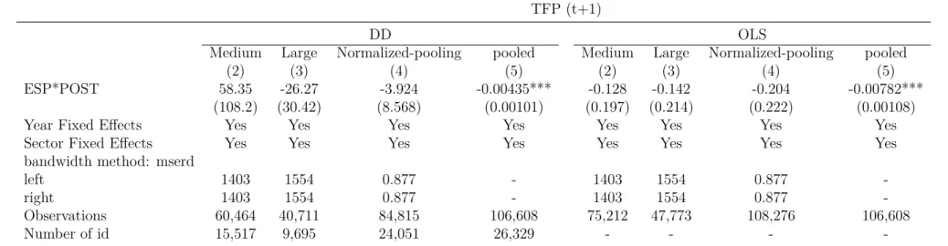
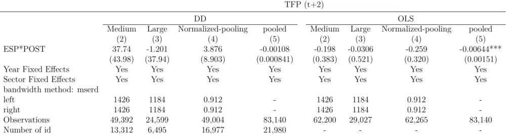
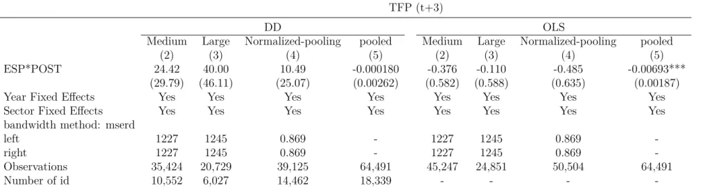
On Tables 1.9, 1.10 and 1.11 we exhibit ESP’s impact on total factor productivity 1, 2 and 3 years after receiving the grant. The main results are derived for the pooled approach, summarizing the general main findings after controlling for firm heterogeneity (column (5)), the mean effect is about -0,43% decrease in TFP in subsequent year for the subsidized firms relative to non-subsidized ones. OLS columns indicate that although SMEs beneficiaries show a decrease in TFP following the grant but it’s not permanent

18

Only -mserd- bandwidth is presented for the sake of brevity and to conserve space. Hence, only the summary of results are showed. For each firm size, the distance around zero should be calculated as:

(28)

in t+2 and t+3. For both Medium and Large enterprises, the effects are not statistically different from zero. The results remain unchanged when we try two different MSE-optimal bandwidth selectors on each cutoffs side.

The impact on wage per worker, as showed in Table 1.12, does not change on subsequent year after the grant. Again, even normalized-pooled effect is not robust to year and sector fixed effect inclusions. Two years after ESP grant, as presented in Table 1.13 firms does not show any change on wage per worker compared to non-subsidized ones.

For sales per worker in t+1, in turn, average estimates reported on for normalized-pooling approach from Table 1.14 shows a decrease for subsidized firms relative to baseline. However, this effect vanishes two and three year after the grant as Tables 1.15 and 1.16 show. Estimations using other bandwidths reinforce the results. Finally, Table 1.17 show that without controlling for other firm sizes, it means, just normalizing (all) gross revenue to zero and polling all firms together, the probability of firm’s death decreases substantially after controlling for macroeconomic shocks and sector-variant effects such as productivity differences. Looking up for cutoff-individual effects shows that results are not different from zero or robust to year/sector fixed effects inclusions.

Grant impact on quitters is consistent with Howell (2016). In her case, however, exit is related to IPO or acquisition which we cannot infer from our results. In addition, Chor and Manova (2012) show that overall credit conditions were important on explaining how the global financial crisis affected trade volumes. Such impact was more pronounced on sectors that require extensive external financing, have limited access to trade credit, or have few collateralizable assets.

1.5.1 Robustness Tests

This section addresses validity of the empirical results. To test the sensitivity of our results we follow two approaches. First, we test whether a hypothetical cutoff at R$ 21 million delivers significant results. If it does so, our identification hypothesis is not consistent as it relies on changes on firm’s counterpart funding. R$ 21 million is far away from both R$ 10.5 mi and R$ 60 mi. So, we expect that firms with gross revenue around R$ 21mi do not improve its competitiveness regarding those near all other cutoffs.

(29)

the validity of instruments.

Finally, we assess whether changes on mandatory financial counterpart affect the results. Tables 1.21 – 1.23 report differences in discontinuities estimates following Equation 1.7 with an additional post-treatment set in the year 2008. Tables 1.24 – 1.26 present OLS estimates as baseline. Reinforcing results presented above, there is no evidence of ESP’s impact for subsidized firms on target outcomes.

The main policy implication is that ESP’s design is not affecting its original goals such as firm performance or access to foreign market. This is due to the fact that projects are designed to last for 36 months. So, the first firms signed contracts in 2007 and project were expected to last until 2010. It may be the case that performance variables of enterprises are affected only after the entry of new products and processes been released. Moreover, FINEP changes its guidelines in 2010, restricting even more the set of firms eligible to grants by publishing only thematic public calls. Maybe this could be due to an acknowledgment that the ESP’s design needed to be revised. However, to test whether this is true we should rely on a larger time span.

1.6 Concluding remarks

This paper analyzes the role of public subsidies on innovation effort by firms, assessing the effectiveness of such policies on target firm performance. We evaluate the Economic Subvention Program, managed by FINEP in Brazil during 2006-2009. Investment promotion policies are broadly recognized to overcome the under-provision of innovative activities with respect to the social optimum.

To what extent do the findings agree with the FINEP’s intended goals? Access to ESP grant is open to all firms. Thus, if a particular firm wants to innovate, there is no (a priori) reason to not apply for a free grant such as ESP. Instrumenting for counterpart funding (proxy for innovation cost) to reduce the self–selection and endogeneity bias, we estimate the ESP’s effect on a wide variety of firm performance outcomes.

(30)

policy is ruled out by exploring changes on ESP assignment rules that directly aﬀect these ﬁrms.

(31)

Figure 1.1: log(gross operating revenue) distribution

(32)

Table 1.1: Mandatory (minimum) Financial Compensation as % of Grants

Firm size 2006 2007 2008 2009

Micro-enterprise 5 5 5 5

Small 20 20 20 20

Medium 40 40 100 100

Large 60 60 200 200

Notes: tHE Financing counterpart is set according to the firm’s previous year gross revenue. FINEP classifies as micro-enterprise those whose revenues are strictly less than R$ 2.4 million; as small whose gross revenues are greater than R$ 2.4 mi and strictly less than R$ 10.5 mi; as medium those with for revenues greater than R$ 10.5 and strictly less than R$ 60mi; as large those with revenues greater than R$ 60 million.

Table 1.2: FINEP’s actual disbursement and ESP’s budget Year # of projects_ﬁnanced Total budget, in_{R$1000 (A)}

Eﬀective disbursements

(share of A)

(Mean) Grant by project, in

R$ 1000

2006 195 R$ 300,000.00 122% R$ 1,877.43

2007 116 R$ 450,000.00 31% R$ 1,215.64

2008 209 R$ 450,000.00 95% R$ 2,045.53

2009 231 R$ 450,000.00 94% R$ 1,839.22

Source: FINEP/APLA. Author’s elaboration.

Table 1.3: Demand for grants - FINEP Year # Applications

Resources demanded (R$ million)

Qualiﬁed (%) Approved (%)

2006 1,099 1,842 N/A N/A

2007 2,567 4,123 21% 7%

2008 2,664 6,025 29% 9%

2009 2,558 5,202 49% 10%

Source: FINEP/APLA. Author’s elaboration.

Table 1.4: Treated vs. non-treated - ESP

# non-beneficiaries obs. # beneficiaries obs. Total _{to annual gross revenue (in R$ 1000)}Firm size definition according

Micro-enterprise 125671 13 125684 [0,2400]

Small 75584 133 75717 (2400,10500]

Medium 59107 244 59351 (10500,60000]

Large 21388 232 21620 [60000,∞)

Total 281750 622 282372

(33)

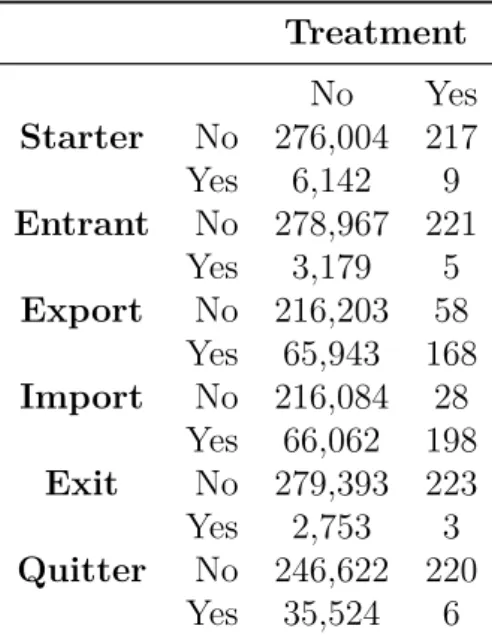
Table 1.5: Characteristics of ﬁrst-time treatment Treatment

No Yes

Starter No 276,004 217

Yes 6,142 9

Entrant No 278,967 221

Yes 3,179 5

Export No 216,203 58 Yes 65,943 168 Import No 216,084 28

Yes 66,062 198 Exit No 279,393 223

Yes 2,753 3

Quitter No 246,622 220 Yes 35,524 6

Notes: First-time treatment refer to the first year that firm receives the subsidy. Number of treated: 226. Number of untreated: 282,146. Definitions are described on Table 1.6.

Table 1.6: Outcomes

Outcome Description

exit =1 if ﬁrm exported in t-1, exported in t and did not export in t+1 entrants =1 if ﬁrm did not export in t-1 and exported in t and t+1

starter =1 if ﬁrm did not export in t-1 and export em t (less restrictive than_entrants) f1_tfp total factor productivity t+1

f2_tfp total factor productivity t+2 f3_tfp total factor productivity t+3

f1_lnw wage per worker t+1

f2_lnw wage per worker t+2

f1_sales_per_worker sales per worker t+1 f2_sales_per_worker sales per worker t+2 f3_sales_per_worker sales per worker t+3

(34)

Table 1.7: Outcome: Pr(exit export market)

Pr(exit export market)

DD OLS

Medium Large Normalized-pooling pooled Medium Large Normalized-pooling pooled

(1) (2) (3) (4) (1) (2) (3) (4)

ESP*POST 1.453 -2.627 0.255 4.05e-05 2.93e-05 -0.0146*** -0.00820*** 0.000184*** (10.45) (5.009) (0.383) (6.99e-05) (0.00542) (0.00203) (0.00250) (5.31e-05)

Year Fixed Eﬀects Yes Yes Yes Yes Yes Yes Yes Yes

Sector Fixed Eﬀects Yes Yes Yes Yes Yes Yes Yes Yes

bandwidth method: mserd

left 1658 1481 0.806 - 1658 1481 0.806

-right 1658 1481 0.806 - 1658 1481 0.806

-Observations 104,833 53,997 189,557 161,112 133,430 64,066 256,821 161,112

Number of id 25,052 12,181 44,009 37,495 - - -

(35)

Table 1.8: Outcome: Pr(entry and remain as exporter)

Entrant: Pr(entry and remain exporter)

DD OLS

(2) (3) (4) (5) (2) (3) (4) (5)

ESP*POST 14.25 -11.89 -2.221*** -4.70e-05 0.0142 -0.00574 -0.000697 -3.88e-05

(15.88) (10.86) (0.468) (9.88e-05) (0.0103) (0.00878) (0.00516) (3.68e-05)

left 0.954 1457 0.485 - 0.954 1457 0.485

-right 0.954 1457 0.485 - 0.954 1457 0.485

-Observations 71,147 53,012 154,100 175,924 89,428 62,863 206,681 175,924

Number of id 18,354 11,985 40,342 40,658 - - -

(36)

Table 1.9: Outcome: Total Factor Productivity (t+1)

TFP (t+1)

DD OLS

(2) (3) (4) (5) (2) (3) (4) (5)

ESP*POST 58.35 -26.27 -3.924 -0.00435*** -0.128 -0.142 -0.204 -0.00782***

(108.2) (30.42) (8.568) (0.00101) (0.197) (0.214) (0.222) (0.00108)

left 1403 1554 0.877 - 1403 1554 0.877

-right 1403 1554 0.877 - 1403 1554 0.877

-Observations 60,464 40,711 84,815 106,608 75,212 47,773 108,276 106,608

Number of id 15,517 9,695 24,051 26,329 - - -

(37)

TFP (t+2)

DD OLS

(2) (3) (4) (5) (2) (3) (4) (5)

ESP*POST 37.74 -1.201 3.876 -0.00108 -0.198 -0.0306 -0.259 -0.00644***

(43.98) (37.94) (8.903) (0.000841) (0.383) (0.521) (0.320) (0.00151)

left 1426 1184 0.912 - 1426 1184 0.912

-right 1426 1184 0.912 - 1426 1184 0.912

-Observations 49,392 24,599 49,004 83,140 62,200 29,027 62,265 83,140

Number of id 13,312 6,495 16,977 21,980 - - -

(38)

TFP (t+3)

DD OLS

(2) (3) (4) (5) (2) (3) (4) (5)

ESP*POST 24.42 40.00 10.49 -0.000180 -0.376 -0.110 -0.485 -0.00693***

(29.79) (46.11) (25.07) (0.00262) (0.582) (0.588) (0.635) (0.00187)

left 1227 1245 0.869 - 1227 1245 0.869

-right 1227 1245 0.869 - 1227 1245 0.869

-Observations 35,424 20,729 39,125 64,491 45,247 24,851 50,504 64,491

Number of id 10,552 6,027 14,462 18,339 - - -

(39)

Table 1.12: Outcome: Wage per worker (t+1)

Wage per worker (t+1)

DD OLS

(2) (3) (4) (5) (2) (3) (4) (5)

ESP*POST 6.982 28.14 1.211 -0.000174 0.232* 0.367*** 0.560*** 0.00224***

(32.61) (22.35) (1.976) (0.000530) (0.118) (0.106) (0.0838) (0.000386)

left 1198 1207 0.587 - 1198 1207 0.587

-right 1198 1207 0.587 - 1198 1207 0.587

-Observations 68,004 33,850 85,458 122,417 85,119 39,637 110,216 122,417

Number of id 17,545 8,398 27,444 30,289 - - -

(40)

Table 1.13: Outcome: Wage per worker (t+2)

Wage per worker (t+2)

DD OLS

(2) (3) (4) (5) (2) (3) (4) (5)

ESP*POST 30.36 14.82 1.569 -0.000846 0.249* 0.447*** 0.539*** 0.00218***

(49.27) (20.09) (2.742) (0.000698) (0.134) (0.152) (0.152) (0.000477)

left 1083 1020 0.573 - 1083 1020 0.573

-right 1083 1020 0.573 - 1083 1020 0.573

-Observations 50,764 22,780 57,653 110,230 64,196 26,839 74,621 110,230

Number of id 14,120 6,267 21,135 28,838 - - -

(41)

Table 1.14: Outcome: Sales per worker (t+1)

Sales per worker (t+1)

DD OLS

(2) (3) (4) (5) (2) (3) (4) (5)

ESP*POST 63.66 -4.580 -8.029** -0.000547 0.250*** 0.216 0.638*** 0.00575***

(78.30) (11.46) (4.085) (0.00164) (0.0424) (0.145) (0.128) (0.000355)

left 0.867 0.525 0.328 - 0.867 0.525 0.328

-right 0.867 0.525 0.328 - 0.867 0.525 0.328

-Observations 51,945 13,957 29,447 29,447 64,574 16,231 37,120 109,556

Number of id 14,500 4,318 15,423 15,423 - - -

(42)

DD OLS

(2) (3) (4) (5) (2) (3) (4) (5)

ESP*POST 71.89 -3.376 -22.19* -0.00115 0.283*** 0.248** 0.491*** 0.00774***

(179.4) (6.768) (11.86) (0.00103) (0.0459) (0.0981) (0.0906) (0.000460)

left 0.868 0.930 0.375 - 0.868 0.930 0.375

-right 0.868 0.930 0.375 - 0.868 0.930 0.375

-Observations 41,813 20,496 30,478 89,792 52,622 24,101 38,885 89,792

Number of id 12,312 5,745 14,663 23,918 - - -

(43)

DD OLS

(2) (3) (4) (5) (2) (3) (4) (5)

ESP*POST 9.845 -0.105 -13.31 -0.00108 0.270*** 0.259*** 0.607*** 0.00439***

(19.31) (7.339) (9.943) (0.00168) (0.0461) (0.0920) (0.0814) (0.000464)

left 0.959 1050 0.441 - 0.959 1050 0.441

-right 0.959 1050 0.441 - 0.959 1050 0.441

-Observations 36,158 18,780 22,363 78,183 46,407 22,499 29,000 78,183

Number of id 11,267 5,702 11,837 22,329 - - -

(44)

Table 1.17: Outcome: Pr(leave the market)

Quit: Pr(leave the market)

DD OLS

(2) (3) (4) (5) (2) (3) (4) (5)

ESP*POST 3.776 13.22 -12.99*** 0.000393 -0.0585*** -0.0844*** -0.0672*** 0.00106***

(4.924) (29.88) (3.106) (0.000323) (0.00757) (0.00583) (0.00978) (0.000141)

left 0.584 1005 0.404 - 0.584 1005 0.404

-right 0.584 1005 0.404 - 0.584 1005 0.404

-Observations 45,563 35,184 74,262 138,038 56,659 41,437 96,255 138,038

Number of id 13,873 8,486 27,844 32,495 - - -

(45)

Table 1.18: Falsiﬁcation test: Placebo at R$21 million.

Pr(exit export market) Entrant: Pr(entry and remain exporter) Pr(leave the market)

ESP*POST -20.54 -10.28 78.70

(49.19) (77.75) (181.2)

Year Fixed Eﬀects Yes Yes Yes

Sector Fixed Eﬀects Yes Yes Yes

Observations 14,633 20,470 27,212

Number of id 6,539 7,755 9,024

(46)

Table 1.19: Falsiﬁcation test: Placebo at R$21 million.

Wage per worker (t+1) Wage per worker (t+2) Sales per worker (t+1) Sales per worker (t+2) Sales per worker (t+3)

ESP*POST 29.29 -2.148 12.95 27.28 -58.87

(33.84) (41.78) (151.5) (35.54) (138.6)

Year Fixed Eﬀects Yes Yes Yes Yes Yes

Sector Fixed Eﬀects Yes Yes Yes Yes Yes

Observations 22,180 12,798 17,168 18,524 14,256

Number of id 7,637 5,323 6,636 6,630 5,606

(47)

Table 1.20: Falsiﬁcation test: Placebo at R$21 million. TFP (t+1) TFP (t+2) TFP (t+3)

ESP*POST 7.620 73.84 -452.8

(56.93) (102.7) (1,192)

Observations 28,714 14,551 11,615

Number of id 8,473 5,444 4,672

(48)

Table 1.21: Eﬀect of cutoﬀ changing in 2008

Pr(exit export market) Pr(start export) Entrant Pr(entry and remain exporter) Pr(leave the market)

ESP*POST 11.10 -12.05 -15.03 -21.23

(10.25) (21.09) (15.88) (38.72)

Year Fixed Eﬀects Yes Yes Yes Yes

Sector Fixed Eﬀects Yes Yes Yes Yes

Observations 91,953 62,039 75,139 39,480

Number of id 33,885 27,105 30,613 19,779

(49)

TFP (t+1) TFP (t+2) Wage per worker (t+1)

ESP*POST 34.35 18.77 -0.142

(33.42) (16.55) (17.43)

Observations 32,057 14,442 36,001

Number of id 15,810 9,597 18,668

(50)

Wage per worker (t+2) Sales per worker (t+1) Sales per worker (t+2)

ESP*POST -11.27 391.8 -17.34

(17.31) (2,401) (17.16)

Observations 18,897 13,920 10,805

Number of id 12,687 9,250 7,895

(51)

Table 1.24: Eﬀect of cutoﬀ changing in 2008 - OLS estimates

Pr(exit export market) Pr(start export) Entrant Pr(entry and remain exporter) Pr(leave the market)

ESP*POST -0.00851*** 0.000872 0.00264 -0.0606***

(0.00163) (0.0137) (0.00730) (0.0104)

Year Fixed Eﬀects Yes Yes Yes Yes

Sector Fixed Eﬀects Yes Yes Yes Yes

Observations 115,632 76,967 93,862 48,547

(52)

TFP (t+1) TFP (t+2) Wage per worker (t+1)

ESP*POST 0.0207 -0.653** 0.613***

(0.987) (0.307) (0.102)

Observations 36,472 16,333 42,705

(53)

Wage per worker (t+2) Sales per worker (t+1) Sales per worker (t+2)

ESP*POST 0.611*** 0.584*** 0.506***

(17.31) (2,401) (17.16)

Observations 22,428 16,332 12,749

(54)

Chapter 2 On the complementarity between

exporting and innovation

Abstract

This paper aims to study the complementarity between exporting and innovation in the Brazilian industry. Do firms become more prone to invest in innovation after becoming an exporter? We tackle this issue by analyzing Brazilian firm level data from 1998-2011 linking three databases through a firm identifier.We use propensity score kernel matching combined with difference-in-differences approach to help deal with endogenous exporting, sunk exporting costs and common macroeconomic shocks across industries. The findings show that exporting is associated with further innovation expenditures, although this effect vanishes two years after entry in the export market.

Keywords: innovation; firm-level data; learning by exporting; Kernel propensity score; differences-in-differences.

JEL Classiﬁcation: D22, F14, F23, O3.

Acknowledgements

The author wishes to acknowledge the invaluable comments from Emanuel Ornelas and João Paulo Pessoa. All remaining errors are responsibility of the author.