Jan Zizka et al. (Eds) : CCSIT, SIPP, AISC, CMCA, SEAS, CSITEC, DaKM, PDCTA, NeCoM - 2016 pp. 201–218, 2016. © CS & IT-CSCP 2016 DOI : 10.5121/csit.2016.60118
Pedro Martins, Maryam Abbasi, Pedro Furtado
Department of Informatics, University of Coimbra, Portugal
[email protected], [email protected], [email protected]
A
BSTRACTIn this paper we investigate the problem of providing scalability to near-real-time ETL+Q (Extract, transform, load and querying) process of data warehouses. In general, data loading, transformation and integration are heavy tasks that are performed only periodically during small fixed time windows.
We propose an approach to enable the automatic scalability and freshness of any data warehouse and ETL+Q process for near-real-time BigData scenarios. A general framework for testing the proposed system was implementing, supporting parallelization solutions for each part of the ETL+Q pipeline. The results show that the proposed system is capable of handling scalability to provide the desired processing speed.
K
EYWORDSScalability, ETL, freshness, high-rate, performance, parallel processing, distributed systems, database, load-balance, algorithm
1. I
NTRODUCTION
ETL tools are special purpose software used to populate a data warehouse with up-to-date, clean records from one or more sources. The majority of current ETL tools organize such operations as a workflow. At the logical level, the E (Extract) can be considered as a capture of data-flow from the sources with more than one high-rate throughput. T (Transform) represents transforming and cleansing data in order to be distributed and replicated across many processes and ultimately, L(Load) the data into data warehouses to be stored and queried. For implementing these type of systems besides knowing all of these steps, the acknowledgement of user regarding the scalability issues is essential.
After extraction, data must be re-directed and distributed across the available transformation nodes, again since transformation involves heavy duty tasks (heavier than extraction), more than one node should be present to assure acceptable execution/transformation times. Once again more new data distribution policies must be added. After the data is transformed and ready to be loaded, the load period time and a load time control must be scheduled. This means that the data have to be held between the transformation and loading process in some buffer. Eventually, regarding the data warehouse schema, the entire data will not fit into a single node, and if it fits, it will not be possible to execute queries within acceptable time ranges. Thus, more than one data warehouse node is necessary with a specific schema which allows to distribute, replicate, and query the data within an acceptable time frame.
In this paper we study how to provide parallel ETL+Q scalability with ingress high-data-rate in big data warehouses. We propose a set of mechanisms and algorithms to parallelize and scale each part of the entire ETL+Q process, which later will be included in an auto-scale (in and out) ETL+Q framework. The presented results prove that the proposed mechanisms are able to scale when necessary.
In Section 2 we present some relevant related-work in the field. Section 3 describes the architecture of the proposed system, Section 4 explains the main algorithms which allow to scale-out when necessary. Section 5 shows the experimental results obtained when testing the proposed system. Finally, Section 6 concludes the paper and discusses future work.
2. R
ELATED
W
ORK
Works in the area of ETL scheduling includes efforts towards the optimization of the entire ETL workflows [8] and of individual operators in terms of algebraic optimization; e.g., joins or data sort operations.
The work [4] deals with the problem of scheduling ETL workflows at the data level and in particular scheduling protocols and software architecture for an ETL engine in order to minimize the execution time and the allocated memory needed for a given ETL workflow. The second aspect in ETL execution that the authors address is how to schedule flow execution at the operations level (blocking, non-parallelizable operations may exist in the flow) and how we can improve this with pipeline parallelization [3].
The work [6] focuses on finding approaches for the automatic code generation of ETL processes which is aligning the modeling of ETL processes in data warehouse with MDA (Model Driven Architecture) by formally defining a set of QVT (Query, View, Transformation) transformations.
ETLMR [5] is an academic tool which builds the ETL processes on top of Map-Reduce to parallelize the ETL operation on commodity computers. ETLMR does not have its own data storage (note that the offine dimension store is only for speedup purpose), but is an ETL tool suitable for processing large scale data in parallel. ETLMR provides a configuration file to declare dimensions, facts, User Defined Functions (UDFs), and other run-time parameters.
fault-tolerance, by considering various techniques. In this approach partitioning can be based on round-robin (RR), hash (HS), range (RG), random, modulus, copy, and others [9].
In [2] the authors describe Liquid, a data integration stack that provides low latency data access to support near real-time in addition to batch applications. It supports incremental processing, and is cost-efficient and highly available. Liquid has two layers: a processing layer based on a statefull stream processing model, and a messaging layer with a highly-available publish / subscribe system. The processing layer (i) executes ETL-like jobs for different back-end systems according to a stateful stream processing model [1]; (ii) guarantees service levels through resource isolation; (iii) provides low latency results; and (iv) enables incremental data processing. A messaging layer supports the processing layer. It (i) stores high-volume data with high availability; and (ii) offers rewindability, i.e. the ability to access data through meta-data annotations. The two layers communicate by writing and reading data to and from two types of feeds, stored in the messaging layer.
Related problems studied in the past include the scheduling of concurrent updates and queries in real-time warehousing and the scheduling of operators in data streams management systems. However, we argue that a fresher look is needed in the context of ETL technology. The issue is no longer the scalability cost/price, but rather the complexity it adds to the system. Previews presented recent works in the field do not address in detail how to scale each part of the ETL+Q and do not regard the automatic scalability to make ETL scalability easy and automatic. The authors focus on mechanisms to improve scheduling algorithms and optimizing work-flows and memory usage. In our work we assume that scalability in number of machines and quantity of memory is not the issue, we focus on offering scalability for each part of the ETL pipeline process, without the nightmare of operators relocation and complex execution plans. Our main focus is on scalability based on generic ETL process to provide the users desired performance with minimum complexity and implementations. In addition, we also support queries execution.
3. A
RCHITECTURE
In this section we describe the main components of the proposed architecture for ETL+Q scalability. Figure 1 shows the main components to achieve automatic scalability.
• All components from (1) to (7) are part of the Extract, Transform, Load and query (ETL+Q) process.
• The "Automatic Scaler" (13), is the node responsible for performance monitoring and scaling the system when it is necessary.
• The "Configuration file" (12) represents the location where all user configurations are defined by the user.
Figure 2: Total automatic ETL+Q scalability
• The "Configuration API" (10), is an access interface which allows to configure each part of the proposed Universal Data Warehouse architecture, automatically or manually by the user.
• Finally the "Scheduler" (14), is responsible for applying the data transfer policies between components (e.g. control the on-demand data transfers).
Figure 1: Automatic ETL+Q scalability
All these components when set to interact together are able to provide automatic scalability to the ETL and to the data warehouses processes without the need for the user to concern about its scalability or management.
Paralelization approach
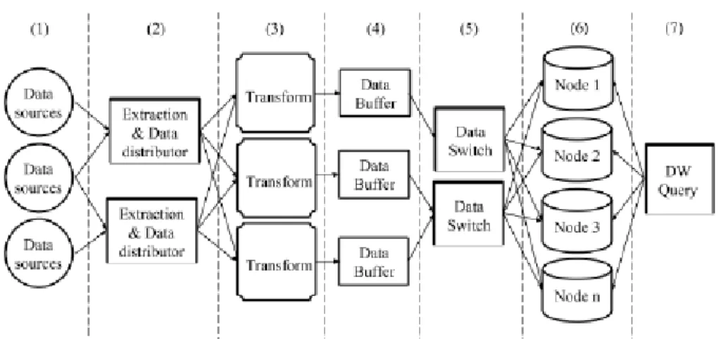
Figure 2 depicts the main processes needed to support total ETL+Q scalability.
2) The data distributor(s) is responsible for forwarding or replicating the raw data to the transformer nodes. The distribution algorithm to be used is configured and enforced in this stage. The data distributors (2) should also be parallelizable if needed, for scalability reasons.
3) In the transformation nodes the data is cleaned and transformed to be loaded into the data warehouse. This might involve data lookups to in-memory or disk tables and further computation tasks. The transformation is parallelized for scalability reasons.
4) The data buffer can be in memory, disk file (batch files) or both. In periodically configured time frames/periods, data is distributed across the data warehouse nodes.
5) The data switches are responsible to distribute (pop/extract) data from the "Data Buffers" and set it for load into the data warehouse, which can be a single-node or a parallel data warehouse depending on configured parameters (e.g. load time, query performance).
6) The data warehouse can be in a single node, or parallelized by many nodes. If it is parallelized, the "Data Switch" nodes will manage data placement according to configurations (e.g. replication and distribution). Each node of the data warehouse loads the data independently from the batch files.
7) Queries are rewritten and submitted to the data warehouse nodes for computation. The results are then merged, computed and returned.
The main concept we propose are the individual ETL+Q scalability mechanisms of each part of the ETL+Q pipeline. By offering solution to scale each part independently, we provide a solution to obtain configurable performance.
4. D
ECISION
A
LGORITHMS
F
OR
S
CALABILITY
P
ARAMETERS
In this section we define the scalability decision methods as well as the algorithms which allow the framework to automatically scale-out and scale-in.
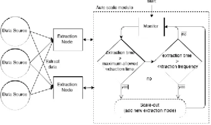
Extraction & data distributors - Scale-out
Extraction & data distributors- Scale-in
Figure 3: Extraction algorithm-scale-out
To save resources when possible, nodes that perform the data extraction from the sources can be set in standby or removed. This decision is made based on the last execution times. If previous execution times of at least two or more nodes are less than half of the maximum extraction time (or if the maximum extraction time is not configured, the frequency), minus a configured variation parameter (X), one of the nodes is set on standby or removed, and the other one takes over. Flowchart 4 describes the applied algorithm to scale-in.
Transform - Scale-out
The transformation process is critical, if the transformation is running slow, data extraction at the referred rate may not be possible, and information will not be available for loading and querying when necessary. The transformation step has an important queue used to determine when to scale the transformation phase. If this queue reaches a limit size (by default 50%), then it is necessary to scale, because the actual transformer node(s) is not being able to process all the data that is arriving. The size of all queues is analyzed periodically. If this size at a specific moment is less than half of the limit size for at least two nodes, then one of those nodes is set on standby or removed. Flowchart 5, describes the algorithm used to scale-out and scale-in.
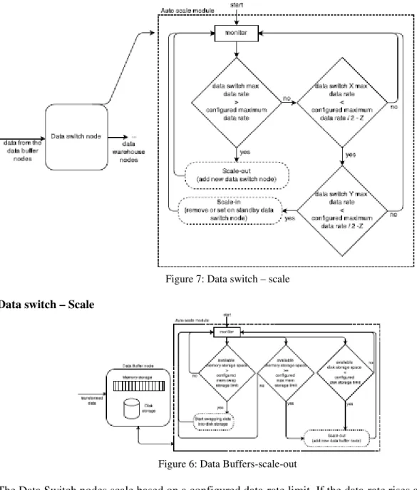
Data buffer - Scale
Figure 5: Transformation - scale-in and scale-out
Figure 7: Data switch – scale
Data switch – Scale
Figure 6: Data Buffers-scale-out
The Data Switch nodes scale based on a configured data-rate limit. If the data-rate rises above the configured limit the data switch nodes are set to scale-out. The data switches can also scale-in, in this case the system will allow it if the data-rate is less than the configured maximum by at least 2 nodes, minus a Z configured variation, for a specific time. Flowchart 7 describes the used algorithm to scale the data switch nodes.
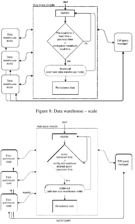
Data Warehouse – Scale
The data warehouse scalability is not only based on the load & integration speed requirements, but also on the queries desired maximum execution time. After each query execution, if the query time to the data warehouse is more than the configured maximum desired query execution time, then the data warehouse is set to scale-out. The Flowchart 9 describes the algorithm used to scale the data warehouse based on the average query execution time.
Figure 8: Data warehouse – scale
The data warehouse nodes scale-in is performed if the average query execution time and the average load time respect the conditions 1 and 2 (where n represents the number of nodes):
and
Every time the data warehouse scales-out or scales-in the data inside the nodes needs to be re-balanced. The default re-balance process to scale-out is based on the phases: Replicate dimension tables; Extract information from nodes; Load the extracted information into the new nodes. Scale-in process is more simple, data just needs to be extracted and loaded across the available nodes as if it is new data.
5. E
XPERIMENTAL
S
ETUP
AND
R
ESULTS
In this section we describe the experimental setup, and experimental results to show that the proposed system, AScale, is able to scale and load balance data and processing.
5.1 Experimental Setup
In this section we describe the used testbed. The experimental tests were performed using 12 computers, denominated as nodes, with the following characteristics: Processor Intel Core i5-5300U Processor (3M Cache, upto 3.40 GHz); Memory 16GB DDR3; Disk: western digital 1TB 7500rpm; Ethernet connection 1Gbit/sec; Connection switch: SMC SMCOST16, 16 Ethernet ports, 1Gbit/sec.
The 12 nodes were formatted before the experimental evaluation and installed with: Windows 7 enterprise edition 64 bits; Java JDK 8; Netbeans 8.0.2; Oracle Database 11g Release 1 for Microsoft Windows (X64) - used in each data warehouse nodes; PostgreSQL 9.4 - used for look ups during the transformation process; TPC-H benchmark - representing the operational log data used at the extraction nodes. This is possible since TPC-H data is still normalized; SSB benchmark - representing the data warehouse. The SSB is the star-schema representation of TPC-H data.
5.2 Automatic scalability
In this section we describe the scalability tests made to the full auto-scale ETL framework. We demonstrate scale-out and scale-in ability of the proposed framework using the proposed algorithms. Consider the following scenario:
• The transformation process consists of transforming the TPC-H relational model into a star-schema model, which is the SSB benchmark. This process involves heavy computational memory, temporary storage of large amounts of data, look-ups and data transformations to assure consistency;
• The data warehouse tables schema consist on the same schema from SSB benchmark. Replication and partitioning is assured by AScale, whereas, dimension tables are replicated and fact tables are partitioned across the data warehouse nodes.
• The E, T and L were set to perform every 2 seconds, and cannot last more than 1 second. Thus the ETL process will last at the worst case 3 seconds total;
• The load process was made in batches of 100MB maximum;
• All default configurations of other components were set to use the default AScale configurations.
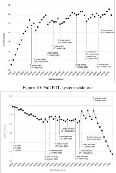
Figure 10: Full ETL system scale-out
Figure 10 and 11 show how the proposed auto-scale ETL framework scales to deliver the configured ETL execution time, while the data rate increases/decreases. In the charts the X axis is represented the data-rate per second, from 10.000 to 500.000 rows per second and the Y axis is the ETL time expressed in seconds; The system objective was set to deliver the ETL process in 3 seconds; In the charts we also represent the scale-out and scale-in of each part of the framework, by adding and removing nodes when necessary. Note that If we set a lower execution time the framework will scale-out faster. If the execution time is higher (e.g. 3 minutes) the framework will scale later if more performance is necessary at any module.
Scale-out results from Figure 10 show that, as the data-rate increases and parts of the ETL pipeline become overloaded, by using all proposed monitoring mechanisms in each part of the AScale framework, each individual module scales to offer more performance where necessary. In Figure 10, we point each scaled-out module.
Note that in some stages of the tests the 3 seconds limit execution time was exceeded in 0.1, 0.2 seconds. This happened due to the high data-rate usage of the network connecting all nodes that is not being accounted for the purposes of our tests.
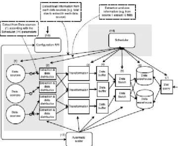
Scale-in results from Figure 11 show the moment when the current number of nodes are no longer necessary to assure the desired performance, and some nodes could be removed to be set as ready node in stand-by and be used in other parts to assure the ETL configured time.
When comparing the moments of scale-out and scale-in, it is possible to observe that the proposed framework scales-out much faster than it scales-in. When a scale-in can be applied it is performed in a later stage than a scale-out.
5.3 Data extraction nodes scalability
Figure 12: Sources to extraction
Figure 12 shows the scheduler based extraction approach to extract data, where the "automatic scaler" (13) orders the nodes to extract data from sources (scheduler based extraction policy). Considering "data sources" (1) generate high rate data and "extraction nodes" (2) extract the generated data, when the dataflow is too high a single data node cannot handle all ingress data. In this section we study how the extraction nodes scale to handle different data-rates. The maximum allowed extraction time was set to 1 second. Extraction frequency was set to every 3 seconds.
In Figure 13 we have in the left Y axis, the average extraction time in seconds; in the right Y axis, the number of nodes; The X axis is the datarate; Black line represents the extraction time; Grey line represents the number of nodes as they scale-out. It is possible to see that every time the extraction takes too much time (more than 1 second as configured) a new node is added (from the ready-nodes pool). After the new node added, more nodes are being used to extract data from the same number of sources, so the extraction time improves. As we increase the data-rate, the extraction time becomes higher until it reaches more than 1 second, and another node is added.
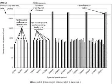
5.4 Transformation scalability
During the ETL process, after data is extracted, it is set for transformation. Because this process is computationally heavy, it is necessary to scale the transformation nodes to assure that all data is processed without delays. Each transformation node has an entrance data queue, for ingress data. The "automatic scaler" (13) monitors all queues, once it detects that a queue is full and above a certain configured threshold it starts the scale process, this means that Rateextract
Ratetransform
Figure 14: Automatic transformation scalability. 60 minutes processing per data-rate.
In Figure 14 you can see in Y axis, the average queue size in number of rows; in X axis, the data rate in rows per second; Each plotted bar represents the average transformation node queue size (up to 4 nodes); Each measure represents the average queue size of 60 seconds run. As it displays the moments when the queue size of the transformation nodes increase above the configured limit size, a new transformation node is added and data is distributed by all nodes to support the increasing data-rate.
5.5 Data Buffer nodes
This nodes hold the transformed data until it is loading into the data warehouse. The data buffers have the following configuration: Generation data rate speed 350.000 rows per second (i.e. transformation output data rate); Available memory storage 10.000MB (50% = 5.000MB); Available disk storage 1TB. We consider only the data generation/producer, there is no data "consumer", so the buffer must hold all ingress data.
Figure 15 shows: X axis represents the time; Left Y axis represents the memory size; Right Y axis represents the disk storage size; The bars represent the memory usage; Continuous line represent the total data size in disk, being swapped from memory. The chart shows the buffer nodes scalingout. When 50% of the memory size is used, data starts being swapped into disk. However, if the disk cannot handle all ingress data and the memory reaches the maximum limit size, a new node is added. After a new node added, data is distributed by both nodes. This makes the data-rate at each node less (at least half) and then the disk from the first node can empty the memory back to 50%. After this point each time 50% of the maximum configured memory is reached, data will swap into disk to free the memory.
5.6 Data warehouse scalability
In this section we test the data warehouse scalability, which can be triggered either by the load process (because it is taking too long), or because the query execution is taking more time than the desired response time.
To test the data warehouse nodes load scalability we set the load method by using batch files of maximum 100Mb. The maximum allowed load time was set to 60 seconds. Each time a data warehouse node is added, we show the data size that was moved into the new node and the required time in seconds to re-balance the data. All load and re-balance times include the execution of Pre-load tasks (i.e. destroy all indexes and views) and Pos-load tasks (i.e. rebuild indexes and update views). If the maximum configured load time is exceeded more than 60 seconds, the data warehouse is set to be scaled.
Figure 16: Data warehouse load scalability
Experimental results in this chart shows how the load performance degrades as the data size increases and how it improves when a new node is added. After a new node added performance improves below the maximum configured limit. Note that every time a new node was added, the data warehouse required to be re-balanced (data was evenly distributed by the nodes).
5.7 Query scalability
When running queries, if the maximum desired query execution time (i.e. configured parameter) is exceeded, then the data warehouse is set to scale in order to offer more query execution performance. The following workloads were considered to test AScale query scalability, Workload 1 with 50GB total size, executing queries Q1.1, Q2.1, Q3.1, Q4.1 chosen randomly and with a desired execution time per query of 1 minute. Workload 2 with the same properties as workload 1 but, using 1 to 8 simultaneous sessions.
Figure 17: Data warehouse scalability, workload 1
Workload 1 studies how the proposed mechanisms scales-out the data warehouse when running queries. Workload 2 studies the scalability of the system when running queries and the number of simultaneous sessions (e.g. number of simultaneous users) increases. Both workloads were set with the objective of guaranteeing the maximum execution time per query of 60 seconds.
Query scalability - Workload 1
time). Once the average query time reaches under the configured desired execution time, the framework stops scaling the data warehouse nodes.
Query scalability - Workload 2
Figure 18 shows the experimental results for workload 2. Total data was 50GB. Left Y axis shows the average query execution time in seconds and right Y axis, the average data re-balance time in seconds (i.e. extract from nodes, load into new node, rebuild indexes and views). X axis shows the number of sessions, the data size per node and the number of nodes. The horizontal line over 60 seconds represents the desired query execution time. The last result does not respect the desired execution time because of the limited hardware resources for our tests, 12 nodes.The results show that while the number of simultaneous sessions increases the system scales the number of nodes in order to provide more performance. The query average execution time follows the configured parameters. We also plot the data rebalance time. Every time a new node is added data must be balanced by all data warehouse nodes, this includes, extract data from the existent nodes, load into the new node, and finally re-create all indexes and views (since indexes and views updates are done in parallel for all nodes, we update all indexes and views in the data warehouse simultaneously).
6. C
ONCLUSION
& F
UTURE
W
ORK
In this work we propose mechanisms and algorithms to achieve automatic scalability for complex ETL+Q, offering the possibility to the users to think solely in the conceptual ETL+Q models and implementations for a single server.
The tests demonstrate that the proposed techniques are able to scale-out automatically when more resources are required. Future work includes the comparison with other state-of-the-art tools and the development of drag and drop interface to make AScale available to public.
R
EFERENCES[1] R. Castro Fernandez, M. Migliavacca, E. Kalyvianaki, and P. Pietzuch. Integrating scale out and fault tolerance in stream processing using operator state management. In Proceedings of the 2013 ACM SIGMOD international conference on Management of data, pages 725{736. ACM, 2013.
[2] R. C. Fernandez, P. Pietzuch, J. Koshy, J. Kreps, D. Lin, N. Narkhede, J. Rao, C. Riccomini, and G.Wang. Liquid: Unifying nearline and offine big data integration. In Biennial Conference on Innovative Data Systems Research (CIDR), Asilomar, CA, USA, 01/2015 2015. ACM, ACM.
[3] R. Halasipuram, P. M. Deshpande, and S. Padmanabhan. Determining essential statistics for cost based optimization of an etl workflow. In EDBT, pages 307{318, 2014.
[4] A. Karagiannis, P. Vassiliadis, and A. Simitsis. Scheduling strategies for efficient etl execution. Information Systems, 38(6):927{945, 2013.
[6] L. Munoz, J.-N. Mazon, and J. Trujillo. Automatic generation of etl processes from conceptual models. In Proceedings of the ACM twelfth international workshop on Data warehousing and OLAP, pages 33{40. ACM, 2009.
[7] A. Simitsis, C. Gupta, S. Wang, and U. Dayal. Partitioning real-time etl workflows, 2010.
[8] A. Simitsis, K. Wilkinson, U. Dayal, and M. Castellanos. Optimizing etl workflows for fault-tolerance. In Data Engineering (ICDE), 2010 IEEE 26th International Conference on, pages 385{396. IEEE, 2010.