AUGMENTING DATA WAREHOUSING ARCHITECTURES WITH HADOOP

AUGMENTING DATA WAREHOUSING

ARCHITECTURES WITH HADOOP

Henrique José Rosa Dias

NOVA Information Management School

Instituto Superior de Estatística e Gestão de Informação

AUGMENTING DATA WAREHOUSING ARCHITECTURES

WITH HADOOP

by

Henrique Dias

Dissertation presented as partial requirement for obtaining the Master’s degree in Information Management, with a specialization in Information Systems and Technologies Management

Advisor:Professor Roberto Henriques, PhD.

DEDICATION

ACKNOWLEDGEMENTS

There were times when it seemed impossible, after a while it just became hard but, in the end, it was done. Looking back now, and despite all the challenges and difficulties, I would most certainly do it again!

If it is true that a big part of this journey is a lonely one, it is also true that it would not be the same if I did not have the help of the people that, somewhere along the road, came and pushed me forward. This list is extensive but I would like to use this opportunity to convey some special messages of gratitude.

Firstly, I would like to express my sincere gratitude to my advisor, professor Roberto Henriques, not only for his advices, support and very thorough review of this dissertation, but also because it was greatly due to his Big Data Applications class that my interest for the Big Data world began to materialize, and, ultimately, this led to my thesis subject choice. Most probably without his class this dissertation would never have happened.

I would also like to thank my manager at Xerox, Simon Hawkins, for his flexibility and understanding throughout this journey that, at times, revealed to be difficult to separate from my professional obligations, and, of course, for his precious help in overcoming my constant doubts related to writing in English.

ABSTRACT

As the volume of available data increases exponentially, traditional data warehouses struggle to transform this data into actionable knowledge. Data strategies that include the creation and maintenance of data warehouses have a lot to gain by incorporating technologies from the Big Data’s spectrum. Hadoop, as a transformation tool, can add a theoretical infinite dimension of data processing, feeding transformed information into traditional data warehouses that ultimately will retain their value as central components in organizations’ decision support systems.

This study explores the potentialities of Hadoop as a data transformation tool in the setting of a traditional data warehouse environment. Hadoop’s execution model, which is oriented for distributed parallel processing, offers great capabilities when the amounts of data to be processed require the infrastructure to expand. Horizontal scalability, which is a key aspect in a Hadoop cluster, will allow for proportional growth in processing power as the volume of data increases.

Through the use of a Hive on Tez, in a Hadoop cluster, this study transforms television viewing events, extracted from Ericsson’s Mediaroom Internet Protocol Television infrastructure, into pertinent audience metrics, like Rating, Reach and Share. These measurements are then made available in a traditional data warehouse, supported by a traditional Relational Database Management System, where they are presented through a set of reports.

The main contribution of this research is a proposed augmented data warehouse architecture where the traditional ETL layer is replaced by a Hadoop cluster, running Hive on Tez, with the purpose of performing the heaviest transformations that convert raw data into actionable information. Through a typification of the SQL statements, responsible for the data transformation processes, we were able to understand that Hadoop, and its distributed processing model, delivers outstanding performance results associated with the analytical layer, namely in the aggregation of large data sets.

Ultimately, we demonstrate, empirically, the performance gains that can be extracted from Hadoop, in comparison to an RDBMS, regarding speed, storage usage and scalability potential, and suggest how this can be used to evolve data warehouses into the age of Big Data.

KEYWORDS

INDEX

1.

Introduction ... 1

1.1.

Background and problem identification ... 1

1.2.

Study objectives... 2

1.3.

Study relevance and importance ... 3

1.4.

Document structure ... 4

2.

Theoretical framework ... 5

2.1.

Introduction ... 5

2.2.

Relational databases ... 6

2.3.

Structured Query Language... 8

2.4.

Relational Database Management Systems ... 10

2.5.

Data Warehousing ... 11

2.5.1.

ETL/ELT ... 13

2.5.2.

Dimensional modeling ... 14

2.5.3.

DW 2.0 ... 16

2.6.

Big Data ... 17

2.7.

Hadoop ... 18

2.7.1.

HDFS ... 20

2.7.2.

Map-Reduce ... 22

2.7.3.

YARN ... 25

2.7.4.

Tez ... 26

2.7.5.

Hive ... 29

2.7.6.

Impala ... 31

2.7.7.

The SQL cycle ... 33

2.8.

Hybrid approach ... 33

2.9.

IPTV ... 34

2.10.Television audience measurements ... 36

2.11.Summary ... 37

3.

Methodology ... 38

3.1.

Introduction ... 38

3.2.

Research design ... 38

3.2.1.

Research philosophy ... 39

3.2.2.

Research approach ... 40

3.2.4.

Time horizon ... 43

3.2.5.

Data collection ... 43

3.3.

Summary ... 44

4.

Design and development ... 45

4.1.

Introduction ... 45

4.2.

Problem description ... 45

4.3.

Data warehouse architecture ... 46

4.4.

Source data ... 48

4.4.1.

Inventory information ... 48

4.4.2.

Subscriber events ... 49

4.4.3.

Source files ... 50

4.4.4.

Data preparation ... 51

4.5.

Data warehouse design ... 52

4.5.1.

Staging Area tables ... 53

4.5.2.

Inventory tables ... 54

4.5.3.

Support tables ... 54

4.5.4.

Fact tables ... 54

4.5.5.

Aggregation tables... 55

4.5.6.

Transformation processes ... 55

4.6.

Environment ... 59

4.7.

RDBMS implementation ... 60

4.7.1.

RDBMS infrastructure ... 60

4.7.2.

RDBMS configuration ... 60

4.7.3.

Data model design ... 62

4.7.4.

Data transformation ... 65

4.8.

Hadoop cluster implementation ... 66

4.8.1.

Hadoop cluster infrastructure ... 67

4.8.2.

Hadoop cluster configuration... 68

4.8.3.

Data model design ... 70

4.8.4.

Data transformation ... 71

4.9.

Summary ... 72

5.

Evaluation ... 73

5.1.

Introduction ... 73

5.2.

Performance ... 73

5.2.2.

Subscriber events segmentation ... 78

5.2.3.

Subscriber events aggregation ... 79

5.3.

Scalability ... 80

5.4.

Storage ... 83

5.5.

Data validation ... 84

5.6.

Visualization... 85

5.6.1.

Reporting ... 85

5.6.2.

Performance ... 86

5.7.

Summary ... 87

6.

Results and discussion ... 88

6.1.

Introduction ... 88

6.2.

Performance ... 88

6.2.1.

Batch processing ... 88

6.2.2.

Interactive querying ... 89

6.3.

Scalability ... 89

6.4.

Storage ... 91

6.5.

Architectures ... 92

6.6.

Summary ... 93

7.

Conclusions ... 94

7.1.

Key findings ... 94

7.2.

Research question and established objectives ... 95

7.3.

Main contributions ... 96

7.4.

Limitations and recommendations for future works ... 96

8.

Bibliography ... 98

9.

Appendix ... 105

Appendix A. Mediaroom event types ... 105

Appendix A.1. Channel Tune ... 105

Appendix A.2. Box Power ... 105

Appendix A.3. Trick State ... 105

Appendix A.4. Program Watched ... 106

Appendix A.5. DVR Start Recording ... 106

Appendix A.6. DVR Abort Recording ... 107

Appendix A.7. DVR Playback Recording ... 107

Appendix A.8. DVR Schedule Recording ... 107

Appendix A.10. DVR Cancel Recording ... 108

Appendix B. Data preparation scripts ... 110

Appendix C. Data Dictionary ... 111

Appendix C.1. Staging Area tables ... 111

Appendix C.2. Inventory tables ... 115

Appendix C.3. Support tables ... 119

Appendix C.4. Fact tables ... 119

Appendix C.5. Aggregation tables ... 122

Appendix D. Data warehouse RDMBS implementation ... 123

Appendix D.1. Storage options analysis... 123

Appendix D.2. Tablespaces ... 124

Appendix D.3. Directories ... 125

Appendix D.4. Staging Area tables ... 126

Appendix D.5. Support tables ... 133

Appendix D.6. Inventory tables ... 133

Appendix D.7. Fact tables ... 141

Appendix D.8. Aggregation tables ... 153

Appendix D.9. Support procedures ... 156

Appendix D.10. Execution plans ... 158

Appendix E. Hadoop cluster implementation ... 161

Appendix E.1. Storage options analysis ... 161

Appendix E.2. Staging Area tables ... 163

Appendix E.3. Support tables ... 167

Appendix E.4. Inventory tables ... 167

Appendix E.5. Fact tables ... 174

Appendix E.6. Aggregation tables ... 183

Appendix E.7. Transformation processes DAGs ... 186

Appendix F. Performance execution statistics ... 189

Appendix F.1. Channel Tune ... 189

Appendix F.2. Program Watched ... 189

Appendix F.3. DVR Events ... 190

Appendix F.4. Event Segmentation ... 191

Appendix F.5. Audiences Aggregation ... 192

Appendix G. Scalability execution statistics ... 193

Appendix G.2. Event Segmentation ... 193

Appendix G.3. Audiences Aggregation ... 194

Appendix H. Visualization ... 195

10.

Annexes ... 198

Annex A. RDBMS installation ... 198

Annex A.1. Virtual Machine configuration ... 198

Annex A.2. Operating System installation ... 198

Annex A.3. Operating System configuration ... 200

Annex A.4. Database installation ... 202

Annex B. Hadoop cluster installation ... 203

Annex B.1. Virtual Machine configuration ... 203

Annex B.2. Operating System installation ... 204

Annex B.3. Operating System configuration... 205

Annex B.4. Node cloning ... 208

Annex B.5. Cluster pre-installation ... 209

Annex B.6. Cluster installation ... 210

LIST OF FIGURES

Figure 1.1. Dissertation structure ... 4

Figure 2.1. Visual representation of a Relation, Tuple and Attribute ... 7

Figure 2.2. SQL's three types of commands ... 9

Figure 2.3. Data warehouse architecture with data marts ... 12

Figure 2.4. Star schema diagram ... 15

Figure 2.5. Snowflake schema diagram ... 15

Figure 2.6. The DW 2.0 database landscape ... 16

Figure 2.7. Hadoop 1 stack ... 19

Figure 2.8. Hadoop 2 stack ... 19

Figure 2.9. HDFS architecture ... 21

Figure 2.10. Detailed Hadoop Map-Reduce data flow ... 23

Figure 2.11. Map-Reduce data flow using Combiners ... 24

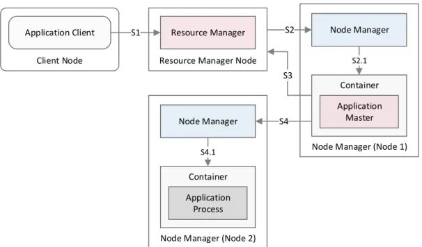
Figure 2.12. Application execution through YARN ... 25

Figure 2.13. Hadoop 2 + Tez stack... 26

Figure 2.14. Logical DAG... 27

Figure 2.15. Physical DAG showing the actual execution ... 28

Figure 2.16. Hive query execution architecture with Tez ... 30

Figure 2.17. Impala query execution architecture ... 32

Figure 2.18. IPTV high-level architecture ... 35

Figure 3.1. The Research Onion ... 38

Figure 4.1. Current data warehouse architecture... 46

Figure 4.2. Proposed data warehouse architecture... 47

Figure 4.3. Source file sample ... 50

Figure 4.4. Data preparation functional model ... 51

Figure 4.5. Data warehouse functional model ... 52

Figure 4.6.

Channel Tune

event transformation DFD... 56

Figure 4.7.

Program Watched

event transformation DFD ... 56

Figure 4.8.

DVR Events

transformation DFD ... 57

Figure 4.9.

Event Segmentation

example ... 57

Figure 4.10.

Event Segmentation

DFD ... 58

Figure 4.11.

Audiences Aggregation

DFD ... 58

Figure 4.12. RDBMS memory configuration ... 61

Figure 4.13. Staging Area tables physical model in the RDBMS ... 62

Figure 4.15. Fact tables physical model in the RDBMS ... 64

Figure 4.16. Aggregation tables physical model in the RDBMS ... 65

Figure 4.17. Ambari dashboard reporting the cluster overview ... 70

Figure 5.1.

Channel Tune

transformation benchmarking ... 75

Figure 5.2.

Program Watched

transformation benchmarking... 76

Figure 5.3.

DVR Events

transformation benchmarking ... 77

Figure 5.4.

Event Segmentation

benchmarking ... 78

Figure 5.5.

Audiences Aggregation

benchmarking ... 79

Figure 5.6.

Channel Tune

transformation scalability benchmarking ... 81

Figure 5.7.

Event Segmentation

scalability benchmarking ... 82

Figure 5.8.

Audiences Aggregation

scalability benchmarking ... 83

Figure 5.9. Storage usage comparison ... 84

Figure 5.10. Television

Channel Daily Overview

dashboard ... 86

Figure 6.1. Data transformation tasks cummulative execution time ... 88

Figure 6.2. Scalability effects on the data transformation tasks execution time ... 90

Figure 6.3. Total storage usage comparison ... 91

Figure 6.4. Enhanced data warehouse architecture integrating Hadoop ... 93

Figure 9.1.

Channel Tune

transformation execution plan... 158

Figure 9.2.

Program Watched

transformation execution plan ... 158

Figure 9.3.

DVR Events

transformation execution plan ... 159

Figure 9.4.

Event Segmentation

execution plan ... 160

Figure 9.5.

Audiences Aggregation

execution plan... 160

Figure 9.6.

Channel Tune

transformation DAG ... 186

Figure 9.7.

Program Watched

transformation DAG ... 186

Figure 9.8.

DVR Events

transformation DAG ... 187

Figure 9.9.

Event Segmentation

DAG ... 188

Figure 9.10.

Audiences Aggregation

DAG ... 188

Figure 9.11.

Intraday Television Share (%)

report ... 195

Figure 9.12.

Television Channel Reach (%)

report ... 196

Figure 9.13.

Daily Program Rating (%)

report ... 196

LIST OF TABLES

Table 1.1. Research objectives ... 3

Table 2.1. Example of data retrieval with SQL ... 10

Table 3.1. Research paradigms according to philosophical views ... 40

Table 3.2. Activity summary according to the Design Science steps ... 43

Table 3.3. Methodology summary ... 44

Table 4.1. Design and development activities ... 45

Table 4.2. Mediaroom event types ... 50

Table 4.3. Staging Area tables ... 53

Table 4.4. Inventory tables ... 54

Table 4.5. Support tables ... 54

Table 4.6. Fact tables ... 55

Table 4.7. Aggregation tables ... 55

Table 4.8. Color scheme for the data volume representation ... 55

Table 4.9. Hardware specifications of the host computer ... 59

Table 4.10. Data warehouse environment ... 60

Table 4.11. Tablespace configuration ... 61

Table 4.12. Implemented transformation processes ... 66

Table 4.13. Hadoop cluster environment ... 67

Table 4.14. Hadoop cluster service distribution ... 68

Table 5.1. Environment configuration for the performance tests ... 73

Table 5.2. Environment configuration for the scalability tests ... 81

Table 6.1. Comparison between RDBMS and Hadoop architectures ... 92

Table 9.1.

Channel Tune

event information ... 105

Table 9.2.

Box Power

event information ... 105

Table 9.3.

Trick State

event information ... 106

Table 9.4.

Program Watched

event information ... 106

Table 9.5.

DVR Start Recording

event information ... 107

Table 9.6.

DVR Abort Recording

event information ... 107

Table 9.7.

DVR Playback Recording

event information ... 107

Table 9.8.

DVR Schedule Recording

event information ... 108

Table 9.9.

DVR Delete Recording

event information ... 108

Table 9.10.

DVR Cancel Recording

event information ... 109

Table 9.11. SA_ACTIVITY_EVENTS table information ... 111

Table 9.13. SA_ASSET table information ... 113

Table 9.14. SA_CHANNEL_MAP table information ... 113

Table 9.15. SA_GROUP table information ... 113

Table 9.16. SA_PROGRAM table information ... 113

Table 9.17. SA_SERVICE table information ... 114

Table 9.18. SA_SERVICE_COLLECTION table information ... 114

Table 9.19. SA_SERVICE_COLLECTION_MAP table information ... 114

Table 9.20. SA_STB table information ... 114

Table 9.21. SA_SUBSCRIBER_GROUP_MAP table information ... 115

Table 9.22. SA_TV_CHANNEL table information ... 115

Table 9.23. SS_ASSET table information ... 115

Table 9.24. SS_CHANNEL_MAP table information ... 116

Table 9.25. SS_GROUP table information ... 116

Table 9.26. SS_MAP_CHANNEL_MAP_SERVICE table information ... 116

Table 9.27. SS_MAP_STB_CHANNEL_MAP table information ... 116

Table 9.28. SS_PROGRAM table information ... 116

Table 9.29. SS_SERVICE table information ... 117

Table 9.30. SS_SERVICE_COLLECTION table information ... 117

Table 9.31. SS_SERVICE_COLLECTION_MAP table information... 117

Table 9.32. SS_STB table information ... 118

Table 9.33. SS_STB_GROUP_MAP table information ... 118

Table 9.34. SS_SUBSCRIBER_GROUP_MAP table information ... 118

Table 9.35. SS_TV_CHANNEL table information ... 118

Table 9.36. LU_DATE table information ... 119

Table 9.37. LU_START_GP table information ... 119

Table 9.38. FACT_ACTIVITY_EVENTS table information ... 120

Table 9.39. FACT_ACTIVITY_EVENTS information mapping by event ... 121

Table 9.40. FACT_EVT_SEGMENTED table information ... 121

Table 9.41. AG_LIVE_RATING_DY table information ... 122

Table 9.42. AG_LIVE_REACH_DY table information ... 122

Table 9.43. AG_LIVE_SHARE_GP table information ... 122

Table 9.44. Oracle ‘write’ compression test

... 123

Table 9.45. Oracle 'read/write' compression test ... 123

Table 9.46. Hive 'write' compression test ... 161

Table 9.47. Hive 'read/write' compression test ... 161

Table 9.49.

Channel Tune

execution statistics in Hive ... 189

Table 9.50.

Program Watched

execution statistics in the RDBMS ... 190

Table 9.51.

Program Watched

execution statistics in Hive ... 190

Table 9.52.

DVR Events

transformation execution statistics in the RDBMS ... 190

Table 9.53.

DVR Events

transformation execution statistics in Hive ... 191

Table 9.54.

Event Segmentation

execution statistics in the RDBMS ... 191

Table 9.55.

Event Segmentation

execution statistics in Hive ... 191

Table 9.56.

Audiences Aggregation

execution statistics in the RDBMS ... 192

Table 9.57.

Audiences Aggregation

execution statistics in Hive ... 192

Table 9.58.

Channel Tune

execution statistics in Hive (scaled-out) ... 193

Table 9.59.

Event Segmentation

execution statistics in the RDBMS (scaled-up) ... 193

Table 9.60.

Event Segmentation

execution statistics in Hive (scaled-out) ... 194

Table 9.61.

Audiences Aggregation

execution statistics in the RDBMS (scaled-up) ... 194

Table 9.62.

Audiences Aggregation

execution statistics in Hive (scaled-out) ... 194

LIST OF ABBREVIATIONS AND ACRONYMS

1:1 One-to-One

1:M One-to-Many

3NF Third Normal Form

ACID Atomicity, Consistency, Isolation, Durability

AL Activity Logs

ANSI American National Standards Institute

BSS Business Support Systems

CBO Cost Based Optimizer

CPU Central Processing Unit

CRUD Create, Read, Update and Delete

DAG Directed Acyclic Graph

DB Database

DBMS Database Management System

DCL Data Control Language

DDL Data Definition Language

DFD Data Flow Diagram

DML Data Manipulation Language

DVR Digital Video Recording

DW Data Warehouse

EDW Enterprise Data Warehouse

ELT Extract-Load-Transform or Extraction-Loading-Transformation

EPG Electronic Program Guide

ETL Extract-Transform-Load or Extraction-Transformation-Loading

GB Gigabyte

GPON Gigabit Passive Optical Network

HDP Hortonworks Data Platform

HiveQL Hive Query Language

HPL/SQL Hybrid Procedural SQL

IP Internet Protocol

IPTV Internet Protocol Television

IS Information Systems

JDBC Java Database Connectivity

JVM Java Virtual Machine

LLAP Low Latency Analytical Processing

M:1 Many-to-One

MB Megabyte

MPP Massively Parallel Processing

MR Map-Reduce (in the context of Big Data) and Mediaroom (in the context of IPTV)

NoSQL Not Only Structured Query Language

ODBC Open Database Connectivity

ODS Operational Data Store

OLAP Online Analytical Processing

OLTP Online Transaction Processing

ORC Optimized Row Columnar

OSS Operational Support Systems

PGA Program Global Area

PiP Picture-in-Picture

PL/SQL Procedural Language/Structured Query Language

RCFile Record Columnar File

RDBMS Relational Database Management System

SA Staging Area

SQL Structured Query Language

STB Set-top Box

SVoD Subscription Video-on-Demand

TV Television

VoD Video-on-Demand

1.

INTRODUCTION

Big Data, infinite possibilities. The amount of information collected as of 2012 is astounding; around 2.5 Exabytes1 _{of data are created every day and this number is doubling every forty months (McAfee}

& Brynjolfsson, 2012). Like the physical universe, the digital universe is in constant expansion – by 2020 the amount of generated data annually will reach the 44 Zettabytes2_{, and by then we will have as many}

digital bits as stars in the universe (Dell EMC, 2014). Nowadays technologies under the umbrella of Big Data contribute decisively to the Analytics world (Henry & Venkatraman, 2015) and the availability of huge amounts of data opened the possibility for a myriad of different kinds of analyses that ultimately feed and enable decision support systems (Ziora, 2015). The ability to process these huge amounts of data, one of the key features of Big Data (Jin, Wah, Cheng, & Wang, 2015), is then of great interest to organizations as they acknowledge the benefits that can be extracted from Big Data Analytics (Kacfah Emani, Cullot, & Nicolle, 2015). Understanding then the importance of Big Data and its contribution to Analytics can be viewed under the simple concept that more is just better, since in data science having more data outperforms having better models (Lycett, 2013).

One source of large amounts of data is the Ericsson Mediaroom, a video platform that delivers Internet Protocol Television (IPTV) services to customers at their homes, like watching Live television or Video-on-Demand (Ericsson Mediaroom, 2016). Underneath this platform sits a Relational Database Management System (RDBMS) where millions of records are stored every day. These records reflect a variety of behaviors that can be performed by the television users at their homes, like changing a channel or a program. Periodically these events are sent to a centralized database and stored there. It is possible then to access them, in this centralized database, but for a limited time-window since the data is refreshed periodically due to volume constraints (Architecture of Microsoft Mediaroom, 2008). Therefore, if we want to store this data for future analyses, we need to extract it from this repository and store it in another location. From the extraction onwards, our research focuses on optimizing the processes surrounding the transformation of this raw data into valuable and actionable information. A comparative study is performed with the purpose of assessing the benefits of incorporating Big Data technologies in traditional data warehouse architectures, typically supported by an RDBMS. To achieve this, the required transformation processes are implemented in both the RDBMS and Hadoop, a software framework for storing and processing large data sets in a distributed environment of commodity hardware clusters (White, 2015).

This research explores the opportunities and challenges provided by the Big Data technological landscape and solves a specific problem that could not be previously solved by traditional relational databases due to the amount of information that needs to be processed.

1.1.

B

In traditional systems, when more processing capabilities are required, we are forced to expand their processing power by adding more and better resources, namely processors, memory or storage. This approach, known as vertical scalability, has associated high costs and it is constrained by the

architectural design that cannot evolve beyond the finite capabilities of one single node, the server (J. A. Lopez, 2012). In the Big Data world scalability is horizontal – instead of growing the capabilities of the individual servers, the Big Data infrastructure grows by simply adding more nodes to the cluster, the set of computers that work together in a distributed system (Ghemawat, Gobioff, & Leung, 2003). This scalability, when compared to the vertical scalability, offers infinite growing potential while the costs remain linear (Marz & Warren, 2015). Nowadays, due to the amount and speed of information generated from a multiplicity of sources, traditional Data Warehousing tools for data extraction, transformation and loading (ETL) are, in many cases, at the limit of their capabilities (Marz & Warren, 2015). Under these circumstances, the aim of this study is to explore and assess the value of Big Data technologies in the transformation of data, with the purpose of integrating them in traditional Data Warehousing architectures. The goal is not to replace data warehouses by Big Data infrastructures, but instead to put both worlds working together by harnessing the best features of each of them.

As the amount and types of available data have grown in the past years and will continue to grow, there is little doubt that the Big Data paradigm is here to stay (Abbasi, Sarker, & Chiang, 2016). The technologies that support the Big Data problems are relatively new, but their application, alongside traditional legacy Data Warehousing systems, presents itself as an interesting evolution opportunity. With both technologies working together, in a hybrid approach, we can offer the best of both worlds and apply them to warehousing architectures (Dijcks & Gubar, 2014; Russom, 2014).

Adoption of Big Data technology is a hot topic nowadays and the potential benefits are significant but, due to its young age, there are many challenges that need to be carefully addressed (Jagadish et al., 2014). Using Big Data as a transformation tool can be a solid first step in moving towards the world of infinite data. Hadoop’s ecosystem has several emerging data warehouse-style technologies that can be used to solve the problems that traditional technologies cannot overcome, when the volume and variety of data steps up (Kromer, 2014). When faced with huge amounts of data, how can traditional data warehouses evolve and maintain their value? This question poses the central topic on which this study is focused. In the end, managers need their questions answered and what is changing is the amount of information that is being used to support these answers (McAfee & Brynjolfsson, 2012).

1.2.

S

The main goal of this study is to assess and validate the feasibility of Hadoop as a data transformation tool that can be integrated as part of a traditional data warehouse. In other terms, our driving research question relates to the validation of the hypothesis stating that Hadoop can be used to augment traditional data warehouse architectures. To achieve this goal, Hadoop is used to calculate, from television viewing events, relevant television audience measurements like the Reach, number of individuals of the total population who viewed a given channel at any time across its time interval; Share, percentage of viewers of a given channel at a given time; and Rating, average population who viewed a program across its broadcasting time (Mytton, Diem, & Dam, 2016). These metrics are, ultimately, stored in a traditional data warehouse that corresponds to the single version of the truth in serving information to the decision support systems (Krishnan, 2013).

Big Data technologies, there is the necessity of designing and creating a Big Data Hadoop cluster. This lays the foundation for the study to implement the required processes and evaluate their results and performance.

It is also an objective of this study to assess the horizontal scalability potential that is offered by Hadoop clusters. The design of a solution for a problem should remain valid no matter the volume of data we intend to process. This is one of the greatest advantages of using Big Data technologies and in particular the Hadoop Distributed File System (HDFS) (White, 2015). When compared with traditional ETL technologies, Big Data technologies are able to scale seamless horizontally and adapt to big volumes of data (Kromer, 2014).

Table 1.1 briefly describes the six objectives that help to methodically reach the main goal of this research.

Objective

O.1 Investigate Hadoop’s state of the art and determine which solution is more appropriate for the problem at hand

O.2 Install a Hadoop cluster to serve as the foundation for the study

O.3 Make use of the selected Hadoop solution to transform Mediaroom’s raw data into meaningful television audience measurements, the Rating, Reach and Share

O.4 Measure and compare the performance of the implemented transformation processes in Hadoop against their performance in an RDBMS

O.5 Measure the processing scalability offered by the Big Data infrastructure and its corresponding performance improvements

O.6 Make the calculated audience measurements available through a visualization layer Table 1.1. Research objectives

1.3.

S

Besides exploring the general applicability of Hadoop as a transformation tool, and with that extend organizations’ current Data Warehousing capabilities, this study creates the procedures required to calculate television audience metrics from IPTV infrastructures like Ericsson’s Mediaroom. Nowadays, to collect audience measures we do not need to resort to population sampling anymore. Television service providers have all the data they need, what is missing are simply the right tools to convert this data into actionable knowledge. Thus, the importance of this study can be measured in two ways. On the one hand, it demonstrates how Hadoop can expand current data warehouse capabilities, and on the other hand, for television service providers, the study offers a tangible and scalable way of converting their current raw data into useful audience measurements.

1.4.

D

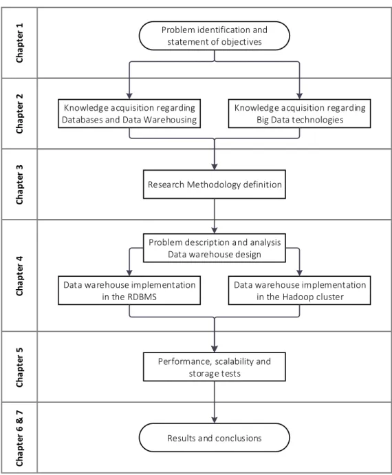
This dissertation follows the sequence of steps depicted in the diagram below.

C ha pt e r 2 C ha pt e r 2 C ha pt e r 1 C ha pt e r 1 C ha pt e r 3 C ha pt e r 3 C ha pt e r 4 C ha pt e r 4 C ha pt e r 5 C ha pt e r 5 C ha pt e r 6 & 7 C ha pt e r 6 & 7

Problem identification and statement of objectives

Knowledge acquisition regarding Databases and Data Warehousing

Knowledge acquisition regarding Big Data technologies

Research Methodology definition

Problem description and analysis Data warehouse design

Data warehouse implementation in the RDBMS

Data warehouse implementation in the Hadoop cluster

Performance, scalability and storage tests

Results and conclusions

2.

THEORETICAL FRAMEWORK

2.1.

I

The theoretical framework that supports this study crosses a wide-range of theories and techniques. Invariably, there is the need to go back to the origins of relational databases and from there expand the knowledge towards the focal point of the work, the current paradigms around the explosion of information under the umbrella of Big Data. There are many theories and emerging technologies that needed to be analyzed before we could start the implementation phase of this study.

Since the first ideas for the relational databases, proposed by Codd in 1970, the Relational Database Management Systems (RDBMS) have been the norm. With Codd’s ideas as a foundation, Online Transaction Processing (OLTP) systems proliferated within organizations; their features multiplied and their applicability allowed for a big dissemination and adoption in a wide range of Information Systems (IS). Relational databases, managed in OLTP systems, became the core of information in organizations, no matter their business purposes (Krishnan, 2013).

The myriad of applications that OLTP systems were supporting created a big divide in information inside organizations. The information was there, but the several systems did not communicate among themselves. With the purpose of creating a more systemic view of the organizations’ activities, the first concepts of Data Warehousing emerged in the late 1970s and early 1980s (Krishnan, 2013). The need for transforming data from many sources into useful insights paved the road for the importance of Business Intelligence and, for example, Enterprise Data Warehouses (EDW). Ralph Kimball is one the central figures in the world of data warehouses and in particular in the definition of the dimensional modeling, a variation of the traditional relational model, and the basis of data warehouses’ design (Kimball & Ross, 2013).

Within the world of data warehouses and Business Intelligence, there are several techniques for the purpose of providing valuable insights that can be explored through the transformation of data into, ultimately, actionable knowledge. Making use of the dimensional modeling defined by Kimball, the Online Analytical Processing (OLAP) is an extremely useful approach for delivering fast answers from different perspectives (Codd, Codd, & Salley, 1993). Business Intelligence and Analytics have relied, for many years, on the dimensional models and online analytical processing tools that enable the exploration of business information. The standard approaches, that are associated with data warehouse systems, are still very much alive and proof of that is that 80–90% of the deliverables in Business Intelligence initiatives are supported by OLAP built upon an RDBMS-based data warehouse (Russom, 2014).

barriers of Codd’s relational model were created and as a result, the NoSQL (Not only SQL3_{) paradigm}

gained popularity and momentum. NoSQL options, when compared with the traditional RDBMSs, are very simple in their sophistication levels. RDBMSs evolved through decades and these new approaches, in a technological view, look like a return to the past (Mohan, 2013). Traditional RBDMSs are also evolving to allow horizontal scalability while maintaining the integrity of a dimensional database. The Massively Parallel Processing (MPP) paradigm can be seen as a response, by the traditional RDBMSs, to the vast amounts of data and it represents an important approach in the Big Data world (Stonebraker et al., 2010).

The purpose of data warehouses and Big Data, within organizations, is seen through different eyes by several authors. While data warehouses provide a source of clearly defined and unified information that can then be used by other systems like Business Intelligence tools (Kimball & Ross, 2013), some authors state that purpose of Big Data is to provide cheap solutions to store raw data that hasn’t any predefined structure (Boulekrouche, Jabeur, & Alimazighi, 2015). This idea is even emphasized by authors advocating that there is no correlation between data warehouses and Big Data, since the latter is only seen as a technology for storing data (B. Inmon, 2013). Moreover, in the opposite side, some defend that Big Data itself consists of both technologies and architectures (Maria, Florea, Diaconita, & Bologa, 2015). The Data Warehousing Institute strongly believes that Hadoop cannot replace a traditional data warehouse since, for example, enterprise data reporting requirements cannot be satisfied by Hadoop as well as they can be by an RDBMS-based data warehouse. Technologies have completely different levels of maturity, and in the end, the most important aspect is which approach can better suit the specific objectives (Russom, 2014).

Hadoop can be seen as the next step in the development of data warehouses and especially in the Extract-Transform-Load (ETL) phase, even though Hadoop is not an ETL tool (Šubić, Poščić, & Jakšić, 2015). Combining new technology as an integrator of data in a traditional data warehouse is explored so that its advantages and shortcomings can be assessed in an empirical way that goes beyond the theory and the so many contradictory opinions in the world of data science.

2.2.

R

When we speak about relational databases it is mandatory to go back to 1969-1970 and more specifically to the seminal publications “Derivability, Redundancy and Consistency of Relations Stored in Large Data Banks” (Codd, 1969) and “A Relational Model of Data for Large Shared Data Banks” (Codd, 1970) by Edgar Frank Codd. Codd’s second publication is the single most important event in the history of databases and its proposed relational model is still a part of the vast majority of databases (Date, 2003). The relational model appears as a response to the challenges of managing a growing amount of data. It is primarily focused on the independence between data and applications, and with the problems of inconsistency typically associated to data redundancy.

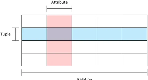
Within Codd’s proposal, for the original relational model, we can discern three major components – structure, integrity and manipulation (Date, 2015). As structure features, firstly we have the relations that are commonly referred as tables. These relations contain tuples that can be interpreted as the

rows of a table, and finally, a tuple is constituted by a set of attributes that instantiate values from the valid domains (also referred as types).

Relation Attribute

Tuple

Figure 2.1. Visual representation of a Relation, Tuple and Attribute

In Figure 2.1 we have a visual representation of a relation with a set of tuples containing each five attributes. This relation can also be expressed as a table containing multiple rows, each with five columns. In the depicted example, we are considering a five-ary relation since the number of attributes (or columns) is used to express the arity of the relation. Attributes inside relations contain actual values within their corresponding domain. As an example, an attribute expressing European countries could only contain values belonging to the conceptual pool of European countries.

Still, regarding the structure of the relational model, we have to consider several kinds of keys. Relations need to have at least one candidate key capable of expressing the uniqueness of a tuple. These keys can be composed of one or more attributes. What is required is that the relation has a unique key value for each distinct tuple. From the candidate keys, we can elect one to be the primary key and thus being subject to special treatment. Finally, we have the foreign key that is defined by one or more attributes in a given relation R2 that must also exist as a key K in some other relation R1.

When we approach the aspects of the model structure, that emphasize the importance of data consistency, it is important to mention data normalization and the normal forms. The goal of data normalization is to reduce or even eliminate data redundancy. That is expressed in the model definition by splitting relations, with redundant information, into two or more relations. Even though relational theory defines several normal forms, the one most commonly used in relational models is the Third Normal Form (3NF) since it covers most of the anomalies related to the update of redundant data (Sumathi & Esakkirajan, 2007). The 3NF builds upon the two previous normal forms and states the following:

1. All attributes contain only atomic values (First Normal Form);

2. Every non-key attribute is fully dependent on the primary key (Second Normal Form);

3. Every attribute, not belonging to a candidate key, is non-transitively4 _{dependent on every key.}

The integrity features, from the relational model main components, allow us to enforce rules in the model, with the purpose of assuring consistency in the data and in the relationships that help shape and express the logical concepts into the relational model. Simply put, the original relational model bases its integrity features in two generic constraints, one related to the primary keys and another related to the foreign keys. The entity integrity rule states that primary keys should represent uniquely the tuples and for that purpose they cannot contain null values, and the referential integrity rule establishes that there cannot be any unmatched foreign key values in the corresponding target candidate key. A more implicit constraint can also be considered, the attribute integrity that states that an attribute value must belong to its specified domain.

The manipulative features enable us to query and update the data stored in the model. They relate to relational algebra and relational algebra assignment which allow us to assign the value of a given relational algebra calculation to another relation (e.g., R3 = R1 INTERSECT R2). In relational algebra, we can identify the following original operators:

• Restrict– returns a relation filtered by a given expression; • Project – defines the attributes that will be part of the relation;

• Product– returns a relation containing all the possible tuples resulting from the combination of two tuples belonging to two different relations. This operator is also known as cartesian product/join;

• Union – returns a relation containing the tuples that exist in any of two given relations; • Intersect – returns a relation containing the tuples that exist in both the specified relations; • Difference – returns a relation containing the tuples that exist in the first relation but not in

the second;

• Join – originally named natural join; it returns the tuples that are a combination of two tuples from two distinct relations that share the same values in the common attributes.

The relational model itself, as published by Codd, does not establish a formal language per se to implement these operators and enable the described manipulative features. That role was taken afterward by SQL (Structured Query Language).

2.3.

S

Q

L

SQL was originally developed by IBM, under the name of Structured English Query Language, with the purpose of manipulating and retrieving data stored in Codd’s relational model. Its first commercial implementation was released in 1979 by the company that is nowadays Oracle (Oracle Corporation, 2016). Even though SQL’s design foundation was Codd’s relational model, it deviates in some ways from its original definitions. In SQL, for example, we can apply order to the data retrieval, and tables are viewed as a list of rows instead of a set of tuples. On this spectrum, we can find criticism arguing that SQL should be replaced by a language strictly based on the original relational theory (Darwen & Date, 1995).

RDBMSs commonly also include procedural languages that extend SQL features like Oracle’s PL/SQL (Procedural Language/Structured Query Language) or Microsoft’s Transact-SQL. As mentioned, SQL is indeed standard for relational databases, but despite this, many RDBMSs vendors do not follow strictly the standard convention, currently the SQL:2011, and implement their own variations. However, the ANSI5 _{SQL standard is supported in most major RDBMSs, thus making SQL interoperability a great asset}

that contributed to its adoption.

SQL’s vendor independence based on official standards and associated to a high-level, English-like language, are some of the aspects that contributed to SQL’s success (Weinberg, Groff, & Oppel, 2010). This complete and common language for all relational databases also assures that the developers’ skills remain valid when moving from one vendor to another since all programs written in SQL are portable and require little or no modification for them be moved from one RDBMS to another (Oracle Corporation, 2016).

As stated, SQL enables its users to retrieve and manipulate data stored in relational databases. For that purpose, SQL has a set of predefined commands that can be divided, according to their scope, in three types – the Data Manipulation Language (DML), the Data Definition Language (DDL), and finally the Data Control Language (DCL), that according to ANSI SQL is considered to be a part of the DDL.

SQL SQL

DDL DDL DML

DML DCLDCL

CREATE ALTER

DROP INSERT

SELECT UPDATE

DELETE

GRANT REVOKE

Figure 2.2. SQL's three types of commands

From the figure above we can discern SQL’s three types of commands. DML implements the four basic functions of persistent storage – create, read, update and delete (CRUD) (Martin, 1983). DDL is used to create, alter or drop objects like tables, views, constraints or indexes. Moreover, the DCL commands allow us to control access to the database objects by granting or revoking permissions to users.

SQL is much more than a query language as its name suggests. Querying data is one of the most important functions performed by SQL but it is not the only one. It enables the users to control many aspects of a Database Management System like:

• Data retrieval – through SQL users can query the database and retrieve the desired information. One example of data retrieval statement is presented on Table 2.1;

• Data manipulation – applications or users can add new data and update or delete previously stored data;

• Data sharing– SQL is also used in the coordination of concurrent accesses by assuring ACID6

properties in the transactions (Haerder & Reuter, 1983);

• Data definition– SQL lets the users define the structure and the relationships of the model responsible for storing the data;

• Data integrity – to avoid data inconsistency SQL allows for the definition of constraints that assure data integrity;

• Access control – SQL can be used to protect data against unauthorized access. Through the Data Control Language, it is possible to restrict the users’ ability to retrieve, add, modify or delete data.

SQL Statement Operator Description

SELECT t1.column1, t2.column3 PROJECT Defining the data retrieval projection FROM table1t1 Source Retrieving data from a given table JOIN table2t2

ON (t1.column1 = t2.column1) JOIN Performing a join with a second table WHERE t1.column2 >= value RESTRICT Restricting the output by a given criteria ORDER BY t1.column1 ASC Order Specifying the result order

Table 2.1. Example of data retrieval with SQL

In Table 2.1 we can see an example of a SQL query that will retrieve data from the data model. In the column ‘SQL Statement’ the language keywords are highlighted, and in the column ‘Operator’ we can observe, also highlighted, the original operators from relational algebra. Note the use of aliases when referring to the tables to simplify references to their columns (e.g.: table1 has the alias t1).

SQL databases are extremely powerful as they enable the combination and analysis of data through the simplicity of relational algebra. They can be used to represent a single point in time and a single point in space through their transactional serializability and their clear context isolation, respectively. As a language, SQL allows the developers to easily express their intent and navigate the relational model effectively and efficiently (Helland, 2016).

2.4.

R

D

M

S

We can define a database as an organized and interrelated collection of data, modeled to represent a specific view of reality, and a Database Management System (DBMS) as a complex system with the purpose of managing databases (Date, 2003). The DBMS essentially manages three aspects: the database schema that defines the data structure, the data itself and the database engine that enables the interface between the users and the data.

The categorization of a DBMS can be done by its underlying implementation model, and therefore we can simply just say that a Relational Database Management System is a DBMS that manages a relational database and, in most cases, uses SQL. This is a simplistic view since to correctly classify a DBMS as relational it must adhere to “Codd’s 12 rules” (Codd, 1985).

One of the objectives of a DBMS is data availability and, to that end, it acts as an interface between the users and the data by translating the physical aspects, involved in storing and organizing the data, into a logical view that can be easily accessed by users and applications. The DBMS is also responsible for the correctness of the data it stores, and thus data integrity is a fundamental objective present in these management systems. When providing data to the users, a DBMS needs to have a set of functionalities with the purpose of assuring that only authorized users can retrieve and manipulate the data they are intended to and this takes us to another objective of a DBMS, data security. Finally, a DBMS also provides an abstraction layer of how data is stored inside the database, through the use of complex internal structures, specifically concerned with storage efficiency. This is data independence and allows for the users to store, manipulate and retrieve data efficiently (Sumathi & Esakkirajan, 2007).

Database management systems provide several benefits that empower users in their data management activities. Users understand the logical view of data without having to concern with the complex physical mechanisms that work to assure that the correct data is available in the most efficient way. DBMSs provide a centralized data management entity where all the data and related files are integrated in one single system. With this, data redundancy is minimized while, at the same time, its consistency and integrity can be more effectively assured. DBMSs also play an important part in application architecture since they enable independence between applications and data.

When we speak about Database Management Systems we are abstracting ourselves from the underlying model present in their database engine, but, in most cases, we are implying that we are dealing with the relational model and, therefore, the DBMS is an RDBMS. This is true because even though there are many approaches to the data model, it is the relational model that is effectively the most important one from both theoretical and economic perspectives (Date, 2003).

2.5.

D

W

The benefits provided by DBMSs made data a more accessible asset and enabled the creation of effective applications and systems throughout organizations with the purpose of supporting their specific processes. These systems were initially individual entities that managed their information and this led to an uncontrolled proliferation of data. Organizations had in fact data about their activities, but it was hard to find it and even harder to assert if it was correct. The existence of a multitude of departmental truths, solely based on isolated views, made the task of finding the single organizational version of the truth very difficult (W. H. Inmon, 2005). This need for an organization-wide single version of the truth, which could be easily used by the decision support systems, triggered a paradigm shift in information architecture that consequently gave origin to the concept of Data Warehousing (W. H. Inmon, Strauss, & Neushloss, 2008).

from transactional operational systems, transforming it into meaningful information so that it can be easily accessed by the users in order to promote data analysis and enable fact-based business decisions (Kimball & Caserta, 2004).

Data warehouses and their architectures vary according to the specific realities and requirements of each organization. We can find multiple architectures and also different design approaches when it comes to building a DW (Sumathi & Esakkirajan, 2007). In Figure 2.3 we present a high-level architecture for a data warehouse designed with the top-down approach. This approach consists of firstly creating the data warehouse itself, with an enterprise-wide vision, and then expanding it by adding data marts with more subject-oriented views. The top-down approach provides consistent dimensional views across all data marts since they are generated from the data warehouse and not from the operational systems. This centralized approach is also robust when it comes to business changes since the implementation of data marts only depends on the data warehouse. However, designing a full data warehouse requires considerably more effort, and thus costs, when we compare it to the implementation of single data mart from an operational system as it is proposed by the bottom-up approach. With the bottom-up approach it is possible to deliver faster results since implementing single data marts, as the requirements evolve, requires lower initial investments than creating the full enterprise-wide data warehouse. The data warehouse is then built from the information in the data marts (Imhoff, Galemmo, & Geiger, 2003; Sen & Sinha, 2005). Both approaches have their advantages, and it is possible to use them together in a hybrid approach that combines the development speed and the user-orientation of the bottom-up approach with the enterprise-wide integration enforced by the top-down approach (Kimball & Ross, 2013).

Database X

Files

Web Source

Database Y

Data Mart I

OLAP Cube II OLAP Cube I

Data Mart II Metadata

Summary Data

Detailed Data Data Warehouse

Figure 2.3. Data warehouse architecture with data marts

the Data Access and Analysis tier that is composed by a set of tools that make use of the data, ranging from simple descriptive analytics, like reporting, to predictive analytics that can, for example, include data mining. We could also easily split the data warehouse and data marts tier into two different tiers, one related only to data storage that would include the data warehouse and the data marts and another tier specifically dedicated to analytics that would contain for example the OLAP cubes. Nevertheless, in all Data Warehousing architectures, we can identify a layer that represents the data sources, presented in Figure 2.3 as the Operational Systems. The data sources themselves are not part of the data warehouse architecture per se, even though they are critical to its design, but they rather represent the source of all data that can originate from any system throughout the organization and even from external entities. Therefore, we have considered, as the first tier of the data warehouse architecture, the ETL.

2.5.1.

ETL/ELT

The Extraction-Transformation-Loading layer is the foundation of a data warehouse. It is responsible for extracting data from different operational systems and combining it in a way that makes possible to use it together, while at the same time assuring its consistency and quality. Moreover, the role of the ETL is to make this transformed data available for the applications associated to data analysis and decision making. The ETL tier is hidden from the users but its processes, within the DW architecture, are the ones that require more resources for their implementation and maintenance (Kimball & Caserta, 2004).

ETL is far more than just getting data from the sources and deliver it to the users. It can contain complex processes with the purpose of cleaning and conforming heterogeneous sources into a single and unified enterprise-wide view of the captured systems. This flow of data can be achieved by different ETL architectures that can be put into place to better fit the transformation requirements. For example, it is common to find a Staging Area within the ETL tier. This area is where the extracted data is placed and subsequently undergoes successive transformations before it can be loaded into the data warehouse. The need for a Staging Area is more or less related to the data quality in the sources and the complexity around their transformation and combination (Malinowski & Zimányi, 2007).

Some early DW architectures also contained an Operational Data Store (ODS) that could be seen as an extension of the ETL layer. The ODS is a hybrid construct that seats between the operational and the decision-support systems. Its purpose is to provide low-latency reporting capabilities that could not be obtained from the DW due to its slower refresh periodicity. Nowadays the use of dedicated ODS is not very frequent and their role was absorbed by the DW itself (Kimball & Caserta, 2004).

the inclusion of new data sources and it is more adaptable to business requirements changes. The data is loaded in its raw format, and, therefore, multiple transformations can be applied as the requirements change. ELT addresses some of the inflexibility of ETL when it comes to environmental changes as it brings data closer to the users and speeds up the implementation process (Marín-Ortega, Dmitriyev, Abilov, & Gómez, 2014).

In recent years, the diversification of DW workloads is leading to distributed architectures where, for example, the ETL processes are being offloaded from expensive dedicated platforms to cheaper solutions like Hadoop (Clegg, 2015). Hadoop can be seen as the next step in the design and implementation of data warehouses, with special emphasis in the ETL layer (Šubić et al., 2015). We approach this hybrid architecture that brings Big Data technologies into the data warehouse ecosystem in section 2.8.

2.5.2.

Dimensional modeling

When it comes to designing data warehouses, we cannot escape the discussion around Inmon’s top -down approach, supported by operational data in the third normal form, and Kimball’s bottom-up approach supported by data marts implemented with dimensional models (Breslin, 2004). Both approaches have their differences, as presented previously, but they can be combined in the implementation of data warehouses so that we can benefit from the merits found in each one (W. H. Inmon et al., 2008).

Kimball’s dimensional modeling, published in the first edition of “The Data Warehouse Toolkit”, became the leading design technique to implement data warehouse models (Kimball & Ross, 2013). The dimensional model is especially oriented to the delivery of data for analysis with emphasis in performance. We can qualify its main benefits, when compared to entity-relationship models, as being a model that facilitates understandability and enables performance by using a less normalized data model. Data normalization, like the third normal form, is critical to assure data integrity but it has the negative effect of making more difficult to interpret the models and the information they support and, at the same time, it hinders data access performance. Redundancy harms integrity, but it helps performance and understandability. Another benefit, also related to the simplicity of the model, is the extensibility that it adds to the design. Due to the simple structure of the model, it is a lot easier to adapt it to new requirements. Adding new concepts to a normalized model requires a great deal of more effort to assure its full consistency, while in a dimensional model it can be achieved by just adding more rows to represent a fact or more columns to identify a dimension (Kimball & Ross, 2013). Extensibility is then easier to implement but, at the same time, it is limited up to a certain degree due to the dependence of the model regarding the initial requirements (W. H. Inmon et al., 2008).

Figure 2.4. Star schema diagram

In the star schema design, shown in Figure 2.4, the model is not in the 3NF, but instead it is denormalized. The process of denormalization consists in reducing the normalization of a given model into a less normalized form, e.g. starting from a model in the 3NF, denormalization can produce a new model in the second or even first normal form. The process of denormalization grants performance benefits to data retrieval since it can eliminate joins that otherwise would be necessary to navigate the model but, on the other hand, a denormalized model requires a more complex update process to ensure data consistency because it adds redundancy.

Figure 2.5. Snowflake schema diagram

purpose of eliminating redundancy, the dimension tables are normalized, usually in the 3NF, and can be connected to each other through many-to-one relationships.

Choosing between the star schema and the snowflake schema is a balance between complexity, performance, and consistency, where business requirements and the technological infrastructure should also be considered. We can also find other designs like the starflake, where we can find both normalized and denormalized dimensions and also the constellation schema that consists of multiple fact tables that share the same dimension tables (Malinowski & Zimányi, 2007).

2.5.3.

DW 2.0

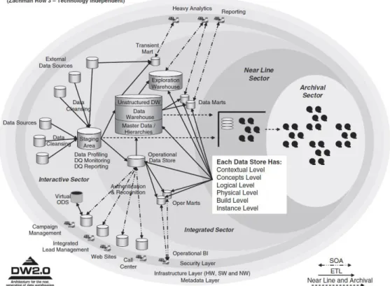
As businesses and technology evolve, so do IS architectures. The DW 2.0 architecture is the product of evolution amongst established architectures, namely the ones proposed by Inmon and by Kimball. The DW 2.0 paradigm fits together the corporate information factory concept, which advocates the data warehouse as the single version of the truth, with Kimball’s architecture centered in data marts. Its focus relates to the basic types of data (structured and unstructured), their supporting structure and how they can relate, in order to establish a central data store capable of satisfying organizations’ informational needs and enabling their decision support systems (W. H. Inmon et al., 2008).

The DW 2.0 architecture incorporates several aspects surrounding the diversity of data. Both structured and unstructured data are considered as essential, and the recognition of the lifecycle of data plays a determinant role within this architecture. Also, at the heart of the architecture, metadata is deemed as an essential component containing both technical and business definitions. Metadata in the DW 2.0 represents a cohesive enterprise view capable of capturing and coordinating all sources of metadata distributed across the organization.