UNIVERSIDADE FEDERAL DE MINAS GERAIS INSTITUTO DE CIˆENCIAS EXATAS
PROGRAMA DE P ´OS-GRADUA ¸C ˜AO EM ESTAT´ISTICA
A Bayesian Skew Mixture Item Response Model
Juliane Venturelli
Orientador: Fl´avio Bambirra Gon¸calves
Co-Orientadora: Rosangela Helena Loschi
Abstract
Under the Item Response Theory, the two most common link functions used to model
dichoto-mous data are the symmetric probit and logit. However, some authors have emphasized that
these symmetric links do not always provide the best fit for some data sets. To overcome this
issue, asymmetric links have been proposed. This work aims at introducing a flexible Item
Response Model able to accommodate both symmetric and asymmetric link. The c.d.f. of a
centered skew normal distribution is assumed as the link function and, additionally, we
con-sider a finite mixture of Beta distributions and a point mass distribution at zero to describe
the uncertainty about the skewness parameter, so not all items need to be assumed asymmetric
a priori. Therefore, the proposed model embraces symmetric and asymmetric normal models in one also performing an intrinsic model selection. We offer the full condition distribution
of ability, discrimination and difficulty parameters. We also introduce efficient algorithms to
`
Agradecimentos
Vocˆe sabe por que como ra´ızes? Porque ra´ızes s˜ao importantes 1.
Sou muito grata pela constante ajuda, suporte e orienta¸c˜ao do Professor Fl´avio Bambirra,
um dos professores de conhecimento mais vers´atil que conheci na Estat´ıstica, de ideias geniosas
e ousadas. Tenho certeza de que em poucos anos seu nome estar´a no hall dos estat´ısticos
de destaque. Sou muito grata `a Professora Rosangela Loschi, que aceitou o desafio de me
co-orientar em TRI. Muito obrigada por deixar meu trabalho mais colorido!
Sou imensamente grata ao papy e `a mamy, que n˜ao mediram esfor¸cos para investir em
minha educa¸c˜ao acadˆemica. Especialmente, agrade¸co meu pai por sempre se dispor a me
ajudar com o meu “software”. Mais ainda, agrade¸co por serem exemplos de esfor¸co e dedica¸c˜ao.
Definitivamente n˜ao sei como meu pai conseguiu fazer Engenharia e minha m˜ae Medicina, tendo
que trabalhar e ainda com trˆes filhas...!
Minha sincera gratid˜ao ao Br´aulio pela indescrit´ıvel disposi¸c˜ao em me ajudar nos
proble-mas mais diversos. Agrade¸co `a Larissa, aluna destaque do mestrado, L´ıvia, sempre neutra, e
Rachel, com quem n˜ao tem como discutir, pela presen¸ca no caf´e, no bandej˜ao, nos choros, e
por aguentarem minhas rabugentices. Agrade¸co `a Gabi por sempre oferecer ajuda, e `a Raquel
Borges pelas ajudas com o ggplot. Agrade¸co `a minha querida amiga Marina Flor Muniz, por quem eu tenho enorme admira¸c˜ao n˜ao s´o pela excelˆencia acadˆemica, mas por conseguir viver
fora do aqu´ario. Sou muito grata pela minha amizade com Vivi Paix˜ao, quem conheci na luta,
e que viveu comigo os mesmos dramas e desesperos de uma aluna de mestrado. Agrade¸co `a
Bruna, pelo constante apoio, carinho e compreens˜ao, `a Esther pelas “caronas”; ao Jaider -que
n˜ao ajudou em nada!-, e `a Tamires pelos ensaios sobre as ilus˜oes da Ciˆencia. Agrade¸co ao
Gustavo Souza por ter parado suas balb´urdias quˆanticas para (tentar) me ensinar An´alise.
Agrade¸co `a Lay pelas muitas amostras gr´atis e muitos acolhimentos. Agrade¸co `a Let´ıcia
Malta, talvez a pessoa de maior inteligˆencia interpessoal que j´a conheci, a quem sou eternamente
grata por me ajudar a ser mais leve, centrada e forte. Ao Bup, que nesses dias de conclus˜ao de
trabalho me colocou para cima.
Agrade¸co `a Bruna e Carol, simplesmente por estarem sempre l´a, ainda que longe.
Agrade¸co `a V´o Nice, `a V´o Irene e aos avˆos Ol´ıvio e Abelardo (ainda que n˜ao os tenha
Acknowledgement
The authors would like to thank all of the people who contributed in some way to the work
described in this dissertation.
This work was accomplished with the help and support of fellow lab-mates and collaborators.
We would like to especially thank Br´aulio Veloso and Professor Marcos Prates for being very
helpful in finding a clever solution to a numerical problem, which had cost us considerable
time and headache. We would like to thank Douglas Mesquita and Luis Gustavo Silva for
their constant contributions in troubleshooting in R and Latex. We also would like thank the
contributions of Professor Dani Gamerman, and James Olson for the English support.
Contents
1 Skew Distributions with Normal Kernels 12
1.1 Skew Normal Distribution . . . 12
1.2 Centered Skew Normal Distribution . . . 16
1.3 A General Class of Multivariate skew Normal Distributions . . . 20
2 Binary Item Response Models 22 2.1 Symmetric IRM . . . 23
2.1.1 The Rasch Model . . . 23
2.1.2 Two-Parameter Models . . . 25
2.1.3 Three-Parameter Models . . . 26
2.2 Skew IRM . . . 28
2.2.1 Skew Logit Model . . . 28
2.2.2 BBB Skew Probit Model . . . 30
2.2.3 Skew Normal model IRT under the Centered Parametrization . . . 31
3 A Flexible Class of Centered Skew Probit IRT Model 33 3.1 Proposed Model . . . 34
3.2 Prior Specifications . . . 35
3.3 Posterior Distribution . . . 37
3.4 MCMC . . . 37
3.4.1 Full Conditional Distribution for X . . . 39
3.4.3 Full Conditional Distribution for (a, b) . . . 41
3.4.4 Full Conditional Distribution for p . . . 44
3.5 Full Conditional Distribution for Z . . . 45
3.6 Full Conditional Distribution for γ− and γ+ . . . 46
3.7 Computational Aspects . . . 47
3.7.1 Sampling of X . . . 47
3.7.2 Sampling of θ and (a, b) . . . 48
3.7.3 Sampling of Z . . . 49
4 Simulations 51 5 Final Remarks 56 5.1 Full Conditional Distribution for θ . . . 57
5.2 Full Conditional Distribution for (a, b) . . . 59
Introduction
Item Response Theory (IRT) is a psychometric theory commonly used in educational
assess-ments and cognitive psychology. It aims to model variables which are by nature unobservable,
such as abilities, intelligence and depression. As these variables are constructs rather than
physical attributes, they are often called latent traits. Although these traits are not directly
measured, an individual’s responses to a test provide information from which traits can be
inferred. In this work, the terms “ability”, “latent traits”, or simply “traits”, are going to be
used indiscriminately with the same meaning. As our focus is on the use of IRT in the
educa-tion field, the main interest is to model the relaeduca-tionship between responses and abilities of J
individuals submitted to a test comprised by I items.
Under the latent theory, it is customary to assume that only one trait influences, or
deter-mines, a person’s performance when taking a test. Although this assumption is not reasonable
in practice, it is enough to assume that a dominant factor influences on a test performance. This
dominant factor is referred to as the ability measured by the item. Models that consider only
one ability are called unidimensional models. However, more complex models are available to
take into account a multidimensional vector of abilities (Van Der Linden & Hambleton, 1997).
In IRT, models are built taking into account that the relationship between an examinee’s2
item performance and the dominant trait is described by a monotonically increasing function
denominated item characteristic curves (ICC). The choice of the ICC and its parameters is a
crucial part of IRT. The well known item response models (IRM) for dichotomous responses,
for instance, adjust response data for item characteristics such as difficulty, discriminating
power and liability to guessing. Some most well known IRM’s are presented and discussed in
Chapter 2.
Early work in the IRT field was first addressed in the works of Richardson (1936), Lawley
(1943) and Tucker (1946). However, most contemporary concepts of IRT were formulated
around the 1950s and 1960s, mainly by Lord (1952), Rasch (1960), Birnbaum (1957, 1958),
Lazarsfeld & Henry (1968) and Wright & Panchapakesan (1969). Also, a major contribution
to IRT was given by Samejima (1969, 1972) who introduced a new IRM able to handle both
polychotomous and continuous response data. Samejima (1972) also extended unidimensional
models to the multidimensional ones.
A startup and yet revealing work on IRT can be found in the book by Baker (2001) entitled
The Basics of Item Response Theory. In Portuguese, the reader can resort to de Andrade et al. (2000) for a brief and comprehensive work on basic concepts. Some more detailed work
can be found in Baker (1977), who provided a comprehensive review of parameter estimation
methods. Van Der Linden & Hambleton (1997) offered a book with a collecting of complex
IRM, such as models for multiple abilities or cognitive components and nonmonotone items, and
nonparametric models. Also, some important estimation methods (EM and Bayesian approach)
for dichotomous and polichotomous items were discussed by Azevedo (2003), and for a more
complete work on the Bayesian approach to modern test theory, the reader can resort to the
book by Fox (2010).
A common assumption in modelling academic ability and other latent traits associated with
human behaviour is to assume that these traits follow a standard normal distribution. Such
an assumption asserts that one believes the abilities population has a normal shape, and the J
students taking the test are a random sample of this population. However, this assumption is
not always observed in psychometric data, as noticed by Micceri (1989). Samejima (1997) also
questioned the indiscriminate use of normality assumption without even checking its adequacy,
and Azevedo et al. (2012) showed data sets where normality and symmetry did not entirely hold.
To overcome this issue and to obtain better estimations for traits, some flexible approaches have
been considered. Mislevy (1984), for instance, considered a mixture of normal distributions and
a nonparametric estimation based on empirical histograms. Bazan (2005) proposed a flexible
item response model by using the skew normal distribution (SN) (Azzalini, 1985) to model
the behaviour of the ability parameter. However, according to Azevedo et al. (2011), Bazan
(2005) did not consider the estimation of the skewness parameter concomitantly with the model
estimation, neither addressed issues concerning to the model identifiability. To overcome the
identifiability problem, Azevedo et al. (2011) considered the Centered Skew Normal distribution
advantages to the model inference and the estimation of item’s parameters. A brief presentation
of the SN and CSN families of distributions is given in Chapter 1.
Another common feature of IRT is the usage of symmetric probit and logit link functions
for ICC. However, it has been emphasized by some authors that these symmetric ICCs are not
always appropriate for describing the relationship between examinee’s ability and the
proba-bility of success (correct answer). According to Chen et al. (2000), the commonly used links
for binary response data do not always fit the dataset properly, which can lead to biased
esti-mation of the model parameters. Many authors have proposed possible solutions to overcome
this issue. For instance, Samejima (2000) proposed a family of models, the so called Logistic
Positive Exponent Family, which provides asymmetric ICCs and has the logistic model as a
special case. In this class of models, the ICC is given by L(·)ǫi , where L(·) is the cumulative
distribution function (c.d.f.) of the standard logistic distribution, and ǫi > 0 is the skewness
parameter associated with the ith item. The logistic link is recovered when ǫ
i = 1. Santos
(2009) presented an extension of the proposed model by Samejima (2000), allowing the
guess-ing parameter to be different from zero, and usguess-ing a prior specification to detect asymmetric
items. For the skewness parameter ǫ, Santos (2009) considered a finite mixture type
distribu-tion with a point mass at one. Addidistribu-tionally, another asymmetric link funcdistribu-tion was obtained
by Baz´an et al. (2006), who considered the Skew Normal (SN) distribution (Azzalini, 1985) to
model the ICC, thus, obtaining an asymmetric IRM that admits asymmetric items. Since the
SN distribution has the normal one as a special case, the probit IRT model is included in the
skew probit class of IRMs. These models are briefly reviewed in Section 2.2.
In this work, we focus on dichotomous unidimensional IRMs and inference is made under
the Bayesian approach. Our main interest is to build a flexible IRT model able to
accommo-date both symmetric and asymmetric ICC. Differently from what is presented in Baz´an et al.
(2006), we introduce a skewed ICC based on the CSN distribution. One of the most important
contributions of this work is to consider a finite mixture of Beta distributions and a point mass
at zero to describe the uncertainty about the skewness parameter. Therefore, the proposed
model embraces both probit and skew probit models which, under our approach, have a non
methodology for model selection. We offer the full condition distribution of ability,
discrimina-tion and difficulty parameters. We also propose efficient algorithms, based on Markov Chain
Monte Carlo (MCMC) methods, to sample from the posterior distribution.
In regard to its structure, this work is organized as follows. In Chapter 1 we review the SN
and the CSN families of distribution (Azzalini, 1985) and some of their properties, since skewed
distributions with normal kernels play an important role in our approach. We also review
and make some adaptations for the family of distribution with Normal kernel introduced by
Gon¸calves & Gamerman (2015), which is based on the unified class of the SN (SUN) distribution
presented by Arellano-Valle et al. (2006). In Chapter 2, we review some of the main adopted
unidimensional symmetric IRM for dichotomous responses, and we also review the asymmetric
IRM proposed by Baz´an et al. (2006). Additionally, we briefly present the model by Azevedo
et al. (2011), which is based on adopt the centered parametrization of the SN distribution. In
Chapter 3, the main contributions of this work are presented. The proposed model is introduced
and an algorithm to sample from the posterior distributions is developed. In Chapter 4, we
present some simulation results to evaluate the efficiency of the proposed model. Finally,
Chapter 1
Skew Distributions with Normal
Kernels
In recent years, the construction of new distributions that are able to accommodate skewness,
multimodality and tails that are heavier than the normal distribution has received considerable
attention. It is not feasible to mention all development in the area. Recent surveys of flexible
distributions can be found in Azzalini (2005), Wang et al. (2004) and Arnold et al. (2002).
We are interested in unimodal skew distributions with normal kernels. Several distributions
with these characteristics have been proposed since the introduction of the Skew Normal (SN)
distribution in the seminal paper by Azzalini (1985). Most of such families belongs to the
unified class of SN distributions introduced by Arellano-Valle & Azzalini (2006), the so-called
SUN family of distributions.
In the following, we are going to briefly present the univariate Skew Normal (SN) and the
Centered Skew Normal (CSN) families, both introduced by Azzalini (1985). We also review the
skew distribution with normal kernel proposed by Gon¸calves & Gamerman (2015). All these
1.1
Skew Normal Distribution
As defined by Azzalini (1985), a random variable X has a Skew Normal (SN) distribution, with
location parameter ξ ∈ R, scale parameter ω2 ∈R+, and skewness parameter λ ∈ R, which is denoted by X ∼SN(ξ, ω2, λ), if its probability density function (p.d.f.) is given by
fSN(x;ξ, ω2, λ) = 2ω−1φ
x−ξ ω
Φ
λ
x−ξ ω
, x∈R, (1.1)
where φ(.) and Φ(.) denote, respectively, the p.d.f. and the cumulative distribution function
(c.d.f.) of the standard normal distribution. The parameter λ controls the degree of skewness
of the distribution. A p.d.f. with negative asymmetry is obtained when λ < 0, and positive
asymmetry whenλ >0. An important characteristic of the SN family is that the normal family
is recovered when λ = 0. Moreover, it preserves some properties of the normal family, such as
linearity.
IfX ∼SN(ξ, ω2, λ), its mean and variance are given, respectively, by
E(X) = µX =ξ+rδω, (1.2)
V ar(X) = σ2X =ω2 1−r2δ2
, (1.3)
where r=p2/πand δ is an alternative parametrization of the skewness parameter λgiven by
δ= √ λ
1 +λ2, δ∈[−1,1]. (1.4)
The transformation Y = (X−ξ)ω−1 leads to the standard skew normal distribution, denoted
by Y ∼SN(0,1, λ), which p.d.f. is
fSN(y; 0,1, λ) = 2φ(y)Φ(λy), y ∈R. (1.5)
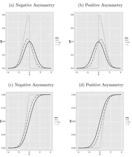
Figure 1.1 shows the behaviour ofλas a function of δ. It can be noticed thatδ approximate
−4 −2 0 2 4
−1.0 −0.5 0.0 0.5 1.0
δ
λ
Figure 1.1: λ in function of δ.
It follows straightforward from equations (1.2) and (1.3) that the mean and variance of the
standard SN distribution are, respectively,
µY =rδ, (1.6)
σY2 = 1−r2δ2 = 1−µ2Y. (1.7)
The c.d.f. of the standard skew normal is denoted by ΦSN(y;λ), and it is given by
ΦSN(y;λ) = y
Z
−∞
2φ(t)Φ(λt)dt= 2Φ2((y,0)T;0,Ω), (1.8)
where Φ2(.;0,Ω) denotes the c.d.f. of the bivariate normal distribution with mean vector 0 = (0 0)T, and covariance matrixΩ=
1 −δ
−δ 1
.
Henze (1986) proposed a standard stochastic representation of a SN variable with density
Y =d δV + (1−δ2)1/2W, (1.9) where V ∼HN(0,1) and W ∼N(0,1), forV⊥W, where HN denotes the half normal
distribu-tion. The representation in terms of convolution plays an important role in inference procedures
that involves the SN family.
Figures 1.2a and 1.2b show the p.d.f. of the standard skew normal distribution defined in
(1.5) for different values of the skewness parameter λ. The higher the value of λ, the higher
the asymmetry of the p.d.f.. Also, positive values of λ induce a positive asymmetry in the
p.d.f., and negative values of λ induce a negative asymmetry. It can be noticed that when
λ → −∞(+∞), the asymmetric distribution tends to put most of its positive mass on negative
(positive) values. In fact, the half normal distribution is a limit case of (1.5) if λ → +∞.
Figures 1.2c and 1.2d show the c.d.f. of the standard skew normal for different values of λ.
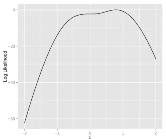
Despite its flexibility, inference for the shape parameter based on likelihood methods in the
SN family is not always possible. For instance, the likelihood can have local maximum (besides
the global maximum) and the maximum likelihood estimator can be infinity (Azzalini, 1985).
Figure 1.3 shows the log-likelihood function based on an i.i.d. sample yof size n = 1000, of Y ∼SN(0,1,1). The log-likelihood exhibits a non-quadratic shape and, as stated by
Arellano-Valle & Azzalini (2008), there is a stationary point at λ = 0. According to Azzalini (1985),
the stationary point occurs for any sample. To overcome such a problem, Azzalini (1985) also
proposed an alternative parametrization of the skew normal family distribution. Such family
is going to be briefly presented in next section.
1.2
Centered Skew Normal Distribution
In order to avoid some of the inference problems discussed in Section 1.1, such as the smooth
behaviour of the likelihood function in the neighbourhood of λ = 0, Azzalini (1985) proposed
a centered parametrization for the SN distribution, the so called Centered Skew Normal family
(a) Negative Asymmetry
0.0 0.2 0.4 0.6 0.8
−4 −2 0 2 4
y
delta
0 −0.5 −1
(b) Positive Asymmetry
0.0 0.2 0.4 0.6 0.8
−4 −2 0 2 4
y
delta
0 0.5 1
(c) Negative Asymmetry
0.00 0.25 0.50 0.75 1.00
−4 −2 0 2 4
y
cdf
delta
0 −0.5 −1
(d) Positive Asymmetry
0.00 0.25 0.50 0.75 1.00
−4 −2 0 2 4
y
cdf
delta
0 0.5 1
Figure 1.2: P.d.f. and c.d.f. of the SN(0,1,λ) for negative and positive skewness.
λ. Also, the location and scale parameters are the mean and variance of the distribution,
respectively. Azevedo et al. (2009) presented very helpful results and properties of the CSN.
To obtain the p.d.f. of a random variable Xc with distribution in the CSN family, let us
assume that X ∼SN(0,1, λ) and the following transformation
Xc =ψ
X−µX
σX
+ς, (1.10)
where ς and ψ2 are the mean and the variance of Xc, respectively, and µ
−60 −40 −20 0
−2 −1 0 1 2
λ
Log Lik
elihood
Figure 1.3: Skew Normal log Likelihood for λ.
in (1.6) and (1.7), respectively. Assuming the transformation given by (1.10) and considering
the Jacobian method, it follows from equation (1.5) that the p.d.f of Xc is given by
fCSN(xc;ς, ψ2, λ) =
2σX
ψ φ
µX +σX
xc−ς
ψ
Φ
λ
µX +σX
xc−ς
ψ
, xc ∈R. (1.11)
In order to rewrite the p.d.f of Xc as a function of the Pearson’s skewness coefficient of X,
γ, the following results are considered.
The Pearson’s skewness coefficient for a random variable X is defined by:
γ = E(X−E(X))
3
V ar(X)2/3 . (1.12)
Thus, if X ∼SN(0,1, λ),Henze (1986) proved that the Pearson’s skewness coefficient of X
is
γ =rδ3(2r2−1)(1−r2δ2)−3/2, γ ∈(−0.99527,0.99527), (1.13) where δ is defined in (1.4), r=p2/π and s=
2 4−π
1/3
After some algebraic calculations we obtain that
δ= sγ
1/3
rp1 +s2γ2/3, (1.14)
λ= sγ
1/3 p
r2+s2γ2/3(r2−1). (1.15)
Consequently, it follows that the mean and variance of X can be rewritten as functions of
γ and are given, respectively by
µX =
sγ1/3 p
1 +s2γ2/3, (1.16)
σX2 = 1
1 +s2γ2/3. (1.17)
Replacing (1.16) and (1.17) in (1.11) we obtain the p.d.f of Xc ∼CSN(ς, ψ2, γ) as
fCSN(xc;ς, ψ2, γ) =
2
p
ψ2(1 +s2γ2/3) !
φ x
c−(ς −sγ1/3) p
ψ2(1 +s2γ2/3) !
Φ g(γ) x
c−(ς −sγ1/3) p
ψ2(1 +s2γ2/3) !!
,
(1.18)
where g(γ) is given by (1.15). To simplify the presentation of the p.d.f. in (1.18), define
ς∗ = ς−sγ1/3, ψ∗ =
q
ψ2(1 +s2γ2/3).
Thus, (1.18) is rewritten as
fCSN(xc;ς∗, ψ∗2, γ) =
2 ψ∗φ
xc−ς∗
ψ∗
Φ
g(γ)
xc−ς∗
ψ∗
. (1.19)
The c.d.f. of a standard CSN variable is obtained by the integration of the density in (1.19)
ΦCSN(xc;γ) = xc
Z
−∞
2 ψ∗φ
t−sγ1/3
ψ
Φ
g(γ)
t−sγ1/3
ψ
dt. (1.20)
ΦCSN(xc;γ) = ΦSN(xσX +µX;δ),
where µX and σX are defined in expressions (1.6) and (1.7), respectively. This equivalence can
be very convenient, as there is a SN package in R (Azzalini, 2014).
From equations (1.10), (1.16), and (1.17), the stochastic representation forXc ∼CSN(ς∗, ψ2∗, γ)
becomes
Xc d= (δV + (1−δ2)1/2W)ψ∗+ς∗, (1.21)
where V and W are defined in (1.9), andδ is a function of γ as defined in (1.14).
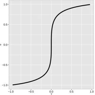
Figure 1.4 shows the relationship of delta as a function of gamma. Notice that a slight
change on γ around zero represents a strong change onδ.
−1.0 −0.5 0.0 0.5 1.0
−1.0 −0.5 0.0 0.5 1.0
γ
δ
Figure 1.4: δ as a function of γ.
As stated by Azzalini (1985), Arellano-Valle & Azzalini (2008) and Azevedo et al. (2009),
the p.d.f. defined in (1.19) is more appropriate for inference purposes if compared to the
non centered given in (1.5). According to Azzalini & Capitanio (1999), under the centered
provides better inference.
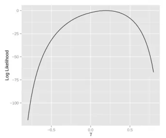
To observe this, consider a random sample x = (x1, x2, ..., xn) of Xc ∼ CSN(0,1, γ). For
such sample the log-likelihood function is
f(x|ϕ, γ) =−nln(ϕ) +
n
X
i=1
ln
φ
xc
i +sγ1/3
ϕ
+ ln
Φ
g(γ)
xc
i +sγ1/3
ϕ
. (1.22)
Figure 1.5 displays the plot based on the same sample information considered in Figure 1.3.
−100 −75 −50 −25 0
−0.5 0.0 0.5
γ
Log Lik
elihood
Figure 1.5: Centered Skew Normal Log Likelihood forγ.
Compared to the log-likelihood plot displayed in Figure 1.3, it is noticeable that the new plot
exhibits a curve with a regular behaviour, much closer to quadratic functions and without a
stationary point at γ = 0 (λ= 0).
1.3
A General Class of Multivariate skew Normal
Dis-tributions
We now define a more general distribution with Skew Normal kernel which appears in the
derivation of the conditional distributions of the MCMC algorithm proposed in Chapter 3.
This distribution was introduced, in the form presented here, by Gon¸calves & Gamerman
Arellano-Valle & Azzalini (2006). However, to adapt it to our model structure, we introduce a
new parameter to the model proposed by Gon¸calves & Gamerman (2015). As we do not use
the parametrization of Arellano-Valle & Azzalini (2006), we call this new distribution Adapted
SUN (ASUN).
Consider a d-dimensional column vectorξ, an m×d matrix W, an m-dimensional column vector η, and a d×d matrix Σ. Let us also assume column vectors U0 and U1 of dimension m and d, respectively, such that
U0
U1
∼ Nm+d(0,Σ∗), (1.23)
where Σ∗ =
Γ ∆T
∆ Σ
,Γ=Im+WΣWT,Im denotes the identity matrix of order m and ∆T =WΣ. We say that (U
1+ξ|U0+ε+η >0)∼ASU Nd,m(ξ,Σ,W,η), whereε=∆TΣ−1ξ.
Lemma 1.3.1. The density of (U1+ξ|U0+ε+η>0) is given by
f(z) = 1
Φm(ε;Γ)
φd(z−ξ;Σ)Φm(Wz−η;Im), (1.24)
where φk(.;A) and Φk(.;A) are the p.d.f. and the c.d.f., respectively, of the k-dimensional
Gaussian distribution with mean vector zero and covariance matrix A.
The proof of Lemma 1.3.1 can be found in the Appendix in Gon¸calves & Gamerman (2015).
Simulation from the density (1.24) is not straightforward. Gon¸calves & Gamerman (2015)
propose the following algorithm to efficiently sample from this distribution.
Define U∗0 = A−1U0, where A is obtained from the Cholesky decomposition of Γ, i.e,
Algorithm 1 GG Algorithm
1: Obtain u∗i from (U0∗i|U0∗ ∈B); 2: Obtain u=Au∗;
3: Obtain z∗ from (U1|U0 =u)∼N(∆Γ−1u,Σ−Γ−1∆T); 4: Obtain z =z∗+ξ;
5: return z
Step 3 in Algorithm 1 performed via MCMC, more specifically, using the Gibbs sampler,
which means that only Monte Carlo error is involved. For a detailed explanation on this
Chapter 2
Binary Item Response Models
The Item Response Theory assumes that a change in the latent variable leads to a change in
the probability of success (correct answer) in a specified item. This behaviour is described by
the Item Characteristic Curve (ICC), which specifies how the probability of an item response
changes due to changes in the ability level. The ICC is such that the probability of success will
be small for examinees with low ability, and large for examinees with high ability. It is also
important to recall that each item has its own ICC in a test.
A very important assumption on item response models (IRM) is known as Lararsfeld’s
as-sumption of local independence, which states that the examinee’s responses to different items are independent, given the latent variables. That is, the performance of an examinee in an
item cannot affect his/her performance in any other items in the test, given ability θ. This is
equivalent to say that, given ability θ, two items are uncorrelated. Also, the local independence
assures that the order of presentation of the test items must not affect the examinee’s
perfor-mance. In the case these assumptions are not held, a special model should be considered to
take testlet into account.
There are different mathematical forms of the ICC, and each of them leads to different
IRM. In this chapter some well known and employed IRM are reviewed. We focus on IRM for
binary response, and consequently models presented are meant to be applied to the analyses of
multiple choice items, corrected as right or wrong, or to the analyses of open items, when these
This chapter presents a brief review of some IRM. Section 2.1 describes the most common
IRM for binary data based on symmetric item characteristic curve. The reader more acquainted
can feel comfortable to skip this section. Section 2.2 describes some skew IRM.
2.1
Symmetric IRM
The most used models for dichotomous items are the logistic and the probit models. These
models are symmetric and they can be divided mainly into three types according to the number
of parameters that describe the item. These parameters represent features of the item such as
the discrimination power, difficulty and guessing. Another very important parameter in the
IRT, if not the most important one, is the individual’s ability (or trait), denoted by θ. We start
presenting the most simple IRM, the Rasch model.
To establish notation, through all this work,Yij is a dichotomous variable that takes 1, when
the jth examinee answers correctly to the ith item, and 0 otherwise.
2.1.1
The Rasch Model
The simplest item response model is the Rasch model (Rasch, 1960), also known as the
one-parameter logistic model (1-PL). This model involves one-parametersθj, which denotes the ability of
the jth examinee, and the item difficultyβ
i of theith item. On the Rasch model, the parameter
βi is the point on the ability scale in which the probability of a correct response is 0.5. That
is, if the ability of the examinee is higher than the item difficulty, he/she has more chance to
correctly answer the item and vice versa. This parameter can be seen as a location parameter.
An item i with βi, is said to be easier then an item k with βk, when the probability of success
at a fixed ability is higher for i in comparison to k, for βi < βk.
In the 1-PL model, the probability of a correct response in theith item by thejth examinee
is given by
P(Yij = 1|θj, βi) =
1
1 +e−(θj−βi), (2.1)
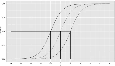
i = 1, . . . , I. In Figure 2.1, the ICCs corresponding to model in equation (2.1) are plotted for
different item difficulty levels. Notice that βi has impact only in the location, and not in the
shape of the curve. Also, notice that an examinee j with ability level 0 has P(Yij = 1|θj =
0, βi = −1) = 0.84 (solid line) and the same examinee has P(Yij = 1|θj = 0, βi = 1) = 0.16
(dashed line).
0.00 0.25 0.50 0.75 1.00
−5 −4 −3 −2 −1 0 1 2 3 4 5
θ
P(Y=1|
θ
,
β
)
Figure 2.1: ICC of the Rasch model for β = −1 (solid line), β = 0 (dotted line) and β = 1 (dashed line).
The model presented in (2.1) is not identifiable, since the same probability of success can
be obtained for two different levels of ability and item difficulty parameter. Notice that if
θ∗
j =θj + ∆ and βi∗ =βi−∆, where ∆ is a constant, we have that
P(Yij = 1|θj, βi) = [1 +e−(θj−βi)]−1
= [1 +e−(θj+∆−βi−∆)]−1
= [1 +e−(θj∗−βi∗)]−1 =P(Y
ij = 1|θ∗j, βi∗).
Therefore, for different set of parameters β and θ we can obtain the same likelihood, which
brings some inference troubles. This identification problem can be solved, for instance, by
adding a restriction on the sum of the difficulty parameters. Another way to identify the model
is by assuming a prior distribution for the abilities, which solves the identification issue by
The Rasch model is very simple, as it does not take into account more complex, but factual
scenarios. In order to turn Rasch’s model more flexible, a two-parameter model was developed
by Lord (1952), and it is presented in the next subsection.
2.1.2
Two-Parameter Models
The two-parameter models (2P) are obtained by including a discrimination parameter to the
model described in expression 2.1. The 2P model was originally developed by psychometrist
Lord (1952), who built the ICC in terms of the normal ogive curve, which is formally defined
by
P(Yij = 1|θj, ai, βi) = Φ(αi(θj−βi)), (2.2)
where Φ(·) denotes the standard normal cumulated density function (c.d.f..), and αi > 0, for
i= 1, . . . , I andj = 1, . . . , J. The constraint onαi >0 assures that an examinee with a higher
ability has higher probability of success on any item. The discrimination parameter is directly
proportional to the slope of the curve at its maximum inclination pointθ =β. Items with high
discrimination parameters are better at differentiating examinees around the location point
(difficulty), such that an small change in the latent trait lead to large changes in probability.
Figure 2.2 shows three items under the 2P model, all curves with the same difficulty
pa-rameter βi = 0, and with different discrimination values. The higher (lower) the
discrimi-nation parameter, the better (less) the item is to discriminate low and high ability around
βi. For instance, when a = 0.2 (solid line) P(Yij = 1|θj = −0.1, βi = 0, αi = 0.2) = 0.49,
and P(Yij = 1|θj = 0.1, βi = 0, αi = 0.2) = 0.51. That is, both probabilities of success
are very close. However, for a = 1 (dotted line), P(Yij = 1|θj = −0.1, βi = 0, αi = 1) = 0.46
P(Yij = 1|θj = 0.1, βi = 0, αi = 1) = 0.54. In an extreme scenario, for instancea= 100 (dashed
line), the item perfectly discriminates students in the neighborhood of β = 0. According to
Baker & Kim (2004), items whose α < 0.65 have low discrimination power; 0.65 ≤ a < 1.34
have moderate discrimination; 1.35 ≤ α < 1.69 have high discrimination, and α > 1.70 have
very high discrimination power.
0.00 0.25 0.50 0.75 1.00
−5 −4 −3 −2 −1 0 1 2 3 4 5
θ
P(Y=1|
θ
,
β
,
α
)
Figure 2.2: ICCs for the 2P IRT model for fixed difficulty parameter β = 0, α = 0.2 (solid line), α = 1 (dotted line) andα= 100 (dashed line).
two-parameter logit model (2-PL), which is formally defined by
P(Yij = 1|θj, αi, βi) =
1
1 +e−Dαi(θj−βi), (2.3)
for i= 1, . . . , I and j = 1, . . . , J, where D is a scale factor. If D = 1.7, this model provides a
reasonable approximation for the probit model defined by equation (2.2).
The quantity αi(θj −βi) is often presented as (aiθj −bi) by many authors. According to
Baker & Kim (2004) and Fox (2010), this parametrization may result in more stable
compu-tational procedures. Furthermore, under the Bayesian approach, this reparametrization leads
to conjugated full conditional distributions for (a b). This latter condition is very attractive in terms of sampling from the joint posterior distribution, and for this reason, we adopt this
parametrization all through this work.
2.1.3
Three-Parameter Models
It is noteworthy from the model defined in (2.3) and from Figure 2.2 that the probability of a
correct answer goes to zero when the ability goes to −∞. However, it is very plausible that
an examinee simply guesses an item, specially in educational tests. To take this into account,
parameter, which is a nonzero lower asymptote for the ICC. In the three-parameter model (3P)
the probability of correct response is explained by this additional factor of guessing. As in the
case of the 2P models, the 3P models are mostly defined using both the logistic (3-PL) and the
probit function (3-PP).
The three-parameter logit model (3-PL) is defined by
P(Yij = 1|θj, ai, bi, ci) = ci+
(1−ci)
1 +e−D(aiθj−bi), (2.4)
where 1< ci <0, for i= 1, . . . , I, j = 1, . . . , J, and the other quantities are defined as before.
Althoughcis commonly known as the guessing parameter, it is an item parameter’s. Therefore,
it can also be interpreted as the probability of success of examinees with extremely low ability,
being then the threshold probability of success.
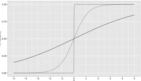
Figure 2.3 shows two ICCs varying according to parameter c, with b = 0 and a = 1 fixed.
Notice that, forc= 0.25 (dotted line), examinees with very low abilities have 0.25 of probability
of success.
0.00 0.25 0.50 0.75 1.00
−5 −4 −3 −2 −1 0 1 2 3 4 5
θ
P(Y=1|
θ
, b
, a, c)
Figure 2.3: ICCs of the 3P logistic model for b = 0, a = 1, c = 0 (solid line) and c = 0.25 (dotted line).
The three-parameter probit model (3-PP) is expressed by
where ai, bi, ci and θj are defined as in model 2.4.
A Bayesian approach for estimation and model selection for the 3PP models can be found
in Sahu (2002).
2.2
Skew IRM
All the previous models presented in Section 2.1 are based on symmetric curves. That is an
appropriated assumption whenever it is reasonable to assume that the probability of a correct
answer to an item approaches zero at the same rate as it approaches one. Under these models,
individuals with low or high abilities are discriminated in a similar way. However, it has been
emphasized by several authors that symmetric ICC’s are not always suitable to describe the
relationship between the abilities and the probability of success. To better fit ICC’s with
asymmetric behaviour, some asymmetric link functions have been proposed.
These new models take into account the skewness parameter δ, which controls the curve
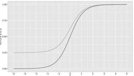
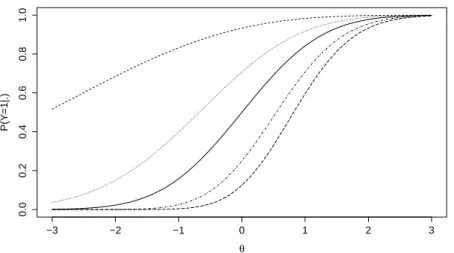
asymmetry. The parameter δ is interpreted by Baz´an et al. (2014) as apenalization parameter, since it can be seen as a penalty or as a reward on the probability of a correct answer. Figure 2.4
shows the ICC for three different values of δ. At a fixed ability level (for instance,θ = 0) when
δ = 0, the probability of a correct answer is equal to 0.5. At the same ability level, however, for
δ =−0.5, the probability of a correct answer is equal to 0.67, and forδ=−0.9, this probability
goes up to 0.86. The same happens for positive values of δ. However, in this scenario the
skewness parameter works as a “penalty”. Again, for δ = 0 and θ = 0, the probability of a
correct answer is equal to 0.5. At the same ability level however, forδ = 0.5, the probability of
a correct answer is equal to 0.33, and for δ= 0.9, this probability goes down to 0.14.
2.2.1
Skew Logit Model
We briefly describe the Logistic Positive Exponent Family proposed by Samejima (2000) and
its extension model proposed by Santos (2009).
LetYij be a Bernoulli random variable assuming 1 if the answer of the jth examinee to the
0.00 0.25 0.50 0.75 1.00
−4 −2 0 2 4
θ
cdf
0.00 0.25 0.50 0.75 1.00
−4 −2 0 2 4
θ
cdf
Figure 2.4: Cdf of standard skew normal for negative skewness (left) and positive skewness: δ =±0 (solide line), δ=±0.5 (dashed point line) and δ=±0.9 (pointed line).
follows
P(Yij = 1|θj, ai, bi, ǫi) =
1
1 +e−Dai(θj−bi)
ǫi
, (2.5)
for i= 1, ..., I and j = 1, ..., J, with ai >0,−∞< bi <∞, ǫi >0, and −∞< θj <∞. Notice
that whenǫi = 1, the symmetric link is obtained. According to Samejima (2000), the skewness
parameters ǫi represents the item complexity, which is distinct from item difficulty. This item
parameter is related to the number sequential steps to successfully solve the complete problem.
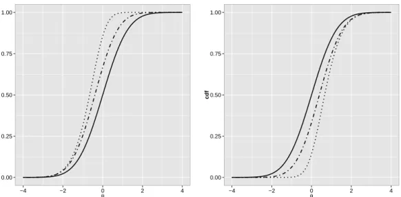
Figure (2.5) shows ICCs with parameters a = 1, b = 0 and different values for ǫ.
The proposed model by Santos (2009) extended model (2.5) by adding the pseudo-guessing
parameter c. Thus, the proposed model by Santos (2009) is given by
P(Yij = 1|θj, ai, bi, ci, ǫi) = ci+
(1−ci)
1 +e−Dai(θj−bi)
ǫi
, (2.6)
for i = 1, ..., I and j = 1, ..., J, with ai > 0,−∞ < bi < ∞,1 < ci < 0, ǫi > 0, and −∞ <
θj <∞. As in model (2.5), the symmetric three-parameter logit link is recovered when ǫi = 1.
Another contribution of Santos (2009) work is the modeling of the skewness parameters ǫi, by
−3 −2 −1 0 1 2 3
0.0
0.2
0.4
0.6
0.8
1.0
θ
P(Y=1|.)
Figure 2.5: ICCs with parameters a = 1, b = 0, c = 0, and different values for ǫ: ǫ= 0.1 (short dashed line), ǫ = 0.5 (dotted line), ǫ = 1 (solid line), ǫ = 2 (dotted-dashed line), ǫ = 3 (long dashed line).
(ǫi|πi)∼πiδ1+ (1−πi)LN(µǫi, σ
2
ǫi), (2.7)
whereδ1is a distribution degenerated in 1, andπidenotes the probability of itemibe symmetric.
Because of the complexity, the posterior distribution of all parameters are approximated via
MCMC methods, more specifically, via Metropolis-Hastings.
2.2.2
BBB Skew Probit Model
We now define the BBB Skew Probit model proposed in Baz´an et al. (2006), with some
exten-sions proposed in Baz´an et al. (2014). Let Yij be a Bernoulli random variable assuming 1 if the
answer of the jth examinee to the ith item is correct, and 0 otherwise. The BBB Skew Probit
model is defined as follows
Yij|θj, ai, bi, δi ∼ Bernoulli(pij), (2.8)
pij = ΦSN(mij;δi), (2.9)
for i = 1, ..., I and j = 1, ..., J, with ai > 0,−∞ < bi <∞,−1 < di < 1, and −∞ < θj < ∞,
and where ΦSN(mij;δi) denotes the c.d.f. of the standard SN distribution defined in 1.8. As in
the usual symmetric IRM, ai and bi denote the discrimination and difficulty item parameters,
respectively.
To avoid a Bernoulli type likelihood, the authors used the data augmentation strategy
proposed by Albert (1992), which equivalently represents the skew probit IRM defined in (2.8)
by
Yij =
1, if Xij >0,
0, if Xij,≤0,
(2.11)
where Xij =mij +eij, and eij ∼SN(0,1,−δi). For sampling purposes, the authors considered
the stochastic representation of a SN variable (Henze, 1986) assuming
eij d
=δiVij + (1−δi2)1/2Wij, (2.12)
where V ∼ HN(0,1), W ∼ N(0,1), and V⊥W. As priors specification, they elicited ai ∼
N(µa, σa2)I(ai > 0), bi ∼ N(µb, σ2b) and di ∼ U nif orm(−1,1). For θj the authors used
θj ∼ N(0,1), but also extended the SN IRM by considering asymmetrically distributed
la-tent variables, assuming, θj ∼ SN(µ, σ2, ω), where −∞ < µ < ∞, σ2 > 0, and −1 < ω < 1.
As noticed by Azevedo et al. (2011), the model considering asymmetric distribution for the
latent variable is not identifiable. To overcome this issue, Baz´an et al. (2014) assumed priors
distributions for θ hyperparameters.
2.2.3
Skew Normal model IRT under the Centered Parametrization
As mentioned in Section 1.2 of Chapter 1, because of the behaviour of the likelihood function
in the neighborhood of λ = 0 (under the original parametrization), Azzalini (1985) proposed a
centered parametrization for the SN distribution. Under this parametrization, Azevedo et al.
(2011) proposed a model based on the centered skew distribution (CSN). However, it is
impor-tant to notice that the authors did not apply the CSN to the ICC, but only to the latent trait,
literature suggest the lack of normality in the latent traits, although it is questionable if there is
a significant gain in doing so. As cited in Section 1.2, the CSN is parametrized by the Pearson’s
skewness coefficient γ, and it preserves the asymmetric behavior of the SN distribution. An
important contribution in Azevedo et al. (2011) is that the proposed model can take into
ac-count omitted responses. For estimation purpose the authors consider the Metropolis-Hasting
within Gibbs sampling algorithm.
A great advantage of the CSN if compared to the SN in item response theory is the role
of the discrimination and difficulty parameters of the item. Under the CSN distribution, the
parameters “a” and “b” play the same role in the symmetric and in the skewed models, since the
expected value and the variance of the latent distribution are invariant with respect to skewness
parameter γ. Taking into account
Xij =mij +eij, (2.13)
E[Xij] =mij and V ar[Xij] = 1, asE[eij] = 0 and V ar[eij] = 1, for both eij ∼ CSN(0,1,−γi)
and for eij ∼ N(0,1). The same does not happen when eij ∼ SN(0,1,−δi), as E[Xij] =
mij +
q 2
πδi, and V ar[Xij] = 1−
2
πδ
2
i, since E[eij] =
q 2
πδi and V ar[eij] = 1−
2
πδ
2
i.
That means that the posterior of aandbwill be very similar when considering the symmet-ric model or the skewed model under the centered parametrization, and significantly different
when considering the skewed model under the non-centered parameter. A consequence of that is
that considering the non-centered parametrization could have a negative impact on the MCMC
Chapter 3
A Flexible Class of Centered Skew
Probit IRT Model
As noticed by many authors, in many situations it is more appropriated to use an asymmetric
link for the ICC. Baz´an et al. (2014) introduced a skewness parameter associated to each item,
in order to build a more flexible model, as it allows the use of the symmetric probit as well
as the use of the asymmetric probit ICC. The authors considered a Uniform(-1,1) prior for
the skewness parameter δ. However, by eliciting this prior, the prior probability of having a
symmetric probit link, that is, δ = 0, is zero. Even more, the choice of this prior assumes
that all items are asymmetric with positive probability. It would be desirable, if not ideal, to
assume the asymmetric structure only for items that require it. Nevertheless, that information
is not available a priori and a naive model selection procedure would require 2I models to be
fitted and compared. A way to overcome this issue is to consider a mixture component for the
skewness parameter γ, so that all items may or may not be asymmetric, and in that way, the
data point out which model is more likely.
In this work, we introduce a new skew probit IRT model, in which a mixture component
on the skewness parameter is introduced, so not all items need to be assumed asymmetric
the proposed approach is that an intrinsic model selection is performed through the mixture
posterior probabilities. Our asymmetric ICC is built under the Centered Skew Normal (CSN)
distribution since centered parametrization shows some advantages over the direct
parametriza-tion (see Secparametriza-tion 1.2). Another contribuparametriza-tion of our work is that we present different algorithms
to sample from the posterior distribution (Section 3.4).
3.1
Proposed Model
Let Yij be a dichotomous variable assuming 1, if the answer of the jth, j = 1, . . . , J, examinee
to the ith, i= 1, . . . , I, item is correct and 0 otherwise. The CSN probit model is given by
Yij|pij ∼Bernoulli(pij),
pij = ΦCSN(mij;γi),
mij =aiθj −bi,
(3.1)
where ai, bi and θj are, respectively, the discriminant, difficulty and ability parameters defined
in Subsection 2.1.2,γi is the skewness parameter defined in 1.13, and ΦCSN(.) is the c.d.f of the
CSN distribution, defined in expression (1.20).
To establish notation hereafter, let θ = (θ1;. . .;θJ), a = (a1;. . .;aI)T, b = (b1;. . .;bI)T,
γ = (γ1;. . .;γI)T, and, matrix y= (yij)I×J the observed data.
The likelihood function based on an independent sample of the centered skew probit IRM
in 3.1 is given by
L(θ,a,b,γ|y) =
I
Y
i=1
J
Y
j=1
[ΦCSN(mij;γi)]yij[1−ΦCSN(mij;γi)]1−yij. (3.2)
To avoid working with a Bernoulli type likelihood, it is more convenient to work with the
stochastic representation proposed by Albert (1992), where the model presented in (3.1) can
be rewritten as
Yij =
1, if Xij >0,
0, if Xij,≤0,
where Xij =mij +eij, eij ∼ CSN(0,1,−γi) and, hence, Xij ∼ CSN(mij,1,−γ). Notice that
the skewness parameter of Xij is the opposite of the skewness parameter of the ICC as
P(Yij = 1) = P(Xij >0) = P(mij+eij >0) (3.4)
= P(eij >−mij) = 1−P(eij <−mij) (3.5)
= 1−ΦCSN(−mij;γi) (3.6)
= ΦCSN(mij;−γi), (3.7)
where the last equality is justified by the fact that ΦCSN(−x;γ) = 1− ΦCSN(x;−γ). It is
important to notice that the representation given by 3.3 preserves the probability model ofYij.
For further notation reference, let X = (Xij)I×J and x = (xij)I×J the observed realization of
X.
3.2
Prior Specifications
In order to build a more robust centered skew probit item response model (IRM) that
per-mits inference about both symmetric and asymmetric items, the following finite mixture prior
distribution for γ′
is it is assumed
γi =Zi0Wi0+Zi1Wi1+Zi2Wi2,
Zi ∼M ult(1, pi0, pi1, pi2),
Wi0 ∼δ0,
−Wi1 ∼Beta(αw, βw, ll, lu),
Wi2 ∼Beta(αw, βw, ll, lu),
pi ∼Dirichlet(α0, α1, α2),
(3.8)
where δ0 is a point-mass at zero and Beta(.) stands for the General Beta distribution defined
associated with the symmetric, negative asymmetric and positive asymmetric models,
respec-tively. The vector of probabilitypi = (pi0, pi1, pi2) is such that 2 X
k=0
pik = 1, and hyperparameters
(α0, α1, α2) are assumed to be known. For further notation reference, let Z = (Zic)I×3, where
c= 0,1 and 2.
We assume independence among the components θ, a, and b such that the joint prior
distribution is given by
π(θ,a,b) =
" I Y
i=1
π(ai)π(bi)
# " J Y
j=1
π(θj)
#
, (3.9)
where θj iid
∼ N(µ∗
θj, σ
∗2
θj),ai
iid
∼ N(µ∗
ai, σ
2∗
ai)I(ai >0), and bi
iid
∼ N(µ∗
bi, σ
∗2
bi). The hyperparameters
µ∗
ai, m
∗
bi, σ
2∗
ai and σ
2∗
bi are assumed to be known.
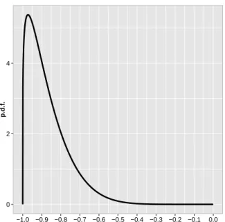
The values for αw and βw need to be carefully chosen. Firstly, the prior density cannot
concentrate too much probability mass around zero, which refers to the symmetric model and,
therefore, could lead to identifiability problems. Secondly, it cannot be strongly informative by
concentrating most of its mass in high values, which could overestimate γ. The shape of the γ
prior is shown in Figure 3.1.
0 2 4
−1.0 −0.9 −0.8 −0.7 −0.6 −0.5 −0.4 −0.3 −0.2 −0.1 0.0
γ
p.d.f
.
3.3
Posterior Distribution
The main goal of the inference process is to obtain the posterior distributions of all unknown
quantities in the model, which in our proposed model is Ψ= (X,a,b,θ,p,Z,γ). Considering the prior dependence structure given in 3.8, the joint density of (Y,Ψ) may be factorized as
π(Y,Ψ) =
I Y
i=1
J
Y
j=1
π(Yij|Xij)π(Xij|θj, ai, bi, γi)π(γi|Zi)π(Zi|pi)π(ai)π(bi)π(pi)
J Y
j=1
π(θj)
.
(3.10)
Considering the prior specifications, the joint distribution is given by
π(Y,Ψ) =
I Y
i=1
J
Y
j=1
I(Yij = 1)I(Xij >0) +I(Yij = 0)I(Xij ≤0)
fCSN(Xij;mij,1,−γi)
×
I(Zi0 = 1)I(γi = 0) +I(Zi1 = 1)fB(−γi;αw, βw, ll, lu) +I(Zi2 = 1)fB(γi;αw, βw, ll, lu)
×pZi0
i0 p
Zi1
i1 p
Zi2
i2
Γ(α0+α1+α2)
Γ(α0)Γ(α1)Γ(α2)
pα0−1
i0 p
α1−1
i1 p
α2−1
i2 fN(ai;µ∗ai, σ
∗2
ai)I(ai >0)fN(bi;µ
∗
bi, σ
∗2
bi)
×
J Y
j=1
fN(θj;µ∗θj, σ
∗2
θj)
, (3.11)
where fB(.;αw, βw, ll, lu) denotes the p.d.f. of the Beta distribution defined in Appendix 5.3,
and fN(.;µ, σ2) stands for a Normal density with mean µand variance σ2.
In the next section we introduce an MCMC algorithm to sample from the posterior (3.11).
3.4
MCMC
The model presented in (3.11) has a complex high dimensional distribution which is very hard
to be explored analytically. Despite the complexity of the proposed model, the full conditional
propose an MCMC scheme based on a Gibbs sampler with Metropolis Hastings steps.
To facilitate the MCMC construction, we reparametrize the model (3.10) taking into account
the mixture structure for γi, presented in (3.8), in the following way
γi =Zi00 +Zi1γi−+Zi2γi+, (3.12)
where γi− and γi+ denote, respectively, the negative and positive values generated for γi. By
doing this, we construct a Markov chain in γi− and γi+ instead of constructing a single chain
forγi, that is, we treat the negative and positive parts ofγi separately. Expression (3.12) shows
that, given Zi, the model is symmetric when Zi0 = 1, negative asymmetric whenZi1 = 1, and
positive asymmetric when Zi2 = 1. Therefore, model (3.10) is rewritten as
π(Y,Ψ) =
I Y
i=1
J
Y
j=1
π(Yij|Xij)π(Xij|θj, ai, bi, Zi, γi−, γi+)π(Zi|pi)π(γi−)π(γi+)π(ai)π(bi)π(pi)
J Y
j=1
π(θj)
,
=
I Y
i=1
J
Y
j=1
I(Yij = 1)I(Xij >0) +I(Yij = 0)I(Xij ≤0)
×fCSN(Xij;aiθj−bi,1,−(Zi00 +Zi1γi−+Zi2γi+))fB(−γi−;αw, βw, ll, lu)fB(γi+;αw, βw, ll, lu)
× Γ(αΓ(α0+α2+α2)
0)Γ(α1)Γ(α2)
pα0−1
i0 pα
1−1
i1 pα
2−1
i2 p
Zi0
i0 p
Zi1
i1 p
Zi2
i2 fN(ai;µ∗ai, σ
∗2
ai)I(ai >0)fN(bi;µ
∗
bi, σ
∗2
bi)
×
J Y
j=1
fN(θj;µ∗θj, σ
∗2
θj)
.
To improve the MCMC algorithm, an efficient strategy is to use a blocking scheme, where
strongly correlated parameters must be jointly sampled. For the proposed model, we consider
the following blocking scheme
(X) (θ) (a,b) (p) (Z) (γ−, γ+). (3.13)
3.4.1
Full Conditional Distribution for
X
Given parametersθ,a,bandγ, it follows from (3.13) that the components ofXare independent and such that
(Xij|θ,a,b,Z,γ,y)∼
CSN(mij,1,−γi)I(xij >0), if yij = 1,
CSN(mij,1,−γi)I(xij <0), if yij = 0.
(3.14)
That is, the full conditional distribution of Xij is a truncated CSN distribution putting
positive mass in positive values, when yij = 1, and a truncated CSN distribution putting
positive mass in negative values, when yij = 0. If γi = 0, then the full conditional distribution
of Xij is equivalent to the Truncated Normal distribution.
It is not possible to sample directly from (3.14). To do so we consider two algorithms: a
Rejection Sampling (RS) and an embedded Gibbs Sampler.
3.4.2
Full Conditional Distribution for
θ
For parameter vectorθ, the full conditional distribution can be factored for each examinee. Such
strategy does not compromise the algorithm convergence, because given the item parameters,
examinees are independent. Therefore, it is equivalent to simulate jointly all vectorθ, which has
a J-dimension distribution, or to simulate each θj separately from its marginal full conditional
distribution, which is unidimensional. The latter is more attractive because of computational
costs.
Each ability parameterθ1, . . . , θJ, given X,a,b,Z andγ, has full conditional density given
by
fN(θj;µ∗θ, σθ∗2)∝ I
Y
i=1
fCSN(xij;aiθj −bi,1,−γi)fN(θj; 0, σθ∗2), (3.15)
where µ∗
θ and σθ∗2 are the prior mean and variance of θ, respectively. After some algebraic
(3.15) for eachθj is
f(θj|X,a,b,γ)∝ I
Y
i=1
φ xij +sγ
1/3
i −(aiθj −bi)
ϕi
+ θj σ∗2
θ
!
Φ g(γi)
xij +sγi1/3 −(aiθj−bi)
ϕi
!!
,
(3.16)
where
g(γi) =
sγi1/3
q
r2+s2γ2/3
i (r2−1)
, (3.17)
and
ϕi =
q
(1 +s2γ2/3
i ). (3.18)
From expression derived in (3.16), each θj has full conditional distribution of the form
f(θj|X,a,b,Z,γ)∝φ(θj −ξθj; Σθ)ΦI(Wθj−ηj,II), (3.19)
where ΦI(.) is a normal c.d.f of dimension I, that is, given X, a, b, Z, and γ, each θj has an
ASUN distribution, defined in (1.24), denoted by
(θj|X,a,b,Z,γ)∼ASU N(ξθj,Σθ,W,ηj), (3.20)
where Σθ and ξθj are given by
Σθj =
σ2∗
θj
σ2∗
θj
PI
i=1
a2
i
ϕ2
i + 1
, (3.21a)
ξθj = Σθj
I
X
i=1
ai(xij +bi+sγi1/3)
ϕi
+ µ
∗
θj
σ∗2
θj
!
, (3.21b)
W=−a1g(γ
1)
ϕ1 −a2
g(γ2)
ϕ2 . . . −aI
g(γI)
ϕI
T
,
ηj =
g(γ1)
ϕ1 (x1j +b1+sγ
1/3 1 )
g(γ2)
ϕ2 (x2j+b2+sγ
1/3 2 )
. . . g(γI)
ϕI (xIj+bI +sγ
1/3
I )
T
,
where Σθj ∈R+, ξθj ∈R, andW and ηj column vectors of orderI.
Notice that if γi = 0 (or equivalently if Zi0 = 1), the full conditional distribution in 3.20
(θj|X,a,b,γ)∼N(ξθj,Σθj), (3.22)
where Σθ and ξθj are given, respectively, by
Σθj =
σ2∗
θj
σ2∗
θj
PI
i=1
a2
i
ϕ2
i + 1
,
ξθj = Σθj
I
X
i=1
ai(xij +bi +sγi1/3)
ϕi
+ µ
∗
θj
σ∗2
θj
!
.
Simulation from (3.20) is performed, for each fixed j, by using Algorithm 1. However, this
simulation can be computationally expensive as, at each iteration k of the MCMC, it involves
a Cholesky decomposition and the inversion of a matrix of order I ×I. Another possible way
to sample from distribution in (3.16) is to consider the Metropolis-Hastings algorithm.
The target density is given by (3.16), and as the proposal distribution we consider a random
walk given by
q(θ∗
j|θ
(k)
j ) =fN(θ∗j;θ
(k)
j , τθ2j) (3.23)
where θ∗
j is the candidate value for θj, θj(k) is the current value of the chain, and τθ2j is the
variance (tuning), which value is chosen such that the acceptance ratio is about 0.44. The
acceptance probability is given by
α(θ∗, θ(k)) = min (
1,
QI
i=1fCSN(xij;aiθj∗−bi,1,−γi)fN(θ∗j;µ∗θj, σ
∗2
θj)
QI
i=1fCSN(xij;aiθ(jk)−bi,1,−γi)fN(θj(k);µ∗θj, σ
∗2
θj)
)
. (3.24)
3.4.3
Full Conditional Distribution for (a, b)
Since parameters ai andbi are strongly correlated, a good strategy to improve the MCMC
per-formance is to generate ai and bi from the joint full conditional distribution of (a,b). However,
the full conditional distribution of (a,b) can be factored for each item, since the pairs (ai, bi)
which has a distribution of order 2×I or to simulate each pair separately from its marginal full
conditional distribution. The latter option is chosen here as it has lower computational cost.
The joint distribution for each pair (ai, bi) given X,Z, γ and θ, is given by
f(ai, bi|X,Z,θ,γ)∝ J
Y
j=1
fCSN(xij;mij,1,−γi)fN(ai;µai, σ
∗2
ai)I(ai >0)fN(bi;µbi, σ
∗2
bi) ∝
J
Y
j=1
φ xij +sγ
1/3
i −mij
ϕi
+ai−µ
∗
ai
σ∗
ai
+ bi−µ
∗
bi
σ∗
bi
!
I(ai >0)×
×Φ g(γi)
xij +sγi1/3−mij
ϕi
!!
, (3.25)
where σa∗2i and σ
∗2
bi are the prior variances of ai and bi, respectively, g(γi) and ϕi are defined in
(3.17) and in (3.18), respectively.
The joint full conditional distribution of (ai, bi|.) is the truncated ASUN distribution given
by
(ai, bi|X,Z,θ,γ)∼ASU N(ξi,Σabi,Wi,ηi)I((ai, bi)∈A), (3.26)
where A={(ai, bi)∈R:ai >0},ξi = (µai µbi)
T, Σ abi =
σ2
ai ρσaiσbi
ρσaiσbi σ
2
bi
,
ρi =
σ∗
aiσ
∗
bi
PJ
j=1θj
h
σ2∗
ai
PJ
j=1θ2j +ϕ2i
σ∗2
biJ+ϕ
2
i
i1/2
,
σb2i =
σ∗2
biϕ
2
i
σ∗2
biJ+ϕ
2
i
1 (1−ρ2
i)
,
σa2i = σ
∗2
aiϕ
2
i
σ∗2
ai
PJ
j=1θ2j +ϕ2i
!
1 (1−ρ2
i)
,
µai =σ
2
ai
PJ
j=1xijθj+sγ 1/3
i
PJ
j=1θj +ϕ2iµ∗aiσ
∗−2
ai
ϕ2
i
!
−σaiσbiρi
PJ
j=1xij+Jsγ 1/3
i −ϕ2iµ∗biσ
∗−2
bi
ϕ2
i
!
,
µbi =σaiσbiρi
PJ
j=1xijθj+sγ 1/3
i
PJ
j=1θj +ϕ2iµ∗aiσ
∗−2
ai
ϕ2
i
!
−σ2bi
PJ
j=1xij +Jsγ 1/3
i −ϕ2iµ∗biσ
∗−2
bi
ϕ2
i
!
,
Wi =
γi
ϕi
θT 1J
ηi =
γi
ϕi
xT
i +sγ 1/3
i
, (3.27)
where 1J is a column vector of ones of order J, and xi =
xi1 xi2 . . . xiJ
. The algebraic
derivation for distribution (3.26) is given in Appendix 5.2. Ifγi = 0, it implies that ϕi = 1, and
consequently distribution (3.26) becomes equivalent to a symmetric truncated bivariate normal
distribution. in this case, the full distribution of each pair (ai, bi) is given by
(ai, bi |X,Z,θ)∼N2(µabi, σ
2
bai;A), (3.28)
where A = {(ai, bi)∈R:ai >0}, and
ρi =
σ∗
aiσ
∗
bi
PJ
j=1θj
h
σ∗2
ai
PJ
j=1θ2j + 1
σ∗2
biJ+ 1
i1/2
, (3.29)
σa2i = σ
∗2
ai
σ∗2
ai
PJ
j=1θ2j + 1
!
1 (1−ρ2
i)
, (3.30)
σb2i =
σ∗2
bi
σ∗2
biJ+ 1
1 (1−ρ2
i)
, (3.31)
µai =σ
2
ai
J
X
j=1
xijθj +µ∗aiσ
∗−2
ai
!
−σaiσbiρ
J
X
j=1
xij −µ∗biσ
∗−2
bi
!
, (3.32)
µbi =σaiσbiρi
J
X
j=1
xijθj +µ∗aiσ
∗−2
ai
!
−σb2i
J
X
j=1
xij −µ∗biσ
∗−2
bi
!
, (3.33)
where σ2
ai, σ
2
bi ∈R
+, ρ
i ∈(−1,1), andµai, µbi ∈R.
Simulation from (3.26) is performed for each item i by Algorithm 1. The simulation from