Maur´ıcio Felga Gobbi
[email protected] Departamento de Engenharia Ambiental Universidade Federal do Paran´a 81531-990 Curitiba, PR, BrazilRoger Paul Dorweiler
[email protected] LACTEC, BR116 km 98 S/N Centro Polit´ecnico – UFPR Curitiba, PR, BrazilSimulation of Wind Over a Relatively
Complex Topography: Application to the
Askervein Hill
In this paper we investigate the flow of wind over a relatively complex topography at the lower portion of the atmospheric boundary-layer, by using the well known general purpose CFD package ANSYS-CFX-11. The work was motivated by the difficulty in choosing the optimal locations for turbines (micrositing) in regions of good energy potential, but with complex topography. The simulations were compared with data from landmark experiment at Askervein Hill - Scotland, in 1983. The resulting simulations also were compared favorably with the results of another package for wind simulation.
Keywords:wind turbines, atmospheric boundary-layer, Askervein, CFD
Introduction
In order to minimize the costs and maximize the efficiency of wind-generated power systems, knowledge about the spatial wind distribution is mandatory for the micrositing – that is, the identification of areas with best possible energy supply. In many developed countries, micrositing is done with the help of very dense meteorological observation networks and some standard models.
In less developed countries, meteorological data can be very scarce, and the application of those models not anchored by a robust observational base is more difficult. Besides, in many regions – for instance in Brazil – even if synoptic wind conditions are known, the overly complex geometry makes micrositing an even more difficult task (Amarante et al. , 2007).
The need to understand the topographic effects on the wind in a small scale leads to several research works, such as Jackson and Hunt (1975) development of a linear theory for the effects of the perturbation caused by mild-sloped hills in two dimensions. This theory was extended to three dimensions by Mason and Sykes (1979). Standard commercial packages for wind simulation used by the energy industry, like WAsP (Troen and Peterson, 1989) or WindMap (Brower et al. , 2002), are limited to terrains with relatively little complexity. More recently new commercial packages were developed specifically for wind-power applications, these include WindSim (Leroy, 1999) (information at http://windsim.com/) and Garrad Hassan (information at http://www.garradhassan.com/). These packages can simulate the wind over more complex terrains, including effects of boundary layer separation, and to some extent, effects of atmospheric stability.
Bowen and Mortensen (1996) introduced the Ruggedness Index (RIX), in an attempt to quantify the terrain complexity: it is the percentage of the terrain in a circular area with a 7,000 m diameter, in which the slope exceeds 18◦. If RIX exceeds 30%, the terrain is considered complex.
As a general rule, all works indicate that the wind flow over real terrains is quite variable and strongly dependent on the terrain complexity, besides the daily and seasonal variations, and stability/stratification conditions.
In this work we simulate the effects of a complex terrain on the wind flow, using a general purpose CFD package – ANSYS CFX11 (http://www.ansys.com). The simulations are done with quite high resolution to minimize grid size dependency. Several closure models for the turbulent sub-grid effects were used and compared amongst each other.
Paper received 22 March 2010. Paper accepted 31 October 2011 Technical Editor: Domingos Alves Rade
We apply the model to the Askervein Hill – Scotland, where a landmark experiment was held (Taylor and Teunissen, 1983, 1985, 1987), and compare the simulations to both measured data and WindSim model simulations found in Leroy (1999).
More recent works on wind flows over Askervein Hill using CFD include the following. Chow and Street (2009) used Askervein as a framework to show improvements over Large Eddy Simulation (LES) models by the inclusion of a mix of self-similarity and eddy-viscosity in turbulence modeling. Golaz et al. (2009) studied a one-way nested LES system applied to Askervein. Castro et al. (2003) and Stangroom (2004) used aκ-ε model to simulate flow over and around Askervein. As a follow up to Castro et al. (2003), Silva Lopes et al. (2007) modeled the flow at that same location using LES. Memon and KJondreddi (2011) tested four different turbulence closure models for the same problem.
We deliberately did not use Large Eddy Simulation (LES) modeling due to the need for higher horizontal and vertical resolution and high computational costs. For LES simulations and comparisons with other methods, see Silva Lopes et al. (2007) and Chow and Street (2009), among others.
The paper is organized as follows. In the sectionTheoretical Background and Modela short overview of the theory is shown. In The Askervein Hill Experimentwe overview the experimental data with which we shall compare the simulations. In Computational Domain and Model Setupwe discuss the domain discretization, and the model setup including boundary conditions. Then inComparisons and Resultswe show results and compare our simulations amongst themselves, with other models, and with measured data. Finally, in Conclusionswe discuss the results of the paper.
Nomenclature
∆zs = vertical grid size at the surface
EBB = squared eddy viscosity gradient g≡gi = gravitational acceleration
Lvk = Von K´arm´an length scale
k = turbulent kinetic energy P,Pi j = turbulence production
p = pressure
se = constant for turbulence closure model
S = speed-up
U = wind speed at location of interest URS = incoming wind speed at reference location
Ui = full velocity
ui = mean velocity
u′
i = velocity fluctuation
u∗ = velocity scale
uτ = sheer velocity xi = Cartesian coordinates
YR = surface roughness
z0 = roughness height
Greek Symbols
∆Y = equivalent sand grain roughness δi j = identity tensor
ε = turbulent kinetic energy dissipation rate φi j = pressure-strain correlation
κ = von K´arm´an constant µ = molecular dynamic viscosity ν = molecular kinematic viscosity νt = eddy kinematic viscosity
ω = turbulence frequency
ρ = air density
σ = constant for closure models σk = constant for closure models σε = constant for closure models σω = constant for closure models τi j = stress tensor
τw = surface sheer stress
Theoretical Background and Model
CFX is a general purpose CFD package that leans strongly towards engineering applications (especially Mechanical Engineering). Its use for geophysical applications is much less common. The package solves the three-dimensional compressible Reynolds averaged Navier-Stokes equations (RANS), plus mass conservation, energy conservation, and sub-grid equations for turbulence closure. The numerical method used by CFX solves the equations in fairly arbitrary discretized geometries using the Finite-Volume-Method.
Averaged Navier-Stokes equations
In this work we will assume that the flow is incompressible with densityρ, and the Coriolis effect is negligible. The instantaneous velocity fieldUi can be split into the average ui and a turbulent fluctuationu′
i (where Einstein’s notation is implied in a Cartesian systemxi,i=1,2,3):
Ui=ui+u′i. (1)
The same idea applies to the mean pressure field p and any instantaneous field in the problem. When substituting the above
expression into the nonlinear term of the Navier-Stokes equation a Reynolds stress symmetric tensor appears after averaging:
τi j=ρu′iu′j (2)
and needs to be modeled as it involves non-resolved scales. Reynolds stress models solve directly a partial differential equation system involving the sixτi j components. Eddy viscosity models work in a similar manner, but the sub-grid and mixing/transport effect of turbulence is accounted for in a viscous-like term.
We assume gravitational acceleration g pointing in the −x3 direction, that is: gi = (0,0,−g). Mass conservation (incompressible):
∂ui ∂xi
=0. (3)
For eddy viscosity models, the momentum reads: ∂ui
∂t +uj ∂ui ∂xj
= −ρ1∂∂
xi
p+2 3ρk
+ gi+∂∂
xj
(ν+νt)∂
ui ∂xj
, (4)
where pis the equilibrium thermodynamic pressure field, k≡u′ iu′i is the turbulent kinetic energy,νandνt are the molecular viscosity and eddy viscosity respectively,kandνt are unknowns that should contain all the effects due to the Reynolds stresses. For Reynolds stress models, the momentum equation reads:
∂ui ∂t +uj
∂ui ∂xj
=−ρ1∂∂p
xi
+gi+ ∂ ∂xj
ν∂ui
∂xj
−∂ (u′
iu′j) ∂xj
, (5)
where the last term accounts for the Reynolds stresses transport.
Turbulence closure models
To determinekandνt oru′iu′j, a closure model is needed, and in this paper we tested several options available in the CFX package, namely:
1. Zero equation model.
2. One equationk−εeddy viscosity model. 3. k−εmodel.
4. RNGk−εmodel. 5. k−ωmodel. 6. Baselinek−ωmodel.
7. SSG Reynolds stress model (Speziale et al. , 1991).
8. BaselineωReynolds stress model.
Since every closure model has some degree of arbitrariness due to the presence of constants, we have decided not to use those degrees of freedom as calibration parameters, but simply use the literature values that are recommended and set as default by the software developer (ANSYS).
Zero equation model
One equationk−εeddy viscosity model
This model is a simplified version of the traditionalk−εmodel, and was proposed by Menter (1993, 1994, 1997). The kinematic eddy viscosityνtis modeled by
∂(ρνt) ∂t +
∂(ρuiνt) ∂xi
= C1ρνt−C2ρE1e +
µ+ρνt σ
∂(νt) ∂xi
, (6)
whereµis the dynamic viscosity, and
E1e=C3EBBtanh ν
t
Lvk
2
C3EBB
, (7)
Lvkis the Von K´arm´an length scale. As in Menter (1994, 1997),C1= 0.144,C2=1.86,C3=7.0,σ=1, and
EBB=∂ (νt) ∂xi
∂(νt) ∂xi
. (8)
k−ε/ RNGk−εmodel
The equations for turbulent kinetic energykand the dissipation rateεare:
∂(ρk) ∂t +
∂(ujρk) ∂xj
= ∂
∂xj
µ+µt σk
∂
k ∂xj
+P−ρε, (9)
∂(ρε) ∂t +
∂(ujρε) ∂xj
= ∂
∂xj
µ+ µt σε
∂ε ∂xj
+ ε
k(Cε1P−Cε2ρε), (10) The turbulent kinetic energyk, the dissipation rateε, and the eddy viscosityνtare related by:
νt=Cµ
k2
ε. (11)
Pis a production term which, neglecting buoyancy and assuming incompressibility, is calculated by:
P=µt∂
ui ∂xj
∂u j ∂xi
+∂ui ∂xj
. (12)
Thek−ε(RNG-k−ε) model’s non-dimensional parameters used in this work are fixed constants in CFX and are given by:
Cµ=0.09(0.085), Cε1=1.44(1.42), Cε2=1.92(1.68),
σk=1.0, σε=1.3, (13)
while the RNG analysis suggests that the otherwise constant parameterCε1be calculated as the function:
Cε1 = 1.42−η− 1− η
4.38
1+0.012η3 ,
η =
s νt
Cµε ∂ui ∂xj
∂
ui ∂xj
+∂uj ∂xi
. (14)
k−ωmodel
The k−ω model we used was proposed by Wilcox (1986) and others. We neglected buoyancy forcing terms. The model is somewhat similar to the k−ε model but solves the turbulent frequency variableω≡ε/k. The model is suitable for lower Reynolds number computations near solid boundaries, and is very sensitive to open boundaries. We do not expect a good performance for the kind of problem we are dealing in this paper. Nevertheless, the model is included for the sake of completeness. The equations are:
∂(ρk) ∂t +
∂(ujρk) ∂xj
= ∂
∂xj
µ+µt σk
∂
k ∂xj
+P−β′ρkω, (15)
∂(ρω) ∂t +
∂(ujρω) ∂xj
= ∂
∂xj
µ+ µt σω
∂ω ∂xj
+ αω
k P−βρω
2,
(16)
wherePis calculated as in Eq. (12),β′=0.09,α=5/9,β=0.075, σk=σω=2.
Baselinek−ωmodel
The Baselinek−ω model combines thek−ω model near the surface with ak−ε(transformed tok−ω) model at the “free-stream” portion of the domain (Menter, 1993). This model fixes the open boundary problem mentioned above. The two models are blended together by a blending function. The reader is referred to Menter (1994) for details.
SSG-Reynolds stress
Reynolds stress models will predict all components of the covariances of the velocity fluctuations, the equations for the stresses transport and the dissipation rate:
∂(ρu′ iu′j)
∂t +
∂(ukρu′iu′j) ∂xk
= ∂
∂xk "
µδkl+
csρku′ku′l ε
! ∂(u′
iu′j) ∂xl
#
− 2δi jρε
3 +Pi j+φi j, (17)
∂(ρε)
∂t +
∂(ujρε) ∂xj
= ∂
∂xj
µ+µt σε
∂ε ∂xj
+ ε
k(Cε1P−Cε2ρε)
+ ∂
∂xk "
µδkl+
csρku′ku′l ε
! ∂(ε)
∂xl #
, (18)
where the production tensor
Pi j=
u′ iu′j
∂ui ∂xk
+∂uk ∂xi
The pressure-strain correlationφi jis given by:
φi j = −ρε
Cs1ai j+Cs2
aikak j−aklaklδi j 3
−Cr1Pai j+Cr2ρkSi j−Cr3ρkSi j p
aklakl
+Cr4ρk
aikSk j+Sjkaki−
2aklSklδi j 3
+Cr4ρk aikWk j+Wjkaki, (20)
where
ai j =
u′ iu′j
k −
2δi j 3 , Si j=
1 2
∂
ui ∂xj
+∂uj ∂xi
,
Wi j = 1 2
∂
ui ∂xj−
∂uj ∂xi
. (21)
The constants used in the present paper were (Speziale et al. , 1991): Cµ=0.1,se=1.36,cs=0.22,Cε1=1.45,Cε2=1.83,Cs1=1.7, Cs2=−1.05,Cr1=0.9,Cr2=0.8,Cr3=0.65,Cr4=0.625,Cr5= 0.2.
BaselineωReynolds stress model
In a similar fashion to thek−εandk−ωmodels described above, a Reynolds stress model can be derived with the turbulent frequencyω in place of an equation for the dissipationε. This model has the same advantages and limitations as thek−ωmodel, and, analogously to the previous models, a blending can be done in which, far from the solid boundaries (surface), one can use theε equation in place of theω equation, to avoid the extreme sensitivity to the unknown conditions at the domain’s open boundaries. The resulting model is what we call BaselineωReynolds stress model.
Surface layer and bottom boundary condition
The surface boundary conditions used in the present paper are based on the classic logarithmic profile (see below) of the surface layer developed by Launder and Spalding (1974). Because this application involves reasonably large scales, the grid spacing at the surface will be much larger than the viscous layer, and the no-slip condition needs to be substituted by some sort of near-wall formulation/parameterization. The average velocity at the boundary is assumed to be far enough from the viscous layer, and is linked to the sheer stress through a logarithmic function (wall-law).
The wall (surface) sheer stress is given by:
τw=ρu∗uτ, (22)
where
uτ = u
1 κln
y∗ 1+0.3YRu∗/ν
+5.2
−1
, (23)
y∗ = u∗∆Y
ν , (24)
and where κ = 0.41 is the usual von K´arm´an constant, YR is a measurement of the surface roughness,∆Y (equivalent sand grain roughness) is the vertical distance at which we have the actual modeled surface velocityu.
The Askervein Hill Experiment
The Askervein Hill project (Taylor and Teunissen, 1983, 1985, 1987) was a cooperative effort to study the flow in the low part of the
atmospheric boundary layer and how it was affected by the presence of a hill. The project was sponsored by theInternational Energy Agency ResearchandDevelopment Wind Energy Conversion Systems. This study consisted in the installation of over 50 wind measurement stations (where cup, Gill UVW, and sonic anemometers were used) which operated for two 16-day periods in September/October of 1982 and 1983. The measurements took place over and around the Askervein Hill on the west cost of the South Uist island – Outer Hebrides – Scotland (57◦11′ N, 7◦22′ W). Besides the wind measurements at the fixed stations, there were also several measurements of the weather conditions such as: TALA – Tethered Aerodynamic Lifting Anemometer – or Kite Systems, which give the wind profile up to 200 m height; and AIRsonde to give the atmospheric profile up to 2,000 m heights.
The main goal of the project was to know in great detail the wind field (mean and turbulent fluctuations) just above the ground (around 10 m) on a typical region for the installation of a wind power farm. The resulting data have become of great value for model calibration purposes. The hill has an approximately elliptic shape with axes of 2 km and 1 km, and a maximum height of 116 m above its base and 126 m above sea level. Fig. 1 shows an aerial view and the distribution of the measurement towers/posts at cross sections A-A, AA-AA, B-B. Most towers were 10 m high, but there were also towers/posts of heights 17 m, 30 m, and 50 m, and some of them measured wind at several heights. The figure also shows the locations of the stations on the top/center of the hill, HT (highest point) and CP (center point). There is also a 50 m high reference station RS (not shown in the illustration), where the reference wind is unaffected by the presence of the hill. The directions A-A and AA-AA, are aligned with the average measured wind, and also with the model’s incident wind direction.
For the sake of shortness we will not present here the resulting measurements. Some results will be presented in summarized form in a later section. For details the reader is referred to the project’s original reports.
Computational Domain and Model Setup
A computational domain was defined on the region shown in Fig. 1.
The terrain information for the present work was obtained from the Askervein Hill project as a file covering an area of 6,000 m× 6,000 m, with each point representing a projected horizontal square cell with area 23.4375 m×23.4375 m.
Modeling the terrain properly and then exporting it to match the choice of finite volumes at the bottom boundary of the domain is a quite laborious task and should not be underestimated.
Figure 1. Askervein Hill project: aerial view and measurement stations.
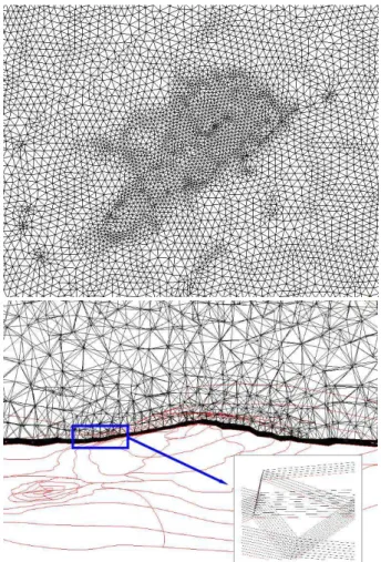
15 m above the ground, and the structured and the unstructured grids were forced to match at 15 m height. Within this 15 m region, five different structured sub-messes with grid height∆zs were used and merged with the above unstructured grid, namely: (i) 3 layers with ∆zs=5 m; (ii) 5 layers with∆zs=3 m; (iii) 10 layers with∆zs=1.5 m; (iv) 15 layers with∆zs=1 m; (v) 30 layers with∆zs=0.5 m.
Fig. 2-bottom shows a 3-D view of the bottom of the domain where the near-surface discretization can be seen.
Boundary and initial conditions
Bottom boundary
ANSYS CFX requires boundary conditions at all boundaries. We have already discussed the surface (bottom) boundary conditions used in this paper, remaining only to mention that, following the Askervein project reports, we used the surface roughness height valuez0=0.03 m. Also, the parameterYRused in this work was not the one suggested by the CFX manualYR=30z0, butYR=7.5z0, suggested by Brutsaert (1982), which is more appropriate for natural surfaces.
Figure 2. Discretized domain at the surface – horizontal view (top) and 3-D view (bottom).
Lateral and top boundaries
At the sides (lateral) and top boundaries, a zero-normal velocity condition was used (free-slip). Since these lateral boundaries are relatively far from the region of interest (center of the domain) the wall boundary condition did not seem to affect the solution. At the exit (behind the hill), a free outflow radiation condition was used. The pressure distribution used was hydrostatic, based on the local temperature and pressure conditions during the experiments.
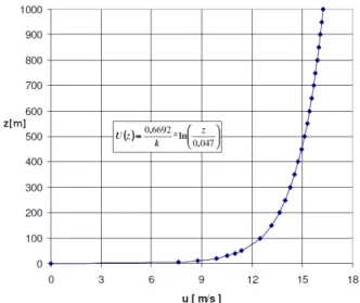
Inflow boundary
Figure 3. Profile for the inflow boundary condition.
Initial condition
In the present work only stationary results were sought and initial conditions only change the number of iterations before each run reaches the steady state. The condition used for this purpose was the inflow condition for the entire domain.
Comparisons and Results
We present the resulting simulations in terms of the speed-upS, defined as:
S=U−URS
URS
, (25)
whereU is the simulated wind speed 10 m above the surface, and URS is the wind modeled at the reference station (inlet boundary condition). All simulations are compared with the measurements (with error bar) exactly as provided by the Arkervein experiments.
Fig. 4 shows, for sections A-A, AA-AA, and B-B, comparisons between Askervein data and the zero-equation model for five different near-surface discretization, as described earlier. It can be seen that this model not only did not perform well with CFX default parameter estimation (all parameters of this model are global), but was insensitive to the grid refinement. We simply disregard this simulation for this model’s lack of physical validity.
Fig. 5 shows the results for the one-equation eddy viscosity model. Despite its relative simplicity, this model performs reasonably well over the entire range of measured points. It is a curious fact that the most all around accurate model is not necessarily the one with the most refined vertical grid size at the surface layer. We attribute this to the fact that in many cases the most refined runs showed poorer numerical convergence, probably due to the abrupt change in resolution at the structured-unstructured grid interface. Notice also that in these simulations, the sensitivity of the grid refinement varies a great deal spatially, and as a general rule, the model is less sensitive at higher locations/higher wind speeds.
Fig. 6 shows similar results but now using the two-equationk−ε model. Thek−ε is one of the most widely used closure models for turbulent flows with large Reynolds Number for its good overall results, particularly for geophysical flows. The present simulation
−1000−1 −500 0 500
−0.5 0 0.5 1
A−A distance to HT (m)
speed−up
−800 −600 −400 −200 0 200 400 600 −0.5
0 0.5 1
AA−AA distance to CP (m)
speed−up
−5000 0 500 1000 1500 2000
0.2 0.4 0.6 0.8 1
B−B distance to HT (m)
speed−up
Figure 4. Zero-equation model. Speed-up at sections A-A, AA-AA, and B-B. Near-surface∆zs: 0.5 m (thick full line), 1.0 m (thin full line), 1.5 m
(dot-dashed), 3.0 m ((dot-dashed), 5.0 m (dotted).
−1000−1 −500 0 500
−0.5 0 0.5 1
A−A distance to HT (m)
speed−up
−800−1 −600 −400 −200 0 200 400 600 −0.5
0 0.5 1
AA−AA distance to CP (m)
speed−up
−5000 0 500 1000 1500 2000
0.2 0.4 0.6 0.8 1
B−B distance to HT (m)
speed−up
Figure 5. One-equation model. Speed-up at sections A-A, AA-AA, and B-B. Near-surface∆zs: 0.5 m (thick full line), 1.0 m (thin full line), 1.5 m
−1000−1 −500 0 500 −0.5
0 0.5 1
A−A distance to HT (m)
speed−up
−800 −600 −400 −200 0 200 400 600 −0.5
0 0.5 1
AA−AA distance to CP (m)
speed−up
−5000 0 500 1000 1500 2000
0.2 0.4 0.6 0.8 1
B−B distance to HT (m)
speed−up
Figure 6. k−εmodel. Speed-up at sections A-A, AA-AA, and B-B. Near-surface∆zs: 0.5 m (thick full line), 1.0 m (thin full line), 1.5 m (dot-dashed),
3.0 m (dashed), 5.0 m (dotted).
is no exception, showing that the agreement with data is quite
satisfactory. In this case, the changes in the flow field close to
the boundary due to grid refinement were much more smooth and
uniform than for the one-equation model shown previously, which is
an indication that an extra equation for a turbulence parameter to be solved numerically and locally (rather than being set as a constant global parameter) paid off.
The flow behind the Askervein Hill (hill’s lee) can separate, and this has been reported as what happened in certain wind conditions. Although thek−εmodel performs reasonably well, we have also run the so called renormalization group analysis, or the RNGk−εmodel. This model was developed to better handle separated flows such as flows around abrupt boundary curves. The results are shown in Fig. 7. Although the model clearly shows itself as very sensitive behind the hill and able to drasticly drop in the near-ground velocity field in those separation-prone regions, the model also has poorer prediction of the velocity field elsewhere, usually under-predicting the velocity. Even at the separation region, the model showed excessive sensitivity to grid spacing, and, although no parameter sensitivity tests were performed, we conjecture that this is a difficult model to calibrate.
Fig. 8 shows the results for the k−ω model. The model performance is quite poor, and that is expected, as this model was designed for surface sub-layers with low Reynolds Number, and this type of flow regime is not resolved in the present case. Added to this, it is well known that thek−ω model is extremely sensitive to open Boundary conditions for the two turbulence parameters, and requires extremely accurate values of those at the domain entrances, something rarely known (in the present simulations we used zero gradient for all the scalar variables at the open boundaries).
−1000−1 −500 0 500
−0.5 0 0.5 1
A−A distance to HT (m)
speed−up
−800−1 −600 −400 −200 0 200 400 600 −0.5
0 0.5 1
AA−AA distance to CP (m)
speed−up
−5000 0 500 1000 1500 2000
0.2 0.4 0.6 0.8 1
B−B distance to HT (m)
speed−up
Figure 7. RNGk−εmodel. Speed-up at sections A-A, AA-AA, and B-B. Near-surface∆zs: 0.5 m (thick full line), 1.0 m (thin full line), 1.5 m (dot-dashed),
3.0 m (dashed), 5.0 m (dotted).
We also used the so calledk−ωBaseline model, which combines ak−ω model in the vicinity of solid boundaries (the surface in the present case) with ak−εmodel elsewhere. As can be seen in Fig. 9, the results were, expectedly, much better than the ones with thek−ω model alone, and the convergence rate as the grid was refined, was the most robust of all models tested here. The accuracy, compared to data, was overall worse than for thek−εmodel, and much worse at the hill’s lee. Again, even for the lower portion of the domain, the present problem has too high Reynolds Numbers to justify the use of ak−ωformulation, but we thought it would be an interesting test to see how the model would perform.
Fig. 10 shows results for what we called SSG Reynolds Stress model. This is a closure scheme that solves all six Reynolds Stress components, and the constants of the model are given by Speziale et al. (1991). The results were poorer than we expected. Similarly to what happens withk−ε models, one of the problems with the Reynolds Stress models is its poor capability of resolving near-wall (low Reynolds Number) stresses. To overcome this problem several mixed models have been proposed, amongst which the one shown here, which we call Baseline Reynolds Stress model. This model blends with ak−ωBaseline model near solid surfaces, as an attempt to overcome its weakness. The results of this model applied to our problem are shown in Fig. 11. The model performed reasonably well, except at the hill’s lee, once again.
−1000−1 −500 0 500 −0.5
0 0.5 1 1.5
A−A distance to HT (m)
speed−up
−800 −600 −400 −200 0 200 400 600 −0.5
0 0.5 1
AA−AA distance to CP (m)
speed−up
−5000 0 500 1000 1500 2000
0.5 1 1.5
B−B distance to HT (m)
speed−up
Figure 8. k−ωmodel. Speed-up at sections A-A, AA-AA, and B-B. Near-surface∆zs: 0.5 m (thick full line), 1.0 m (thin full line), 1.5 m (dot-dashed),
3.0 m (dashed), 5.0 m (dotted).
−1000−1 −500 0 500
−0.5 0 0.5 1
A−A distance to HT (m)
speed−up
−800 −600 −400 −200 0 200 400 600 −0.5
0 0.5 1
AA−AA distance to CP (m)
speed−up
−5000 0 500 1000 1500 2000
0.2 0.4 0.6 0.8 1
B−B distance to HT (m)
speed−up
Figure 9.k−ωBaseline model. Speed-up at sections A-A, AA-AA, and B-B. Near-surface∆zs: 0.5 m (thick full line), 1.0 m (thin full line), 1.5 m
(dot-dashed), 3.0 m ((dot-dashed), 5.0 m (dotted).
−1000−1 −500 0 500
−0.5 0 0.5 1
A−A distance to HT (m)
speed−up
−800−1 −600 −400 −200 0 200 400 600 −0.5
0 0.5 1
AA−AA distance to CP (m)
speed−up
−500 0 500 1000 1500 2000
−0.5 0 0.5 1
B−B distance to HT (m)
speed−up
Figure 10. SSG Reynolds stress model. Speed-up at sections A-A, AA-AA, and B-B. Near-surface∆zs: 0.5 m (thick full line), 1.0 m (thin full line), 1.5 m
(dot-dashed), 3.0 m (dashed), 5.0 m (dotted).
−1000−1 −500 0 500
−0.5 0 0.5 1
A−A distance to HT (m)
speed−up
−800 −600 −400 −200 0 200 400 600 −0.5
0 0.5 1
AA−AA distance to CP (m)
speed−up
−5000 0 500 1000 1500 2000
0.2 0.4 0.6 0.8 1
B−B distance to HT (m)
speed−up
Figure 11. Baseline Reynolds stress model. Speed-up at sections A-A, AA-AA, and B-B. Near-surface∆zs: 0.5 m (thick full line), 1.0 m (thin full line), 1.5
−1000 −500 0 500 −0.8
−0.6 −0.4 −0.2 0 0.2 0.4 0.6 0.8 1
A−A distance to HT (m)
speed−up
−800 −600 −400 −200 0 200 400 600 −0.6
−0.4 −0.2 0 0.2 0.4 0.6 0.8
AA−AA distance to CP (m)
speed−up
Figure 12. Comparison between models. Speed-up at sections A-A and AA-AA. WindSim (thick full line), CFX one equation model (thin full line), CFXk−εmodel (dot-dashed), CFXk−ωBaseline model (dashed), Baseline Reynolds stress model (dotted).
Conclusions
This paper was motivated by the need for a tool to help understanding wind over complex terrains for micrositing of wind energy plants.
Several closure methods were tested in CFX’s turbulence module when applied to the problem of wind over the Askervein Hill, for which there are extensive data available.
The authors chose not to use Large Eddy Simulations due to its computational costs.
The results showed that the k−epsilon model had the best
overall performance, with reasonably robust and smooth behavior and convergence rate as the grid size is reduced near the ground.
Finally, it is clear that the use of CFX as a tool for wind power plant micrositing is quite possible for flows over relatively complex terrain. More field experimental data sets are needed to confirm the present conclusions.
Acknowledgements
We would like to express our gratitude to LACTEC for providing support for this paper.
References
Amarante, O.A.C. do, Silva F.J.L., Parecy, E., Procopiak L.A.J., Dorweiler, R.P., Schultz, D.J., Souza, M.L. and Anunciao, S.M., 2007, “Wind Energy Resource Map of the State of Paran”, Brazil, P&D ANEEL Report – COPEL, Brazil.
Bowen, A. J., Mortensen, N.G., 1996, “Exploring the limits of WAsP the wind atlas analysis and application program”, In: Proceedings of European Union Wind Energy Conference, Goteburg, Sweden, pp. 584-587.
Brower, M., Bailey, B. and Zack, J., 2002, “Micrositing using the
MesoMap System”, Presented at Winpower 2002 Conference. Portland,
Oregon.
Brutsaert, W.H., 1982, “Evaporation into the atmosphere”, D. Reidel, Norwell, Mass.
Castro, F.A., Palma, J.M.L.M.B. and Silva Lopes, A., 2003, “Simulation of the Askervein flow. Part 1: Reynolds averaged NavierStokes equations kappaεturbulence model”,Boundary-Layer Meteorology, 107, pp. 501530.
Castro, F.A., Palma, J.M.L.M.B. and Silva Lopes, A., 2009, “Evaluation of Turbulence Closure Models for Large-Eddy Simulation over Complex
Terrain: Flow over Askervein Hill”, Journal of Applied Meteorology and
Climatology, Vol. 48, pp. 1050-1065.
Golaz, J.-C., Doyle, J.D. and Wang, S., 2009, “One-Way Nested
Large-Eddy Simulation over the Askervein Hill”,J. Adv. Model. Earth Syst., Vol. 1,
No. 6, pp. 16.
Jackson, P.S. and Hunt, J.C.R., 1975, “Turbulent Wind flow over a low
hill”,Quarterly Journal of the Royal Meteorological Society, Vol. 101, pp.
929-955.
Launder, B.E. and Spalding, D.B., 1974, “The numerical computation of
turbulent flows”,Computer Methods in Applied Mechanics and Engineering,
3(2), pp. 269-289.
Leroy, J., 1999, “Wind field simulations at Askervein hill Internal Report VECTOR AS”, Technical Report vector-9910-100, 37 p.
Mason, P.J. and Sykes, R., 1979, “Flow over an isolated hill of moderate
slope”,Quart. J. Roy. Meteorol. Soc., 105, pp. 383-395.
Menter, F.R., 1994, “Multiscale Models for Tubulent Flows.”, 24th Fluid Dynamics Conference, American Institute of Aeronautics and Astronautics.
Menter, F.R., 1994, “Eddy Viscosity Transport Equations and their Relation to the k-e Model”, NASA Technical Memorandum 108854.
Menter, F.R., 1997, “Eddy Viscosity Transport Equations and their
Relation to the k-e Model”,ASME J. Fluids Engineering, Vol. 119, pp.
876-884.
Silva Lopes, A., Castro, F.A. and Palma, J.M.L.M.B., 2007, “Simulation
of the Askervein flow. Part 2: Large eddy simulations”,Boundary-Layer
Meteorol., 125, pp. 85108.
Speziale, C.G., Sarkar, S. and Gatski, T.B., 1991, “Modelling the pressure-strain correlation of turbulence: an invariant dynamical systems
approach”,J. Fluid Mechanics, Vol. 277, pp. 245-272.
Stangroom, P., 2011, “Wind Resource Assessment in Complex Terrain Using CFD”, M.Sc. Thesis - Technical University of Denmark.
Stangroom, P., 2004, “Stangroom’,. Ph.D. Thesis - University of Nottingham.
Taylor, P.A. and Teunissen, H.W., 1983, “Askervein 82: Report on the September/October 1982 experiment to study boundary-layer flow over Askervein, South Uist”, Ontario, Canada, Meteorological Services Research Branch.
Taylor, P.A., Teunissen, H.W., 1985, “The Askervein Hill Project: Report on the September/October 1983, main field experiment”, Ontario, Canada, Meteorological Services Research Branch.
Taylor, P.A., Teunissen, H.W., 1987, “The Askervein Hill Project:
Overview and background data.”,Boundary Layer Meteorology, Vol. 39, pp.
15-39.
Troen, I., Peterson, E.L., 1989, European Wind Atlas. National Laboratory, Rskilde, Denmark, ISBN 87-550-1482-8, 656 p.