The firm size wage premium: a quantile analysis

SEMINÁRIOS DE PESQUISA ECONÔMICA DA EPGE

The firm size wage premium:

A quantile analysis

Regina Madalozzo

(lBMEC / SP)

Data: 04/04/2002 (quinta-feira)

Horário: 16h

Realização:

"

...

FUNDAÇÃO

GETULIO VARGAS

Local:

Praia de Botafogo, 190 - 11

THE FIRM SIZE W AGE PREMIUM:

A

QUANTILE ANAL YSIS

Regina Madalozzo • Ibmec - SP

March 22, 2002

Abstract

Empirical evidence shows that larger firms pay higher wages than smaller ones. This

wage premium is called the firm size wage effect. The firm size effect on wages may be attributed

to many factors, as differentials on productivity, efficiency wage, to prevent union formation, or

rent sharing. The present study uses quantile regression to investigate the finn size wage effect.

By offering insight into who benefits from the wage premi um, quantile regression helps eliminate

and refine possible explanations. Estimated results are consistent with the hypothesis that the

higher wages paid by large firms can be explained by the difference in monitoring costs that large

firms face. Results also suggest that more highly skilled workers are more often found at larger

firms .

Empirical evidence shows that larger firms pay higher wages than smaller ones.

This wage premium is called the firm size wage effect. The firm size effect on wages may

be attributed to many factors. It may be true that workers hired by large firms are more productive than those hired by small firms (Brown and Medoff, 1989; and Evans and

Leighton, 1989). It may be more difficult to monitor the labor force at large firms; this may make employers willing to pay higher wages to guarantee an efficiency wage (Oi,

1983; Akerlof, 1984; Yellen, 1984; and Kruse, 1992). Large firms may pay higher wages

than smaller ones because they want to prevent union formation (Kahn and Curme, 1987;

and Donohue and Heywood, 2000); they may even be able to share their profits with

workers (Brown and Medoff, 1989; Oi and Idson, 1999). In fact, each of these factors

could contribute partially to the differences observed between wages paid by large and

small firms. The present study uses quantile regression to investigate the firm size wage

effect. By offering insight into who benefits from the wage premium, quantile regression

helps eliminate and refine possible explanations.

A common problem that investigators face when studying wage formation is the

heteroscedastic behavior of the wage distribution (Brown and Medoff, 1989). Following

Evans and Leighton's (1989) suggestion, Oi and Idson (1999) tried to divide the sample

into different classes to lessen this effect. Quantile regression accomplishes a similar task

in a more efficient way, using alI the information available from the total sample1. All

the observations are ultimately playing a role in the maximization problem that defines

the choice of the estimated parameters at each quantile. However, the weights that these

observations have over the total function varies according the target conditional quantile.

Therefore, the outliers have smaller effects overall.

Estimated results are consistent with the hypothesis that the higher wages paid by

large firms can be explained by the difference in monitoring costs that large firms face.

1 "We have occasionally encountered the faulty notion that something like quantile regression could be

Results also suggest that more highly skilled workers are more often found at larger

firms.

In the next section, I present and examine different theories of the fmn size wage

premium. Section 2 describes the data set to be used and presents demographics for the

sample selected for use in this study. A succinct explanation of the quantile regression

method and a comparison between the results of ordinary least squares and quantile

regression are the subject of section 3. In addition, this third section analyzes the potential

reasons for the existence of the firm size wage effect and what we can conclude based on

the quantile regression approach. FinallY' in the last section, I summarize the results and

note several conclusions.

1 - Firm sue wage premium theory and applications

Using data from Italian workingwomen in textile mills, Moore (1911) related the

existence of a wage premium for those who work in larger plants. A plethora of

subsequent studies have been conducted in order to investigate the motives large firms

have for paying higher wages to their employees. From the skills differences among

workers to rent sharing and avoidance of unions' formation, different explanations have

been offered and empirically tested. Rowever, consensus has not yet been reached. In

order to understand how each explanation can be linked to the firm size wage premium,

this section examines the main models and theories used in several previuos studies.

Before entering into an explanation of the firm size wage premium, a modeling of

the firm size distribution is valuable. Lucas (1978) based his model of the firm size

distribution on the study of Kihlstrom and Laffont (1979)2. Ris model is specific to

closed economies, with a fixed amount of capital and labor, which is homogeneous with

respect to workers' productivity. The innovation ofhis study is the inclusion ofa variable

called management talent for each individual. Lucas assumes that the management talent

of an entrepreneur determines the achievable firm size.

quantiles alI the sample observations are actively in play in the process of quantile regression fitting." Koenker and HalIock (2001).

Suppose there is a closed economy with N units of labor and K units of

homogeneous capital. The combination of these factors yelds Y units of homogeneous

output. The key assumption of the Lucas' model is the existence of a continuum of

agents, with their talent following a

r

endowments for each individual x. Given their abilities, each person chooses to be an

entrepreneur or a worker. IndividuaIs who have potential profits as entrepreneurs, n, that

are higher than the competitive market wage rate, w, will comprise the management.

Those with lower ability earn more as employees than they would as managers, and

therefore they are the workers class. Consider z>O as the cutoff point, from which

individuaIs decide if they are able to be managers or workers. One key assumption of his

model is the separation between the production technology, represented by j(n,k), and the

managerial knowledge, the x g [j, k

f.

Giving a constant return technology, j(n,k)

=

n~~),

resources and labor force will maximize the output represented by

Y

N

=

z

subject to two feasibility conditions:

i) The number of workers plus the number of entrepreneurs is less than or

equal to the total population:

00

1- r(z) + fn(x)df(x) ~ 1

ii) The capital utilized is less than or equal to the total available capital:

00 K

Jk(x)df(x)

~

=

z

The solution to Equation (1) gives the multipliers w, the equilibrium wage rate,

and u, marginal return of capital. The entrepreneur income comes from the residual

between the revenue subtracted from the total wages and total capital rent,

mathematically expressed by

xg[f(n(x), k(x))] - wn(x) - uk(x) ₍₂₎

Maximization of Equation (2) permits the determination of the optimal firm size.

Using the first-order condition in relation to capital, we have

xg'(f)fk(n(x),k(x))

=

and, substituting f(n,k)

=

=

Yn,

rjJ(r)-rrjJ'(r) w

=

rjJ'(r) u (4)

Equation (4) shows that the ratio of factor prices determines the capital-labor ratio

for the firms. Substituting Equation (4) into Equation (3), we have

xg'[n(x)rjJ(r)]rjJ'(r)

=

The implicit function n(x, w, u), that is the optimal leveI of employment. Using the

cutoffvalue z and that k(z)

=

zg[n(z)rjJ(r)]

=

Equation (6) is a zero profit condition: average cosI

=

that is based on the production factors prices, managerial talent and the production

function, it is possible to determine the optimal firm size by its leveI of employment, n.

Oi (1983) extends the Lucas model to suggest that, besides the management talent

of the entrepreneur, monitoring costs influence the achievable firm size. Each manager

has to solve the following equation:

T =}J{

=

where Tis the manager production, 2 is the manager ability, and H is the result of the

fixed time endowment minus the total time required to monitor workers. Therefore, an

increase in the number of workers, N, will cause a decrease in the total manager

production, since an increase in workers means an increase in the time the manager

Equation (7) detennines the optimal finn size. This size depends both on the

entrepreneur's management talent and the time required to monitor workers. Factors À

and h, the time required to monitor each worker, establish the manager production and set

limits on finn growth. Oi explicitly derives how the substitution of labor by capital could

decrease the need for monitoring and make an increase in finn size possible.

Monitoring costs are one of the most cited reasons for the finn Slze wage

premium. Workers who have more ability would require less monitoring, and therefore

lower costs. By this reasoning, they would deserve better wages. Empirical evidence

shows that larger finns hire workers who are more able. Therefore, the difference in their

abilities, which influences monitoring costs, would result in higher remuneration of their

work compared to small finns' workers.

The efficiency wage theory can also be linked to the monitoring problem.

According to this theory, workers would receive wages higher than the optimal

competi tive leveI and can be monitored with less cost. The cost of involuntary

unemployment, raised along with wages, discourages employees shirking even without

close monitoring. Akerlof (1984) presents different paradigms that justify efficiency

wages. The most elaborate is the dual labor market hypothesis (Doeringer and Piore,

1971). Suppose the economy supports two types of jobs: the primary and the secondary

sectors. The primary sector workers are well remunerated, have stability, low quit rates, a

schedule of promotions, and investment in their human capital. The secondary sector

counterparts suffer the opposite: low wages, instability, high quit rates, little chance of

promotion, and low human capital investment. Since workers prefer the primary sector,

but its opportunity is not available to all of them, the wage paid by the primary sector is

higher than the competitive wage. However, the higher wage acts as an efficiency wage

for workers who do not want to be forced into a secondary sector job, and guarantees

worker productivity without high leveIs of monitoring.

Gibbons (1992) presents the efficiency wage hypothesis the light of game theory.

Suppose there is a repeated game in which finns have to set wages and workers decide

and the worker can accept it or remain self-employed. Given hislher acceptance, the next

step is to decide the amount of effort this worker will supply. The optimal effort is

defined by the present value ofthe worker's payoff:

(w' - e)/

Ve

=

where e is the leveI ofworker's effort, and 8 is the discount rate. Ifthe worker shirks and

is caught, then he/she willlose hislher job and receive a lower wage forever4. There is a

probability (J - p) ofbeing caught shirking. Therefore, the present value of shirking is:

V - [(1-8)w' + 8(1-p)wJ/ (9)

s - A1-~~-~

The worker's optimal behavior is to supply effort if V_e ~ _{Vs , so the present value}

of supplying effort matches or exceeds the present value of shirking. This decision

depends on the probability of being caught and the wage offered. Therefore, firms should

offer not only wages that compensate workers for hislher self-employment and disutility

of working. It should also pay a wage premium, (1-

8~(1_

more costly to workers, given the possibility of losing hislher job.

Another explanation for higher wages at larger firms is the tendency toward

avoiding workers' unionizing. There is some evidence that employers prefer to concede

more benefits to their workers to prevent the formation of unions, because unions may

lead to more difficult negotiating conditions over regular and overtime schedules of

work, increase of wages, etc. Therefore, it is believed that some part of the firm size wage

effect is related to avoiding unionization.

Brown and Medoff (1989) test this hypothesis. They believed that, if preventing

unionization was a relevant aspect of firm size wage differentials, then this effect should

be reduced for workers with a low probability of seeking unions. They verify that there is

no significant difference between these workers and those with a higher propensity to

seek unions. They conc1ude that, although efforts to avoid union formation are

Kahn and Cunne (1987) argue that lower wage workers receive more benefits

because finns fear unions. These workers have a higher propensity to join unions, since

unions increase wages and reduce wage dispersion. Using CPS data, Kahn and Cunne

find evidence that, under union threat, nonunion wage dispersion decreases, implying that

the lower end of wage distribution is the major beneficiary of this threat. Donohue and

Heywood (2000) use the same methodology as Kahn and Cunne (1987) and incorporate

the hypothesis that workers support union fonnation only if they believe their

employment conditions, i.e. to continue to be employed at the same or better leveI, will

be sustained. Donohue and Heywood question whether low-wage workers have lower

marginal productivity and, therefore, would be the first to be dismissed in the case of

union fonnation. Their empirical findings partially support the view that the finn size

wage premium derives from avoidance ofunion fonnation. For the higher and lower ends

of the wage distribution, unions are not a positive influence on wages or employment,

respectively.

Several authors5 verified that wages paid in the same establishment are positively

correlated. If in some establishment, blue-collar workers receive wages above the

average, white-collar workers will also receive higher remuneration. This positive

correlation would imply that finns with higher ability to pay prefer to share their rents.

Katz and Summers (1989) use data from 74 industries to measure the negative

correlation between wages and quit rates. They argue that the industry wage structure can

be eXplained by labor rents. In this case, the finn size wage effect is the representation of

the ability of wealthier employers to pay higher wages.

A final explanation for the finn size wage premium is the working conditions

differential between larger finns and smaller ones. Larger finns may be more likely

associated with adverse working conditions. The dissociation of the labor force from the

entire production process is considered to cause larger losses in the utility of those

4 By assumption, a worker has the possibility ofworking at this unique finn or being self-employed.

working6• Working in larger firms could make it more difficult to meet people and build

relationships with them, since larger firms can create a more impersonal work

atmosphere. A way to test this hypothesis is to include information about employees'

leveIs of pleasure in working7 or including very detailed occupational variables. Brown

and Medoff (1989) do not find evidence to support the working conditions hypothesis.

In the next sections, I will present the Ordinary Least Squares (OLS) and Quantile

Regression estimates of the firm size wage premium. Using the 1999 CPS and the 1998

NLSY, I will test and analyze the hypotheses presented in this section. The hypothesis of

paying a wage premium to avoid unionization will be tested by the inclusion of a union

indicator. If this inclusion modifies significantly the firm size or/and plant size variables,

a share of the explanation may be attributed to this cause. The rent sharing, the working

conditions and the workers ability differential theories will be tested by the inclusion of

industries and occupations indicators. Better the specification ofthe wage equation, lower

is expected to be the firm size wage effect. Using the NLSY98 data, the ability

differential among workers will be tested using the variable ASV AB, which represents

the respondents results to the Armed Services Vocational Aptitude Battery. Finally, the

monitoring cost idea will be analyzed in the light of the descriptive characteristics of the

quantile regression method. Having different magnitudes and significance leveIs for the

different quantiles may indicate returns specifically for the workers who deserve higher

or lower degree of monitoring on their work. For instance, it will be seen on the next

sections, when analyzing the CPS99 results, that the lower conditional quantiles receive

higher returns for firm size than the upper quantiles. This result may be indicating that the

workers who deserve more monitoring, the ones located at the lower quantile, receive an

efficiency wages.

6 Usually, microeconomics considers leisure as a good and work as the opposite. However, in practice,

workers can increase their leveI of utility by doing something they Iike. Inability to control the whole process of production is generally considered to decrease the utility of work. An alternative way to understand this effect is by considering that work always causes disutility. Still, the dissociation ofthe entire process causes a larger disutility to the worker.

2 -Data and Demographics

Two datasets are used in the present study: the Current Population Survey (CPS)

and the National Longitudinal Survey of Youth (NLSY). The latter database has fewer

observations and a more restricted sample than the former, since it includes only persons

that were between 14 and 21 years old in 1979, however some of its features are relevant

to this investigation, such as its panel structure and more specific questions.

The U.S. Census Bureau conducts the Current Population Survey (CPS) monthly.

It interviews over 50,000 households and gathers information on various areas of interest

such as: education, labor force status and participation, demographics, and others. The

sample used in the present study is the March 1999 Survey. Although this study uses only

the March 1999 Survey, the March files have existed since 1962 and they contain the

Annual Demographic File and the Income Supplement. While the March file has changed

some of its questions over the years, different years of the March file are recommended

for wage analysis because this series combines demographic information8 and details

about labor force participation9. The March 1999 CPS file is especially interesting for the

present study since it contains a specific firm size variable, divided in six categories:

fewer than 10 employees, between 10 and 24 employees, between 25 and 99 employees,

between 100 and 499 employees, between 500 and 999 employees, and 1,000 or more

employees.

Table 1 presents some demographic information for the sample. The first colurnn

describes the most general sample. It contains 29,513 observations for men, between ages

20 and 60, inclusive. The average individual is 39 years old, with an annual income of

39,067 dollars. He is white, completed high school, and is married. A large portion ofthe

sample, 39.5%, works in a firm with 1,000 or more employees. The second colurnn

restricts the sample to full-time workers10 and those who were engaged in the labor force

for at least 48 weeks per year. In this second sample, 24,233 men are included. Age, race,

8 For instance: age, race, education, marital status, residence area, etc. 9 Such as: wages, industry, occupation, firm size, etc.

educational pro file, and finn size participation remain similar to those in the first sample.

The average annual income, increased as expected, to 43,614 dolIars per year.

FinalIy, the sample that will be used in this investigation restricts the individuaIs

to those who eam at least 4 dolIars per hour and are not top coded by their incomell• The

variable hourly wage is constructed by dividing annual wage and salary income by the

number of hours usually worked per week multiplied by the number of weeks worked last

year12. This sample is based on 23,292 observations ofmen between 20 and 60 years old,

inclusive, full-time workers, and who worked during at least 48 weeks in the year before

the interview. The average individual in this sample is 39 years old, white, married, and

did not complete a college degree. The mean hourly wage in the sample is $18.75.

Finn size is a variable is divided into six categories, according to the total number

of employees in alI organization plants13. As cited before, the categories are: fewer than

10 workers, 10 - 24 workers, 25 - 99 workers, 100 - 499 workers, 500 - 999 workers and

1,000 or more workersl4. In the final sample, roughly 37% of the respondents work for

finns with fewer than 100 employees. The majority of the other 63% of the sample work

for f1ID1s with 1,000 or more employees (41%).

The National Longitudinal Survey (NLS) is a study sponsored by the Bureau of

Labor Statistics. It is composed by a set of surveys designed to gather infonnation at several points in time on the labor market experiences of diverse groups of men and

women. From the six NLS samples, the one used in this study is the National

Longitudinal Survey of Y outh (NLSY), with a sample of boys and girls that were

11 The importance of restricting the wages to those equal or higher to some mini mal amount, in this case,

four dollars, is to avoid errors in the answers. The majority of observations that were dropped had declared thernselves to earn less than 7,000 dollars per year from wages and salaries and to work more than 35 hours per week, 48 weeks per year. I. e., to be full time workers who receive much less than the minimal wage. 684 observations were dropped because they had computed wages that were abnormally low. Concerning top coded observations, only 257 individuais declared receiving wages and salaries above the maximum wage dec1arable by CPS. Regressions were made including them and results are similar to the ones presented here at ali.

12 This ca1culation results in the houriy wage. The same method is used in other studies, for example Evans

and Leighton (1989).

13 Evans and Leighton (1989), and Oi and Idson (1999) report results with the inclusion of a plant size

variable. This variable does not exist for the March files.

14 These categories are valid after 1992. From 1962 to 1991, there were only 5 categories. The first one was

between 14 and 21 years old on the last day of 1978. The investigation of the

respondent' s labor force performance and attachrnent, and education and training

investment are the main purposes of the NLSY. However, its actual content is much

broader than that, inc1uding questions about military participation, vocational aptitude,

school performance, alcohol and substance use, fertility, and child care.

For the present paper, three points about the NLSY must be highlighted. First, the

NLSY contains variables that measure the implicit ability of each person in its sample.

The NLSY respondents were tested following the Armed Services Vocational Aptitude

Battery (ASVAB) criterial5. Either the results of these tests can be used to capture the

ability of the respondent on specific subjects, or the raw and percentual scores may be

used to obtain a measure of the respondent's "abilities" on general matters. This feature

of NLSY is important to this study, since it constitutes the only variable that actually

captures differences in workers implicit abilities. The inc1usion of the ASV AB variable in

the last specification of the wage equation indicates if the usual measures of skills make

some difference on the wage differentials between firms of dissimilar sizes. Second, the

panel structure of the NLSY may help to seize another kinds of influences that may lead

to the firm size wage differences. Using panel data, a specific variable relative to each of

the respondents is inc1uded in the regression and eliminates doubts about unobserved

personnel differences influencing wage's formation. The panel structure of the NLSY

helps the understanding of the same factor as the ASV AB variables. However, results

differ since the use of a specific variable is different from the analysis made by the use of

each individual response over time. The panel structure captures a lot more than the

ability differences between each individual. It also computes personnel differences that

cannot be sized by a particular variable. Finally, the NLSY contains two variables on the

size of firms. One is the number of employees at the plant where the respondent works. In

contrast to the CPS, the NLSY reports the actual number of employees, instead of an

indicator variable. The other variable is an indicator for the size of the firm, which is also

15 The ASV AB consists of a battery of tests that measure knowledge and skill in the areas of general

informative. This variable assumes a value of 1 if the whole firm has more than 1,000

employees and zero otherwise. Therefore, using the NLSY data it is possible to infer both

the plant size and the firm size effect over wages, which cannot be made using the

CPS99, which does not contain a plant variable.

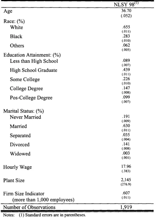
Table 2 reports the demographics for the NLSY98. Once more, the sample is

restricted to men, however restrictions about income and hours of work are not made,

since the number of observations is much lower than in the CPS sample. This youth

sample is based on 1,919 observations of men between 34 and 41 years old, inclusive.

The average individual in this sample is 36.7 years old, white, married, and did not

complete a college degree. The mean hourly wagel6 in the sample is $17.96. The average

number of workers at each plant is more than 2,000, and the majority of the sample works

for firms with 1,000 or more employees (60.7%).

3 - Ordinary least squares and quantile regression: the empirical evidence

Much attention has been devoted to the firm size wage effect. Different methods

and various datasets can be used with the same objective. While some authors use data

from individuaIs or from firms to investigate the firm size wage effect, there is a more

recent trend ofusing employer-employee matched data to do the same thingl7. Although

this is a valuable approach, the present paper will rely entirely on employee answers to

investigate firm size, and it will be comparable with Brown and Medoff (1989), Evans

and Leighton (1989) and Oi and Idsen (1999).

Using data from individualsl8 and establishmentsl9 separately, Brown and Medoff

(1989) test the main hypothesis about the firm size wage effect. Using ordinary least

squares estimation and appropriate corrections for unspecified heteroskedasticity, they

conclude that the firm size wage effect exists even when grouping individuaIs by specific

speed; auto and shop infonnation; mathematics knowledge; mechanical comprehension; and electronics infonnation. See NLSY79 User's Guide for more detail.

16 NLSY reports the hourly wage.

17 Haltiwanger, Lane, Spletzer, Theeuwes and Troske (1999) present a compilation ofpapers with

estimatives conceming the finn size wage effect from matched data.

18 As the Current Population Survey (CPS) and Quality of Employment Survey (QES).

19 Namely: the Survey of Employer Expenditures for Employee Compensation (EEEC), the Wage

characteristics (e.g., union status, industry), and that the effect comes both from the plant

and from the firm size. They conclude further that the effect derives mainly from the

higher quality of the workers, because they are not able to confirm the effects of

unionization, better working conditions, higher ability to pay, smaller supply of labor or

elevated monitoring costs that might have motivated the higher wages in larger firms.

Evans and Leighton (1989) use both the May 1983 CPS and the 1981 data from

the National Longitudinal Survey (NLS) of Young Men to investigate the same effect.

Their conclusions, based on ordinary least squares regressions and first differences

estimators, are that the firm size wage effect exists and that the plant effect can be

neutralized by properly controlling for the total number of employees at all sites. They

also suppose that the reason larger firms pay higher wages is a matter of how they

evaluate workers' characteristics; i.e., larger firms recruit workers with higher degrees of

education and training, and the firm size wage effect is derived from this se/ectíon of

workers.

Based on 1993 CPS data, Oi and Idson (1999) use a different approach to

investigate the effect of firm size on wages: the bivariate association between firm size

and selected variables. They estimate that a man with selected characteristics could earn

an additional 45.2% working in a firm with 1,000 or more employees as he would have

earned if he worked in a firm with fewer than 25 employees. U sing the May 1983 CPS, in

order to control for small and large establishrnent size, they conclude that the wage

difference between larger and smaller firms could decrease to 27.8% if adequate controls

are added.

These three studies conclude that the firm size wage effect exists and, for lack of

stronger evidence toward another factor, that this difference between wages is generated

by the higher skills of larger firms' workers. My paper will develop the idea of wage

formation along the lines of these three previous studies.

The main innovation of this study is the use of quantile regression. By using this

method, it will be possible to investigate the firm size wage effect along the conditional

results and compares them with the findings from previous studies. After that, the second

sub-section describes the quantile regression method and results.

3.1 - Ordinary least squares results

The objective of this paper is to better understand the effect of firm size on wages.

The sample is restricted to men; between 20 and 60 years old, inclusive; full-time

workers, i.e. working at least 35 hours per week; and those who were engaged in the

labor force for at least 48 weeks during the year that precedes the CPS interview.

Restrictions were also made by dropping individuaIs who eam less than four dollars per

hour or are top coded by their wage and salaries' income20. The estimation of a wage

equation based on two different methods, namely ordinary least squares and quantile

regression21, follows Equation 10:

13 6 11 7 6

ln(wage)

=

"IJJ;X;

r;

;=1 ;=1 ;=1 ;=1 ;=2

where:

Xi represents age, age squared, indicator variables for race (Categories: white,

black, and others. The excluded category is "white".), education (Categories: less than

high school, high school degree, college dropouts, vocational degree, college degree,

graduate degree, with the excluded category "less than high school".), and marital status

(Categories: never married, married, separated, divorced, widowed. The excluded

category is "married".);

Zi represents indicator variables for central city status (indicator variable that

equals 1 if the person resides in a central city (SMSA) and zero otherwise), region of

residence (Categories are: northeast, north central, south and west. The excluded category

is "south".), and union membership (indicator variable that equals 1 if the person is

member of a union and zero otherwise);

/nd represents two-digit industry;

Occ represents one digit occupation;

FirmSize represents finn size indicators with 6 categories22, with the exc1uded

category "fewer than 10 employees".

F olIowing the suggestions of Brown and Medoff (1989), the indicator for union

membership, and the industry and occupation indicators were inc1uded one at a time,

each inc1usion representing a new specification. Results from a basic regression

compared with the estimations that inc1ude the union indicator may shed light on the

suspicion that large finns pay larger wages to prevent unionization of their workers. The

additions of industry and occupation indicators imply a more direct control for labor

quality, i.e. workers' unrneasured ability, and particular trends of specific industries and

occupations. Table 3 presents the results for these three specifications.

Not much difference can be seen between the estimated coefficients from the

alternative specifications. The return to the variable age, of approximately 5%, is positive

and significant for alI regressions. The concave behavior of the wage profile, is

confinned by the coefficient of age squared, which is negative and significant in alI

specifications. Expected results are reached for the race and education indicators. White

males earn from 8 to 20% more than non-white males, while education has a positive and

increasing returno Indicators for marital status show that married men, the exc1uded

category, are better remunerated than non-married men23.

The inc1usion of the union membership indicator does not change the finn size

indicators' estimated coefficients. Being a union member, as suggested by previous

papers, has a positive effect on wages.

The final estimation in Table 3 is the most complete mean wage equation.

Inc1usion of industry and occupation categories does not alter the magnitude of the

21 Quantile regression coefficients and confidence intervals were estimated using S-Plus Package. The OLS

results were estimated in Stata.

22 The categories are: 1 =fewer than 10 employees,

2=\0-24 employees, 3=25-99 employees, 4= 1 00-499 employees, 5=500-999 employees and

coefficients on the demographic, residential, and union indicator very much.

Nevertheless, there are some differences concerning the firm size wage premium. In

colurnns 1 and 2, the firm size indicator for firms with 10 to 24 employees revealed a

wage effect of 9%24 in relation to those working in firms with fewer than 10 employees,

the exc1uded category. The larger firm size indicator, i.e. for firms with more than a

thousand employees, had an effect of 22%. Colurnn 3 shows a stable estimated

coefficient in the firm size wage effect for the category of firms with lOto 24 workers of

9%, however, there is a decrease in the effect for larger firms employees, from 22 to

20%.

The NLSY98 was used to estimate the model specified in Equation (10). Given

particular characteristics of these data, four specifications were tested. The first one

inc1udes age, age squared, indicator variables for race (Categories: white, black, and

others. The exc1uded category is "white".), education (Categories: less than high school,

high school degree, college dropouts, college degree, graduate degree, with the exc1uded

category "less than high school".), and marital status (Categories: never married, married,

separated, divorced, widowed. The exc1uded category is "married".); and indicator

variables for central city status (indicator variable that equals 1 if the person lives in a

central city (SMSA) and zero otherwise), region of residence (Categories are: northeast,

north central, south and west. The exc1uded category is "south".). To deal with the plant

and firm size wage effects, two variables were inc1uded. The first one is the logarithmic

value of the actual number of employees at the plant where the respondent works25. To

deal with the firm size, an indicator for firms that have more then 1,000 employees was

inc1uded.

23 Several papers direct attention to the subject of wage difTerences between married and non-married men in the U.S. For example, see: Korenman and Neumark (1992), and Waite (1995).

24 Firm size wage efTect = ePi -1, where

/li

25 Alternative regressions using the actual number of employees as the plant size, instead of the logarithmic

Following the same pattern revealed by the CPS99 results, not much difference

can be seen between the estimated coefficients of the alterna tive specifications presented

in Table 4. However, the significance of some variables varies widely between

regressions. For instance, the variables age and age squared follow the expected behavior

only in the first specification, the baseline regression. In the more complete version, the

one that includes an ability measure, neither of these variables is significant. Concerning

race, education and marital status, NLSY regressions reinforce the CPS results, where

white males earn more than non-white males, education has a positive increasing return,

and married men receive higher wages than non-married men.

The inclusion of the union membership indicator does not significantly change

either the plant size variable or the firm size indicator' estimated coefficients. Being a

union member, as suggested by previous papers, has a positive effect on wages.

The third estimation in Table 4 is the one that includes occupation and industry

indicators in the wage equation. Inclusion of industry and occupation categories changes

the magnitude of the coefficients of the education, union indicator (lower), and plant size

variables. The plant size wage effect that was more than 2% decreases to 1.5% after this

latter inclusion of variables. The effect on the firm size indicator does not change

significantly.

The last column of Table 4 presents the results for the most complete estimation

of the wage equation. The fourth specification includes a variable that measures the

percent scores on the ASV AB test, described in the previous section. This variable was

included with the intention of measuring part of the ability differential among

respondents, and, with this, to separate this effect from the plant and firm size wage

effects. Besides the unexpected results on the age and age-squared variables, the

estimated coefficients for the other variables remain similar. Results for the plant size and

firm size variables do not change much either in magnitude or significance. The plant

size wage return is 1.4% and, the firm size, is roughly 5%.

Overall, ordinary least squares results confirm the previous fmdings of the

clarify reasons for the firm size wage premi um. Linear regression cannot support or

disprove some explanations that focus on preventing union formation, efficiency wage

premiums, or employee monitoring, given the available variables from the data set.

Differences in workers' abilities are the only explanations that can be currently assessed

using the ordinary least squares regressions, particularly by the inclusion of occupation

and industry indicators, and the ASV AB results, in the NLSY sample. A brief description

of the quantile regression approach and its advantages compared to the linear regression

follows, along with the description of results.

3.2 -Quantile regression approach and results

One of the challenging points of this study is the econometric tool used to analyze

the firm size wage effect: quantile regression. Using the same principIes that make the

ordinary least squares result in the conditional mean estimation, Koenker and Bassett

(1978)26 introduced quantile regression as the estimator of the conditional quantile

function. This innovative approach brings not only more explanatory power to the results

when compared to the details captured by the least squares approach, but also decreases

the influence of outliers in the estimations.

The least squares approach solves the minimization problem:

(11 )

Equation (11) results in the conditional mean function E(y\x). Quantile regression

proceeds in the same way, directing its attention to the p-dimensional optimization

problem:

(12)

26 See also Koenker and D'Orey (1987), Koenker and Portnoy (1996), Buchinsky (1999), and Koenker and

Using linear programmmg methods, Equation (12) results in the conditional

quantile functions. The p represents a loss function that can be calculated conditioned to

each selected quantile r, where r E

(0,1}27.

Some benefits of quantile regression are especially interesting in the present

study. Its low sensitivity to outliers is one. In the linear squares regression, the failure of

the normality assumption, especially with outliers that result in a long-tail distribution,

results in a poor estimation of parameters. Quantile regression estimations, imposing

different weights on observations according to the quantile to be estimated, are robust

even for cases with a distribution far from Gaussian. A second plus of quantile regression

is its descriptiveness. OLS regression estimators, as a conditional mean estimation,

present a result for the average point. Quantile regression opens the possibility of

multiple estimators for the same variable depending on the targeted quantile.

These two advantages of quantile regression over OLS estimation have been

highlighted for their importance in the present study. Even with the increased number of

observations in the sample to be investigated, the income distribution does not follow a

normal distribution. The presence of outliers and their influence on the estimations can be

seen in the next section. The leveI of descriptiveness achieved by quantile regression

helps us answer fundamental questions. For instance, quantile estimations are very good

at answering the question of which workers benefit most from large firms' employment.

A final note about how to interpret the estimated coefficients: as in the OLS

regression the interpretation of the coefficients is made by evaluating the partial

derivative of the dependent variable, Y, with respect to one of the regressors, X;. In

quantile regression, the procedure is the same; only now, the partial derivative is of the

conditional quantile of the dependent variable in relation to one of the independent

variables, X;. I.e., the interpretation comes from : ;

=

Pi

targeted quantile. However, the reader should keep in mind that the observation

27 Robust standard errors are available to each quantile using the modified Barrodale and Roberts (1974)

method, as described in Koenker and D'Orey (1987).

belonging to the r - quantile in one conditional distribution may not belong to the same quantile with changes in its covariates (Buchinsky, 1998).

The wage equation, Equation (10), was estimated using the procedures explained

in the previous section. Table 5 and Figures 1 - 3 present the results for the firm size

indicators of the CPS99 sample. Table 6 and Figures 4 to 7 present the results for the

NLSY98 sample28, with regressions that include both the plant and firm size wage

effects, and separated specifications for the inclusion of these variables separately. For

the both samples, the observable trend of decreasing retum of plant andlor firm size, as

the quantiles get higher, is the same for all sets of estimations; the variability is related to

the confidence intervals in each specification.

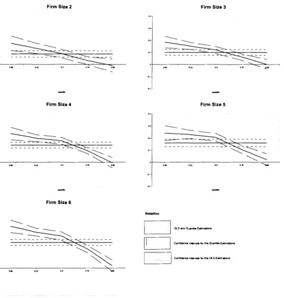
Conceming the CPS99 sample, the trend for all regressions is a higher wage

retum in relation to the firm size variable for the lower quantiles and a lower retum, even

zero return, for the higher ones. The lower quantile, the 5%, has a retum of 19% for the

second fmn size category and more than 30% for the sixth firm size category. The 95%

quantile, the highest one estimated, has no significant returns, positive or negative, for

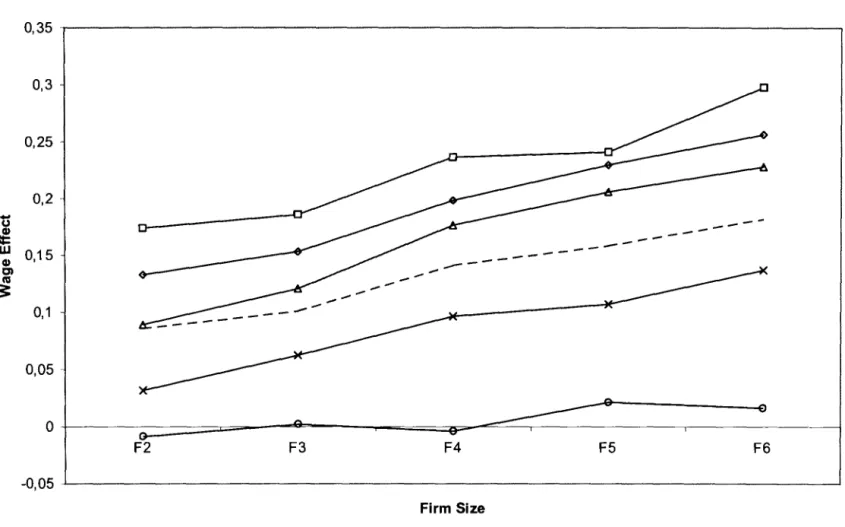
any of the firm size categories. Figure 8 tries to show in a more intuitive way the CPS99

quantile regression results compared to the OLS estimations. Recall that the firm size

variable is not continuous for the CPS, therefore we have one indicator variable for each

different firm size category. On the vertical axes, we measure the firm size effect on

wages. The upper line represents the retum achieved by the workers that belong to firms

that have between 10 and 24 employees, so called "firm size 2". The lower line

represents the firm size wage retum for the workers of the larger firms, the ones with

more than 1,000 employees. This graph does not affirm that workers in larger firms

receive lower wages than the ones at smaller fmns. It is showing that the retum to the firm size is larger for the small firm' s workers than for the larger firm' s workers.

For the regressions that do not include occupation and industry indicators,

specifications 1 and 2, the quantile regression results are significant1y different from the

finn size increases along with the number of employees that each category represents.

For the category 2, finns with lOto 24 employees, individuaIs belonging to the 5%

quantile have wages 19% higher than the individuaIs in the same quantile that work for

finns with fewer than 10 employees. For the 5% quantile, retums vary between 21 %, for

the category 329, to 37%, for the category 6, which includes finns with 1,000 or more

workers.

The closer the estimations get to the 75% quantile, the more the results from the

quantile regression approach the ordinary least squares estimates. Retums vary between 4

and 16% for this quantile, given each finn category in relation to the excluded one. At the

95% quantile, neither one ofthe categories present positive or negative retums to the finn

size indicators.

The regression that includes occupation and industry indicators, specification 3, is

different from the ordinary least squares estimation for the lowest and highest quantiles;

however, for the middle quantiles, i.e., 50%, and 75%, results are not significantly

different. Only for the finn size categories 4 and 630 are retums to finn size significantly

different from linear regression results for the majority of the quantiles. For the latter

category, workers in the lower quantile, 5%, have retums to finn size 34% higher than

the individuaIs from the excluded category do. This retum decreases as the quantiles get

higher: for the 25% quantile, retum is 29%; for the 50%, retum is 26%; for the 75%

quantile, retum is 15%; and, for the higher quantile, 95%, the retum is not significantly

different from zero.

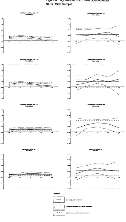
The NLSY98 sample maintains the results reached by the previous related

regressions on the CPS99 sample. Figures 4 and 5 present the results. The difference

between them is that Figure 4 preserves the same scale for both the plant size and the

finn size variables, while Figure 5 puts the plant size on a different scale. In these figures,

one can notice that the plant size effect follows a pattem similar to the one presented by

28 Estimated coefficients for the other variables, for the samples of CPS99 and NLSY98, are presented in

the Appendix A.

29 I.e., firms with 25 to 99 employees.

the finn size indicators on the CPS99 sample31. There is a positive and significant plant

size effect on the lower quantiles for the specifications 1 and 2 that is reduced to zero on

the 95% quantile. An interesting result is that, on the latter specifications, the plant size

effect is significant only for the middle and upper quantiles, not being significant for

lower end of the conditional distribution. The finn size wage effect, presented at the right

side of Figures 4 and 5, only is significant and positive for the middle quantiles in all

specifications.

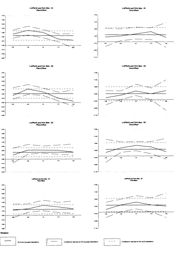
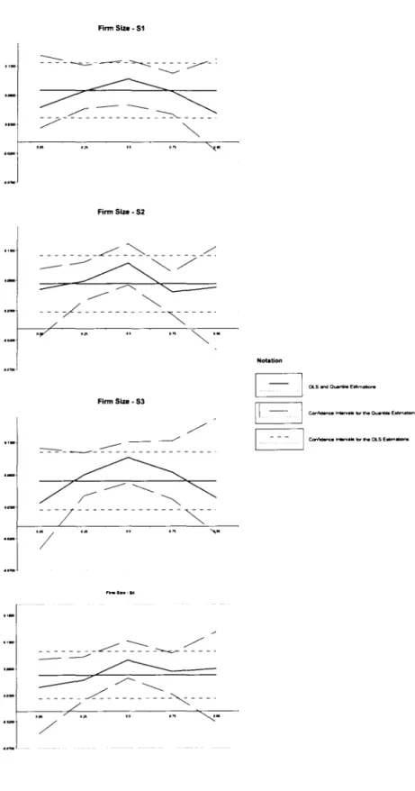
Figures 6 and 7 present the results for all four specifications, however now

including only the plant size or the finn size variables. The same pattem revealed on the

previous figures is clear here. The plant size wage effect appears to be significant only for

the middle quantiles and upper quantiles, especially for the regressions that include better

measures of specific workers' ability32. The finn size wage effect also is maintained as

significant for only the middle quantiles for all specifications. Both ends of the quantile

regression present no significant effect for these variable.

Quantile regression estimations, by disaggregating the mean effect, make the

analysis of the estimated results to be much deeper than when using OLS. A different

retum for each quantile in the same finn size category is inconsistent with the hypotheses

of rent sharing and bad working conditions as possible explanations for the fmn size

wage premium. If this wage premium carne from finns able and willing to pay more for

their labor force, as the rent-sharing hypothesis predicts, we would expect a surplus to be

paid to the higher quantile in each category and we cannot verify that this happens.

According to the results presented before, the higher conditional quantile receives no

significant retum to the finn size variable, using the CPS results, or receives a smaller

retum than the lower quantiles, using the NLSY data. Without that surplus, this

explanation can be dropped.

31 lt was suggested that the CPS finn size variable may be actually capturing the plant size instead ofthe

number of employees at all1ocations. This cannot be tested here, however the NLSY98 results are consistent with this.

32 Specifications 3 and 4, those inc1ude the occupations and industries indicators, and the ASV AB

The suggestion that the finn size wage premmm originates In bad working

conditions is also not consistent with the findings. If worse labor conditions existed at

large finns, alI quantiles should receive a premium with an increase in finn size.

However, the highest quantile, as described before, does not receive wage premiums at

alI.

The explanation that larger finns pay higher wages to prevent union fonnation is

also not sustained by presented estimations, neither by ordinary least squares, as in

Brown and Medoff (1989), nor by the quantile regression approach. The inclusion of a

variable related to union membership does not significant1y alter results to the finn size

indicators. Therefore, the present study is also inconsistent with this hypothesis.

Many authors have cited differences in workers' abilities as the cause for the finn

size wage effect if no other explanation can be found in the estimated models. However,

the true skill of a worker is an implicit measure. It is not adequate to measure skilI by education achieved, because persons with the same degree of education may have very

distinct skilIs. The effort that workers take to complete their tasks, which could also

imply a difference in skilIs, is also not easily measured.

Brown and Medoff (1989) use infonnation about leveIs of responsibility as a

measure of ski11. They conclude that the finn size wage effect declines with an increase in

skilI leveI (for example, among white colIar occupations such as managers and

professionals). They also assume that any finn size wage effect stems from differences

between large and smalI finns' abilities to measure workers' skilIs. This set of

conclusions implies that blue-colIar workers receive the premiums available at larger

finns because their skills are more easily measured. In the present study, Figures 1-3

show those workers in the lower conditional quantile of the wage distribution can achieve

a large impact on their own wages by working at a large finn. Thus, results presented

here are in accord with the previous literature.

Although not the best way to measure skills or abilities, the differences between

educational degrees in the finn labor supply is also used to this end. Evans and Leighton

characterize ability by leveI of education and stability in a job. Table 7 presents the

proportion and the frequency of workers at each degree of education classified by firm

size based on the CPS sample33. Results are similar to those from previous studies: the

larger the firm, the larger the proportion of workers with college degrees or more. For

firms with fewer than 10 employees, 29.7% ofworkers have college or graduate degrees.

Firms with 1,000 or more employees have this estimative increased to 40%. The same

rationale works for lower degrees of education as well. Only 6.2% of the workers who

belong to a firm with 1,000 or more employees have less than a high school degree, in

comparison to 17% for firms with fewer then 25 employees. Even if one chooses to

measure ability by the imperfect variable of educational degree, there is some indication

that more highly skilled workers are allocated preferentially to larger firms.

In the effort to better control for workers ability, the NLSY98 was used. Although

it contains fewer observations than the CPS, this sample helps to explore whether better

measures of workers ability change the conclusions, but can partially explain the

difference on the wages among firms of different size34. The introduction ofthe plant size

variable showed that the upper conditional quantile has positive retums to it, even if the

retum to the firm size variable is not significant.

As a final point, estimates shown in this paper suggest that the firm size wage

premium can be partially explained as an efficiency wage to compensate for monitoring

costs. Small firms can monitor their workers at lower costs than larger companies.

Knowing this difference in the cost of monitoring, larger firms would pay larger wages to

their employees in order to guarantee that they work efficiently with low supervisiono As

described in the first section, this efficiency wage both compensates workers for their

lower supervision and imposes a larger penalty for those caught shirking. In addition,

efficiency wage payment is an altemative for those firms whose monitoring costs are toa

33 Appendix C presents two figures about the workers' education distribution among firms of different size.

34 Appendix B shows the results for 6 different specifications of a wage equation estimation based on a

high. The efficiency wage theory points out that workers who deserve more monitoring

may receive higher wages as a way to incentive them to do their work better.

The employees who typically have their work monitored are at the lower

quantiles. These workers have a direct superior who controls their production. The

workers at the upper quantiles have more independence in the way they can act;

monitoring their work does not necessarily mean watching the way the person is working.

Instead, results signal the quality of their work.

The importance of quantile regression can be seen here. Using OLS, it is more

difficult, if even possible, to conclude that low ability workers receive larger premiums

for working in larger firms than workers at the opposite end of the distribution. The idea

of dividing the sample between blue-collar and white-collar workers and estimating their

wage effects35 was intended to check for the same aspects that quantile regression

presents. However, with quantile regression, a more efficient way to consider the total

information from the sample is achieved, since it uses the information from the entire

distribution to estimate the coefficients for every quantile.

The results derived in this paper are consistent with at least two of the theoretical

reasons discussed. The larger effects of the firm size wage difference apparently comes

both from differences in workers' skills and from higher monitoring costs at larger firms.

Both of these factors are accepted by other authors and verified with the quantile

regression approach.

4 - Conclusion

The previous literature has not been entirely successful at analyzing the possible

reasons for the firm size wage effect. Empirical applications to deal with the subject were

restricted to ordinary least squares regressions and the analysis of the partitioned sample

by characteristics. Brown and Medoff (1989) investigate different databases in a careful

way with the objective of discovering the most influential causes of the firm size wage

premium. They conclude that differentials between workers' abilities are responsible for

the greatest part of this wage premium. Oi and Idson (1999) gather conclusions from

several authors, at different periods, and also conclude in favor of the higher abilities

presented by large firms' workers to justify the wage differential of these workers relative

to those who are employed at small firms. Meanwhile, several authors argue in favor of

avoidance of unions by large firms (Kahn and Curme, 1987), rent sharing (Katz and

Summers, 1989), or efficiency wages (Akerlof, 1984; Yellen, 1984; and Kruse, 1992).

The present study uses the Current Population Survey from March 1999 to investigate

these hypotheses and employs an innovative technique for the analysis: the quantile

regression approach.

The use of quantile regression improves the previous analyses by allowing more

of the sample information in the estimation of each coefficient and at the same time

estimates coefficients for different points of the conditional distribution. One of the

advantages of quantile regression is its low sensitivity to outliers. Even when the sample

fails to fulfill the normality assumption, quantile regression, imposing different weights

to observations according to the quantile to be estimated, has robust estimators. A second

benefit of quantile regression is its descriptiveness. Quantile regression, opens the

possibility of multiple estimators for the same variable depending on the targeted

quantile, and portrays the behavior of the estimation for different points of the variable

distribution. In contrast with linear regression estimators, quantile estimations permit a

profound knowledge of the sample characteristics, by supplying conditional estimated

coefficients at selected quantiles.

Skills or abilities are not easily measured, but with the available evidence, there is

evidence consistent with the hypothesis that workers at large firms are better prepared to

do their jobs. Monitoring costs are not explicit either. The conjunction of the results that

better skilled workers are allocated to larger firms and that these workers receive

supervision36 receive higher firrn size wage premiums than the workers who do not need

h " 37

as muc momtonng .

Examination of the data and regression results, especially the results pointed out

by the panel data regressions, shows that it is possible to support the ideas that the

differentials in workers' abilities and in the costs of monitoring play a relatively large

role in the firrn size wage effect. While the firrn size wage premium varies from between

19 and 37% for the 5% conditional quantile, depending on the firrn size indicator

analyzed, returns are not significantly different from zero for the 95% conditional

quantile for any of the firrn size indicators. Results from quantile regression and its

conditional quantile analysis reinforce the arguments in favor of monitoring costs and

efficiency wages being paid by larger firrns, and is not consistent with the hypotheses of

rent sharing and poorer working conditions at those firrns.

36 UsuaJ1y the ones at the lower conditional quantiles.

References

Akerlof, G.A. (1984) "Gift Exchange and Efficiency-Wage Theory: four views

American Economic Review (Papers and Proceedings), Vol. 74, pp. 79-83.

Barrodale, I. and Roberts, F. (1974) "Solution of an overdetermined system of

equations in the LI Norm" Communications ofthe ACM, VoI. 17, pp. 319-320.

Brown, C. and Medoff, J. (1989) "The Employer Size-Wage Effect" The Joumal of

Polítical Economy, Vol. 97, Issue 5, pp. 1027-1059.

Buchinsky, M. (1998) "Recent Advances in Quantile Regression Models: a Practical

Guideline for Empirical Reseach" Joumal of Human Resources, Vol. 3, Issue 1,

pp.88-126.

Calvo, G. and Wellise, S. (1980) "Technology, Entrepreneurs, and Firm Size" Qurterly

Joumal ofEconomics, VoI. 95, pp. 663-78.

Doeringer, P. and Piore, M. (1971) " Internai Labor Markets and Manpower Analysis "

Health Lexington Books. (book)

Donohue, S. and Heywood, J. (2000) "Unionization and Nonunion Wage Patterns: Do

Low-Wage Workers Gain the Most?" Joumal ofLabor Research, VoI. 21, Issue 3,

pp. 489-502.

Evans, D. and Leighton, L. (1989) "Why Do Smaller Firms Pay Less?" The Joumal of

Human Resources, VoI. 24, Issue 2, pp. 299-318.

Gibbons, R. (1992) "Game Theory for Applied Economists" Princeton University Press.

(book)

Haltiwanger, J.; Lane, J.; Spletzer, J.; Theeuwes, J. and Troske, K. (1999) "The

Creation and Analysis of Employer-Employee Matched Data" EIsevier Science

B.V.

Kahn, L. and Curme, M. (1987) "Unions and Nonunion Wage Dispersion" Review of

Economics and Statistics, VoI. 69, pp. 600-07.

Katz, L. and Summers, L. (1989) "Industry Rents: evidence and implications"

Kiblstrom, R. and Laffont, J. (1979) "A General Equilibrium Entrepreneurial Theory

of Firm Formation Based on Risk Aversion" Journal of Political Economy, VoI.

87, Issue 4, pp. 719-48.

Koenker, R. and Bassett, G. (1978) "Regression Quantiles" Econometrica, VoI. 46,

Issue 1, pp. 33-50.

Koenker, R. and D'Orey, V. (1987) "Computing Regression Quantiles" Applied

Statistics, VoI. 36, Issue 3, pp. 383-93.

Koenker, R. and Hallock, K. (2000) "Quantile Regression: an Introduction"

Department of Economics, University of Illinois at Urbana-Champaign.

(forthcoming in the Joumal of Economic Perspectives "Symposium on

Econometric Tools ").

Koenker, R. and Pornoy, S. (1996) "Quantile Regression" Working paper, University

ofIllinios at Urbana-Champaign, ORWP number 97-0100.

Kruse, D. (1992) "Supervision, Working Conditions, and the Employer Size-Wage

Ef!ect" Joumal ofIndustrial Relations, V. 31, Issue 2, pp. 229-49.

Korenman, S. and Neumark, D. (1991) "Does Marriage Real/y Make Men More

Productive?" The Joumal ofHuman Resources, v. 24, n. 2, pp. 282-307.

Lucas, R. (1978) On the Size Distribution of Business Firms" The Bell Joumal of

Economics, VoI. 9, Issue 2, pp. 508-23.

Moore, H. (1911) "Laws ofWages" Mackmillan. (book)

Novo, A. A. (2000) "Openness and Money Growth: Dynamic Consistent Monetary

Policy? And an Empirical Assessment with Quantile Regression" Mimeog.

Oi, W. (1988) "Heterogeneous Firms and the Organization of Production" Economic

Inquiry, VoI. 21, pp. 147-71.

Oi, W. and Idson, T. (1999) "Firm Size and Wages" in: Handbook ofLabor Economics,

VoI. 3, edited by O. Ashenfelder and D. Card, pp. 2165-2214.

Slicbter, S. (1950) "Notes on the Structure of Wages." Review of Economics and

Statistics, VoI. 32, pp. 80-91.

Weiss, L. (1966) "Concentration and Labor Earnings" American Economic Review,

VoI. 56, pp. 96-117.

Yellen, J. (1984) "Efficiency Wage Models of Unemployement" American Economic