Liao’s method for a few space and time fractional reaction-diffusion equations arising in Engineering

(1)

Liao’s method for a few space and time

fractional reaction-diffusion equations

arising in Engineering

R.Rajaraman1 and G.Hariharan2

Department of mathematics, School of Humanities & Sciences SASTRA University, Thanjavur-613 401, Tamilnadu, India

1

rraja@maths.sastra.edu

2

hariharan@maths.sastra.edu

Abstract_{— In this paper, we have applied an accurate and efficient homotopy analysis method (HAM) to} find the approximate/analytical solutions for space and time fractional reaction- diffusion equations arising in mathematical chemistry. The method provides solutions in rapid convergence series with computable terms. To the best of our knowledge, until now there is no rigorous HAM solutions have been reported for the space and time fractional reaction-diffusion equations (FRDEs). Some numerical examples are presented to demonstrate the validity and applicability of the method. The power of the manageable method is confirmed. Moreover, the use of HAM is found to be accurate, efficient, simple, flexible and less computation cost.

Keyword- Homotopy analysis method, fractional derivatives, space and time fractional reaction diffusion equations

I. INTRODUCTION

In recent years, notable contributions have been made to the applications of fractional differential equations (FDEs). These equations are increasingly applied to efficient model problems in research areas as diverse as machanical systems, dynamical systems, control, chaos,continuous time random walks, anomalous diffusive and subdiffusive systems, wave propagation and so on. The fractional calculus and its applications (that is, the theory of integrals and derivatives of any arbitrary real or complex order) has gained considerable popularity and importance during the past three decades or so, mainly due to its applications in diverse fields of science and engineering [1,5,6]. Mathematical modelling of complex processes is a major challenge for contemporary scientist. In contrast to simple classical systems, where the theory of integer order differential equations is sufficient to describe their dynamics, fractional derivatives provide an excellent and an efficient instrument for the description of memory and hereditary properties of various complex materials and systems.

The diffusion of two or more chemicals at unequal rates over a surface react with one another in order to form stable patterns is represented by reaction diffusion equation. The nature of the diffusion is characterized by temporal scaling of the mean square displacement

r t

2

( )



t

α.For standard diffusion α=1, whereas in anomalous sub diffusion α<1 and in anomalous super diffusion α>1. Standard diffusion is represented by classical diffusion equations and sub diffusion and super diffusion are represented by fractional diffusion equations. In last few decades fractional differential equations are increasingly using in the modelling of various physical and dynamical systems. The most important advantage of using fractional differential equations is their non-local property. It is well known that integer- order fractional operator but the fractional order differential operator is a nonlocal operator. This indicates that the next state of a system depends not only upon its current state but also upon all of its previous states. Recently, Das [2] had applied the variational iteration method for fractional order diffusion equations. Hariharan et al. [14,15] introduced the Haar wavelet method for some nonlinear parabolic equations.

Recently, various iterative methods are applied for getting numerical and analytical solutions of linear and nonlinear fractional reaction-diffusion equations [3,4,7,8,9,10-13]. The homotopy analysis method (HAM) was introduced by Liao [16,18-20]. The proposed method has been used by many mathematicians and engineers to solve various equations based on homotopy, which is a basic concept in topology. In recent years, HAM has been successfully employed to solve many types of nonlinear homogeneous or nonhomogeneous equations and systems of equation as well as problems in science and engineering [4,7,8,9,10,17,21]. More recently, Hariharan [17] applied the HAM for Kolmogorov-Petrovskii-Piskunov (KPP) and fractional KPP equations. The validity of the HAM is independent of whether or not there exist small parameters in the considered equation. HAM provides us with a simple way to adjust and control the convergence of solution series.

(2)

,

0

2 U

U

c

t

x

α

∂

=

<

≤

∂

(1) Here the diffusion is Markovian.

The second type is the time fractional diffusion equation

2

U

c

t

x

β β

∂

=

∂

(2) Here the diffusion is non-Markovian and can be further be divided into

0 <

β

<

1

which has sub diffusive behaviour and

1 <

β

<

2

which has a super diffusive behaviour.

The third type is mixed case with both space and time fractional derivatives

U

c

t

x

β α

∂

=

∂

(3) The outline of this paper is as follows. In section 2, we review the basic idea of Liao’s method. In section 3, we present the application of the HAM to space and time fractional reaction-diffusion equations (FRDEs) and also some numerical examples are provided for demonstrating the applicability and validity of the method. Also a conclusion given in section 4.

Definitions of fractional derivatives and integrals

In this section, we have given some notations, definitions and preliminary facts that will be used further in this work. The Caputo fractional derivative allows the utilization of initial and boundary conditions involving integer order derivatives, which have clear physically interpretations. Therefore, in this paper we shall use the Caputo derivative

D

α proposed by Caputo in his work on the theory of viscoelasticity. In the development of theories of fractional derivatives and integrals, it appears many definitions such as Riemann-Liouville and Caputo fractional differential-integral definition as follows.

(1) Riemann-Liouville definition:

( )

(

)

( )

(

)

1

,

;

1 , 0

1 .

m m R

t

a t m

m m

a

d f t

m

N

dt

D f t

f T

d

dT

m

dt

m

t T

α

− +



=

∈



=





_≤

_{− <}

_<



Γ

−

₋





Fractional integral of order

α

is as follows:

( )

(

)

(

)

( )

1

0

1 ,

0.

t R

a

I

t

f t

t T

f T dT

α

_α

α

− −

=

−

>

Γ −



(2) Caputo definition:

( )

(

)

( )

_{( )}

(

)

1

,

;

1 , 0

1 .

m m c

m

a t t

m a

d f t

m

N

dt

D f t

f

T

dT

m

_{t T}

α

− +



=

∈



=





_≤

_{− <}

_<



_Γ

₋





II. BASIC IDEA OF HAM

In this section the basic ideas of the homotopy analysis method are introduced. Here a description of the method is given to handle the general nonlinear problem.

=0, t>0, (4)

(3)

Let denote the initial guess of the exact solution of Eq. (4), h an auxiliary parameter, an auxiliary function and L an auxiliary linear operator with the property.

, when . (5)

The auxiliary parameter h, the auxiliary function , and the auxiliary linear operator play important roles within the HAM to adjust and control the convergence region of solution series. Liao [16,18] constructs, using

,

as an embedding parameter, the so-called zero-order deformation equation.

;

,

(6)

Where

;

is the solution which depends on h,

,

, and q. when q=0,the zero-order deformation Eq.(4) becomes

;

, (7)

and when q=1, since h and , the zero-order deformation Eq.(6) reduces to,

;

,

(8)

So,

;

is exactly the solution of the nonlinear Eq.(6). Define the so-called

m

th order deformation derivatives.

_! ;

(9) If the power series Eq.(6) of

;

converges at q=1, then we gets the following series solution:

∑

.

(10) Where the terms can be determined by the so-called high order deformation described below.

B. High- order deformation equation Define the vector,

u

_n

{

u t u t u t

₀

( ) ( )

,

₁

,

₂

( )

,...,

u t

_n

( )

}

→

=

(11)

Differentiating Eq.(6) m times with respect to embedding parameter q, the setting q=0 and dividing them by ! , we have the so-called

m

th order deformation equation.

, , (12) With initial condition

u

m

(

0 )

=

0

Where = ,

, (13) and

,

_! ; (14)

For any given nonlinear operator , the term

,

can be easily expressed by Eq.(14). Now the solution of the

m

th order deformation Eq.(12) for

m

≥

1

becomes

(

)

[

R

u

t

]

c

J

t

r

hH

t

u

t

u

_m

(

)

=

_m

(

)

_m−1

(

)

+

(

,

)

_t _m _m−1

,

+

α

χ

(15)

where c is the integration constant determined by the given initial condition and

{

}

ξ

α

d

f

t

f

J

n

t

(

)

(

)

(

1 )

(

1

0

−



−

Γ

(4)

Thus, we can gain , … …. by means of solving the linear high-order deformation Equation one after the other order in order. The

m

th order approximation of u(t) is given by

∑ .

(17) III.APPLICATIONS OF LIAO’S METHOD

Example: 1 We consider the time fractional Gas dynamic equation

2

1 (

)

(1

)

0, 0

1,

0

2 u

u

t

x

α

∂

+

−

=

≤

≥

∂

(18) With initial condition u(x,0)=a (a constant) (19)

We will apply the Liao’s method to solve Eq.(18) subject to the initial condition Eq.(19) We define the nonlinear operator as

[

]

(

,

;

)

(

,

;

)

(

1 (

,

;

)

2

1 )

;

,

(

)

;

,

(

2

q

t

x

q

t

x

q

t

x

t

q

t

x

q

t

x

N

φ

_α

φ

α

−

∂

+

∂

=

(20) and linear operator

[

]

α

_φ

φ

t

q

t

x

q

t

x

L

∂

=

(

,

;

)

;

,

(

(21) With the property

L(c1(x))=0 (22)

Where c1 (x) is the integration constant. Now by using Eq.(12) we have

[

_m₋₁

]

=

m

U

R

(

,

;

)

(

,

;

)

(

1 (

,

;

)

2

1 )

;

,

(

2

q

t

x

q

t

x

q

t

x

t

q

t

x

φ

α α

−

∂

+

∂

(23) and the solution of the mth order deformation Eq. (12) for m≥1 becomes

[

(

,

)

(

)

]

)

,

(

)

,

(

₁ 1 ₁

1 −

− −

−

=

m m

+

m m

m

x

t

U

x

t

L

hH

r

t

R

U

u

χ

(24)

Since m≥1, χm=1 and under the rule of solution expression suggested by Liao [16] we set the auxiliary function

H(r,t)=1 and also this equation has sub diffusive behavior we obtain the following successive approximations as

u

₀

(

x

,

t

)

=

a

( )

(

)

(

1 )

1 ,

1

+

Γ

−

=

α

t

a

t

x

u

(

)

( )

(

)

(

)

( )

(

3

1 )

1

2

2 )

2

1 (

1 )

,

(

3 2 2

2

+

Γ

+

−

+

Γ

−

=

α

α α

t

a

t

a

t

x

u

The final solution in a closed form is

(

)

( )

(

)

( )

(

)

( )

(

)

2 3

( )

2

4 2

( , )

(1

)

(1

)(1 2 )

(1

)(1 6

6 )

1

2

1

3

1 (1

)(1 2 )(1 12

12 )

...

4

1 t

t

u x t

a

t

a

α α

α

= +

−

+

−

+

−

+

Γ

+

Γ

+

Γ

+

−

+

Γ

+

(5)

( )

,

1

t t

ae

u x t

a

ae

=

− +

(26)

Example: 2 We consider another nonlinear homogeneous gas dynamic equation

0 ,

1

0 ,

0 )

1 (

)

(

2

1

2

≥

≤

=

−

∂

+

∂

t

x

u

x

u

t

u

(27)

With initial condition

u

(

x

,

0 )

=

e

−x

t

(28) We will apply the Homotopy analysis to solve Eq.(27) subject to the initial condition

Eq.(28)

We define the nonlinear operator as

[

]

(

,

;

)

(

,

;

)

(

1 (

,

;

)

2

1 )

;

,

(

)

;

,

(

2

q

t

x

q

t

x

q

t

x

t

q

t

x

q

t

x

N

φ

_α

φ

α

−

∂

+

∂

=

[

φ

]

α

φ

_α

t

q

t

x

q

t

x

L

∂

=

(

,

;

)

;

,

(

L(c1(x))=0 (31)

[

m−1

]

=

m

U

R

(

,

;

)

(

,

;

)

(

1 (

,

;

)

2

1 )

;

,

(

2

q

t

x

q

t

x

q

t

x

t

q

t

x

φ

α α

−

∂

+

∂

(32) and the solution of the mth order deformation Eq.(12) for m≥1 becomes

[

(

,

)

(

)

]

)

,

(

)

,

(

₁ 1 ₁

1 −

− −

−

=

m m

+

m m

m

x

t

U

x

t

L

hH

r

t

R

U

u

χ

(33)

H(r,t)=1 and also this equation has sub diffusive behavior we obtain the solution as follows



=

+ −

+

Γ

−

=

n k

k k x

k

t

e

t

x

u

0

) 1 (

)

2 (

)

1 (

)

,

(

α

(34)

When α=1 we get the solution in closed forms

u

(

x

,

t

)

=

e

−x

(

1 −

e

−t

)

(35)

Fig,1 Comparison of solutions of Eq.(27) for some values of t and x=0.5 using 4th_{term HAM approximation}

with α=0.25(blue curve),α=0.5(green curve),α=0.75(red curve)

0 0.1 0.2 0.3 0.4 0.5 0.6 0.7 0.8 0.9 1

(6)

Fig.2 The surface area shows u(x,t) for the Eq.(27) using fourth term approximation of HAM with α=0.5 for some values of x and t (x=t)

Example 3: Consider the biological population equation as follows:

(

,

)

(

,

))

(

₂

,

))

(

,

),

0 ,

0

1

2 2

2 2 2

≤

<

>

+

∂

+

∂

=

∂

α

α α

t

x

u

y

t

x

u

x

t

x

u

t

x

u

(36) with initial condition

u(x,y,0)=

x

+

y

(37)

0

0.1 0.2 0.3 0.4

0.5 0.6 0.7

0.8 0.9 1

0 0.1 0.2 0.3 0.4 0.5 0.6 0.7 0.8 0.9 1 0 0.002 0.004 0.006 0.008 0.01 0.012

0

0. 2

0. 4

0. 6

0. 8

1

0 0.

5 1

(7)

We will apply the HAM to solve Eq.(36) subject to the initial condition Eq.(37) We define the nonlinear operator as

[

(

,

;

)

]

(

,

;

)

(

,

;

))

(

,

;

))

2 (

,

;

)

2 2 2 2 2

q

t

y

x

y

q

t

y

x

q

t

y

x

t

q

t

y

x

q

t

x

N

φ

_α

φ

α

−

∂

−

∂

−

∂

=

[

]

α

φ

t

q

t

y

x

q

t

x

L

∂

=

(

,

;

)

;

,

(

L(c1(x))=0 (40)

[

_m₋₁

]

=

m

U

R

(

,

;

)

(

,

;

))

(

,

;

))

(

,

;

)

2 2 2 2 2 2

q

t

y

x

y

q

t

y

x

q

t

y

x

t

q

t

y

x

φ

α α

−

∂

−

∂

−

∂

(41) and the solution of the mth order deformation equation Eq.(12) for m≥1 becomes

[

(

,

)

(

)

]

)

,

(

)

,

(

1 ₁

1

1 −

− −

−

=

m m

+

m m

m

x

t

U

x

t

L

hH

r

t

R

U

u

χ

(42) Since m≥1, χm=1,we set h= -1, H(r,t)=1and also the equation has sub diffusive behavior we obtain the final

solution as

(

)



∝

=

Γ

+

=

0

1 )

,

(

k

t

y

x

t

x

u

α

α (43)

Example:4 Consider the time fractional advection dispersion equation

1

0 ,

0 ),

,

(

)

,

(

)

,

(

)

,

(

2 2

≤

<

>

+

∂

−

∂

=

∂

α

λ

α α

t

x

u

x

t

x

u

b

x

t

x

u

D

t

x

u

(44)

Where D=2, b=2 and λ=1

u(x,0)=ex (45) Now we will apply the Liao’s method to solve Eq.(43) subject to the initial condition Eq. (45).

[

(

,

;

)

]

(

,

;

)

2 (

,

₂

;

)

(

,

;

)

(

,

;

)

2

q

t

x

y

q

t

x

q

t

x

t

q

t

x

q

t

x

N

φ

_α

φ

α

−

∂

+

∂

−

∂

=

[

φ

]

α

φ

_α

t

q

t

x

q

t

x

L

∂

=

(

,

;

)

;

,

(

L(c1(x))=0 (48)

Where C1 (x) is the integration constant. Now by using Eq.(12) we have

[

_m₋₁

]

=

m

U

R

[

(

,

;

)

]

(

,

;

)

2 (

,

₂

;

)

(

,

;

)

(

,

;

)

2

q

t

x

q

t

x

q

t

x

t

q

t

x

q

t

x

N

φ

_α

φ

α

−

∂

+

∂

−

∂

=

[

(

,

)

(

)

]

)

,

(

)

,

(

1 1 1 1 − − −

−

=

m m

+

m m

m

x

t

U

x

t

L

hH

r

t

R

U

u

χ

(8)

(

)



∝

=

Γ

+

=

0

1 )

,

(

k

k x

k

t

e

t

x

u

α

(51)

Fig. 4 The surface shows the solution u(x,t) for the above Eq.(44) at α=1 and t=0.5

Fig.5 The surface shows the solution u(x,t) for Eq.(44) at α=1 and t=1.5 Example 5: Consider another time fractional advection dispersion equation

1

0 ,

0 ),

,

(

)

,

(

)

,

(

)

,

(

2 2

≤

<

>

+

∂

−

∂

=

∂

α

λ

α α

t

x

u

x

t

x

u

b

x

t

x

u

D

t

x

u

(52)

Where D=1, b=1 and λ=1

with initial condition

u(x,0)=sinx (53)

0

5

10

15

1 1.5

2 0 2 4 6 8 10 12

0

5

10

15

1 1.5

(9)

[

(

,

;

)

]

(

,

;

)

(

,

;

)

(

,

;

)

(

,

;

)

2 2

q

t

x

y

q

t

x

q

t

x

t

q

t

x

q

t

x

N

φ

_α

φ

α

−

∂

+

∂

−

∂

=

[

]

α

φ

t

q

t

x

q

t

x

L

∂

=

(

,

;

)

;

,

(

L(c1(x))=0 (56)

[

m₋1

]

=

m

U

R

[

(

,

;

)

]

(

,

;

)

(

,

₂

;

)

(

,

;

)

(

,

;

)

2

q

t

x

q

t

x

q

t

x

t

q

t

x

q

t

x

N

φ

_α

φ

α

−

∂

+

∂

−

∂

=

(57) and the solution of the mth order deformation equation Eq.(12) for m≥1 becomes

[

(

,

)

(

)

]

)

,

(

)

,

(

₁ 1 ₁

1 −

− −

−

=

m m

+

m m

m

x

t

U

x

t

L

hH

r

t

R

U

u

χ

(58) Since m≥1, χm=1, we set h= -1, H(r,t)=1and also the equation has sub diffusive behavior we obtain the final

solution as u(x,t)=sinx



∝

=

Γ

+

−

0

2

)

1

2 (

)

1 (

k

k k

k

t

α

-cosx

(

)



∝

=

+

Γ

−

0

) 1 2 (

1 )

1

2 (

)

1 (

k

k k

k

t

α

(59)

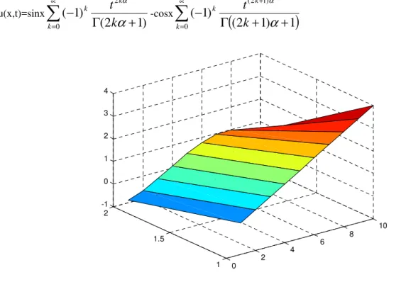
Fig 6. The surface shows the solution u(x,t) for Eq.(52) at α=1 and t=0.5

0 2

4 6

8 10

1 1.5

(10)

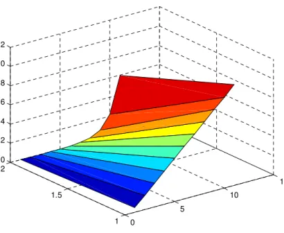
Fig.7 The surface shows the solution u(x,t) for Eq.(52) at α=1 and t=1.5 Example 6. Consider the space fractional advection-dispersion equation

0 ,

5 .

0

5 .

0 <

<

>

∂

+

∂

=

∂

t

x

u

x

u

t

u

π

β β α

α

(60)

)

2 cosh(

)

0 ,

(

x

u

=

(61)

[

]

β

α

_φ

φ

x

q

t

x

q

t

x

t

q

t

x

q

t

x

N

∂

−

∂

−

∂

=

(

,

;

)

0 .

5 (

,

;

)

0 .

5 (

,

;

)

;

,

(

[

]

t

q

t

x

q

t

x

L

∂

=

(

,

;

)

;

,

(

φ

L(c1(x))=0 (64)

[

_m₋₁

]

=

m

U

R

_β

β

α

_φ

φ

x

q

t

x

q

t

x

t

q

t

x

∂

−

∂

−

∂

(

,

;

)

5 .

0 )

;

,

(

5 .

0 )

;

,

(

[

(

,

)

(

)

]

)

,

(

)

,

(

₁ 1 ₁

1 −

− −

−

=

m m

+

m m

m

x

t

U

x

t

L

hH

r

t

R

U

u

χ

(66) Since m≥1, χm=1 and under the rule of solution expression suggested by Liao [16] we set the auxiliary function

H(r,t)=1 and we take h=-1 and we obtain the following successive approximations as

)

2 cosh(

)

,

(

0

x

t

x

u

=

(

)

(

t

)

x

t

x

u

₁

(

,

)

=

cosh(

2 )

0 .

5

2

α

+

2

β

0 2

4 6

8 10

1 1.5

(11)

( )

(

)













+

=

2 2 2

2

0 .

5

2

1 )

2 cosh(

)

,

(

x

t

x

t

u

α β

……… The final solution is

( )

(

)













+

=



=

k k k

n k

t

k

x

t

x

u

0 .

5

2

α

2

β

!

1 )

2 cosh(

)

,

(

0

(67)

When α=1 and β=1 the exact solution is

u

(

x

,

t

)

=

cosh(

2 x

)

e

2t (68)

Fig.8 Comparison of solutions of Eq.(60) for some values of t and x=0.5

using 4th_{term HAM approximation with}_α_{=0.25(blue curve),}_α_{=0.5(green curve),}_α_{=0.75(red curve)}

Fig.9 The surface area shows u(x,t) for the Eq.(60) using fourth term approximation of HAM with α=0.5 for some values of x and t(x=t)

0 0.1 0.2 0.3 0.4 0.5 0.6 0.7 0.8 0.9 1 0

0.1 0.2 0.3 0.4 0.5 0.6 0.7

t

u

0 0.1 0.2 0.3

0.4 0.5 0.6 0.7

0.8 0.9 1

0 0.1 0.2 0.3 0.4 0.5 0.6 0.7 0.8 0.9 1 0 0.1 0.2 0.3 0.4 0.5 0.6 0.7

0 0.1 0.2 0.3

0.4 0.5 0.6 0.7

0.8 0.9 1

(12)

Fig.11 The surface area shows u(x,t) for the Eq.(60) with α=1 for some values of x and t (x=t) Example. 7 Consider the space and time fractional diffusion equation

_∂

,

>

0 ,

0 <

≤

1 ,

1 ≤

≤

2 ∂

=

∂

β

α

β β α

α

t

x

u

c

t

u

(69) Here we take c=2

with initial condition

u

(

x

,

0 )

=

cos

(

2 π

x

)

,

x

∈

R

(70)

[

φ

]

α

φ

_α β

φ

_β

x

q

t

x

c

t

q

t

x

q

t

x

N

∂

−

∂

=

(

,

;

)

(

,

;

)

;

,

(

(71)

and linear operator

[

φ

]

α

φ

_α

t

q

t

x

q

t

x

L

∂

=

(

,

;

)

;

,

(

L(c1(x))=0 (73)

[

m−1

]

=

m

U

R

β

α

_φ

x

q

t

x

c

t

q

t

x

∂

−

∂

(

,

;

)

(

,

;

)

[

(

,

)

(

)

]

)

,

(

)

,

(

₁ 1 ₁

1 −

− −

−

=

m m

+

m m

m

x

t

U

x

t

L

hH

r

t

R

U

u

χ

(75) Since m≥1, χm=1 and under the rule of solution expression suggested by Liao [16] we set the auxiliary function

H(r,t)=1 and we take h=-1 and also this equation has sub diffusive behavior we obtain the following successive approximations as

)

2 cos(

)

0 ,

(

0

x

u

=

π

0 0.1 0.2 0.3

0.4 0.5 0.6 0.7

0.8 0.9 1

(13)

( )

(

)

α β

α

πβ

π

t

x

t

x

u

1

2

2 cos

2

2 )

,

(

1

+

Γ













+

=

( )

(

)

α β

α

πβ

π

2 2

2

1

2

2 cos

2

2 )

,

(

t

x

t

x

u

+

Γ













+

=

( )

(

)

α β

α

πβ

π

3 3

3

1

3

2

3

2 cos

2

2 )

,

(

t

x

t

x

u

+

Γ













+

=

………

The final solution is

( )

(

)



=

Γ

+













+

=

n k

k k

k

t

k

x

t

x

u

0

1

2

2 cos

2

2 )

,

(

α

β

α

πβ

π

(76)

When α=1, we get the closed form as

u

(

x

,

t

)

=

e

−8π2t

cos(

2 π

x

)

(77)

0 0.1

0.2 0.3 0.4

0.5 0.6

0.7 0.8 0.9

1

0 0.1 0.2 0.3 0.4 0.5 0.6 0.7 0.8 0.9 1 -200 -150 -100 -50 0 50 100 150 200

0 0.1 0.2

0.3 0.4

0.5 0.6 0.7

0.8 0.9

1

(14)

Fig.14 The surface area shows u(x,t) for the Eq.(69) with α=1 in Eq.(51) for some values of x and t (x=t) Example: 8 Consider the space and time fractional diffusion equation

_∂

,

>

0 ,

0 <

≤

1 ,

1 ≤

≤

2 ∂

=

∂

β

α

β β α

α

t

x

u

c

t

u

(78) Here we take c=1

With initial condition

u

(

x

,

0 )

=

x

3

−

x

2

,

x

∈

R

(79) We will apply the Liao’s method to solve Eq.(78) subject to the initial condition Eq.(79)

[

]

β

α

_φ

φ

x

q

t

x

c

t

q

t

x

q

t

x

N

∂

−

∂

=

(

,

;

)

(

,

;

)

;

,

(

(80)

and linear operator

[

φ

]

α

φ

_α

t

q

t

x

q

t

x

L

∂

=

(

,

;

)

;

,

(

L(c1(x))=0 (82)

[

_m₋₁

]

=

m

U

R

β

α

_φ

x

q

t

x

c

t

q

t

x

∂

−

∂

(

,

;

)

(

,

;

)

[

(

,

)

(

)

]

)

,

(

)

,

(

₁ 1 ₁

1 −

− −

−

=

m m

+

m m

m

x

t

U

x

t

L

hH

r

t

R

U

u

χ

(84)

H(r,t)=1 and we take h=-1 and also this equation has sub diffusive behavior we obtain the following successive approximations as

2 3 0

(

x

,

0 )

x

u

=

−

(

)

(

3 )

(

1 )

2

4

6 )

,

(

2 3

1

+

Γ













−

Γ

−

Γ

=

− −

α

β

α β

β

t

x

t

x

u

0 0.1 0.2

0.3 0.4 0.5 0.6

0.7 0.8 0.9

1

(15)

(

)

(

)

(

)

3 2 2 2 2

2

6

2 ( , )

4 2

3 2

2

1 x

x

t

u x t

β β α

β

α

− −





=



_

−



_

Γ

−

Γ

−

Γ

+





The final solution is

(

)

(

3 ) (

1 )

2

4

6 )

,

(

0

2 3

+

Γ













−

Γ

−

Γ

=



=

− −

α

β

α β

β

k

t

k

x

k

x

t

x

u

k n

k

k k

(85)

All the numerical experiments presented in this section were computed in double precision with some MATLAB codes on a personal computer System Vostro 1400 Processor x86 Family 6 Model 15 Stepping 13 Genuine Intel ~1596 Mhz

IV.CONCLUSION

In this paper, the homotopy analysis method (HAM) has been successfully applied to obtain the approximate/analytical solutions of the space and time fractional reaction-diffusion equations. This work shows that HAM has significant advantages over the existing techniques. It avoids the need for calculating the Adomian polynomials which can be difficult in some cases. The reliability of the method and reduction in the size of computational domain give this method wider applicability. The results show that HAM is a powerful mathematical tool for finding the exact and approximate solutions of the nonlinear fractional RDEs.

ACKNOWLEDGMENT

I am very grateful to the reviewers for their useful comments that led to improvement of my manuscript. REFERENCES

[1] R.Hilfer, Applications of Fractional Calculus in Physics, Academic Press, Orlando 1999.

[2] S. Das, Analytical solution of a fractional diffusion equation by variational iteration method, Computers Math. Appl. 57 (2009) 483-487.

[3] Z.Odibat, S.Momani, Application of variational iteration method to nonlinear differential equations of fractional order, Int. J. Nonlinear Sci. Numer. Simul. 7(1) (2006) 15-27.

[4] H.Xu, S.Liao, X.You, Analysis of nonlinear fractional partial differential equations with the homotopy analysis method, Commun. Nonlinear Sci. Numer. Simul. 14(4) (2009) 1152-1156.

[5] B.J.West, M. Bolognab, P. Grigolini, Physics of Fractal Operators, Springer, New York, 2003.

[6] K.S. Miller, B. Ross, An Introduction to the Fractional Calculus and Fractional Differential Equations, Wiley, New York, 1993. [7] S. Kumar, A. Yildirim,Yasir Khan, L. Wei, A fractional model of the diffusion equation and its analytical solution using Laplace

transform, Scientia Iranica, 19(4), (2012)1117-1123.

[8] H. Jafari, S. Seifi, Homotopy analysis method for solving linear and nonlinear fractional diffusion-wave equation, Commun Nonlinear Sci Numer Simulat 14 (2009) 2006–2012.

[9] Najeeb Alam Khan , Nasir-Uddin Khan , Asmat Ara , Muhammad Jamil , Approximate analytical solutions of fractional reaction-diffusion equations, Journal of King Saud University Science,24 (2012)111–118.

[10] Vipul K. Baranwal , Ram K. Pandey , Manoj P. Tripathi , Om P. Singh, An analytic algorithm for time fractional nonlinear reaction– diffusion equation based on a new iterative method, Commun Nonlinear Sci Numer Simulat 17 (2012) 3906–3921.

[11] S. Saha Ray, K.S. Chaudhuri, R.K. Bera, Application of modified decomposition method for the analytical solution of space fractional diffusion equation,Applied Mathematics and Computation,196(1) (2008) 294-302.

[12] Veyis Turut, Nuran Guzel, Comparing Numerical Methods for Solving Time-Fractional Reaction-Diffusion Equations, ISRN Mathematical Analysis, Vol.2012, Article ID 737206, doi:10.5402/2012/737206.

[13] G.Hariharan, K.Kannan, Haar wavelet method for solving Fisher’s equation, Appl.Math.Comput. 211 (2009) 284-292. [14] G.Hariharan, K.Kannan, Haar wavelet method for solving nonlinear parabolic equations, J.Math.Chem. 48 (2010) 1044-1061. [15] G.Hariharan, K.Kannan, A Comparative Study of a Haar Wavelet Method and a Restrictive Taylor's Series Method for Solving

Convection-diffusion Equations, Int. J. Comput. Methods in Engineering Science and Mechanics, 11: 4, (2010)173 - 184. [16] S.J.Liao, Beyond Perturbation: Introduction to Homotopy Analysis Method. CRC Press/Chapman and Hall, Boca Raton. (2004)

[17] G.Hariharan, The homotopy analysis method applied to the Kolmogorov–Petrovskii–Piskunov (KPP) and fractional KPP equations, J Math Chem (2013) 51:992–1000. DOI 10.1007/s10910-012-0132-5

[18] S.J.Liao, Comparision between the Homotopy analysis method and Homotopy perturbation method, Appl.math.comput. 169 (2005) 118-164.

[19] S.J.Liao, Notes on Homotopy analysis method:Some definitions and theorems, Commun Nonlinear sci.Numer.Simul,14 (2009) 983-997.

[20] S.J.Liao, On the Homotopy analysis method for non linear problems, Appl. Math. Comput, 147 (2004) 499-513.