Volume 2015, Issue 2, Year 2015 Article ID jiasc-00085, 16 Pages doi:10.5899/2015/jiasc-00085
Research Article
An analytic algorithm for the space-time fractional
reaction-diffusion equation
M. G. Brikaa∗
Department of mathematics Faculty of computers and informatics, Suez Canal University, Ismailia, Egypt
Copyright 2015 c⃝M. G. Brikaa. This is an open access article distributed under the Creative Commons Attribution License, which permits unrestricted use, distribution, and reproduction in any medium, provided the original work is properly cited.
Abstract
In this paper, we solve the space-time fractional reaction-diffusion equation by the fractional homotopy analysis method. Solutions of different examples of the reaction term will be computed and investigated. The approximation solutions of the studied models will be put in the form of convergent series to be easily computed and simulated. Comparison with the approximation solution of the classical case of the studied modeled with their approximation errors will also be studied.
Keywords:Space-time-fractional, Reaction-diffusion equation, Homotopy analysis.
1 Introduction
Nonlinear phenomena occur in a wide range of apparently different contexts in nature, for instance biological, eco-nomical, chemical and physical systems. Some of them can be described by nonlinear partial differential equations. A particular class of partial differential equations (PDE) is those modeling nonlinear reaction and diffusion phenomena [1, 2]. Nonlinear diffusion equations are important class of parabolic equations appearing in many physical problems like phase transition in mechanical, electrical and electronic engineering, biochemistry and dynamics of biological sciences and in many methods for image processing and computer vision [3, 4, 5]. Reaction diffusion equations are applied to describe numerous problems such as the CO oxidation on Pt(110) [6], the study ofCa2+waves on Xenopus oocytes [7], the study of re-entry in heart tissues [8, 9]. In [10] the linear Convection Diffusion (CD) equation was solved with the homotopy analysis method (HAM).
Transports of molecular oxygen from the blood plasma to the living tissue of the skeletal muscle or brain among capil-lary walls are very important topics in the medical field. The study of chemical reaction taking place the environment conditions or the living organisms are popular chemical problems. The spreading of an advantageous gene and the spatial temporal evolution of a population of individuals wich diffuses with a constant of diffusion or even according to a function and then grow according to a specific rule, are very important rules in biology [11, 12]. Similar types of propagation phenomena are widely occur in nature, especially in biology, chemistry and physics, see [13, 14, 15]. The nonlinear reaction diffusion equation of the characteristic Cauchy type has successfully manged to model such problems, namely,
∂u(x,t)
∂t = D
∂2u(x,t)
∂x2 +F(u), x∈R, t>0, (1.1)
u(x,0) = g(x)
whereu(x,t)is the concentration,F(u) =r(x,t)u(x,t)is the reaction parameter andD>0 is the diffusion coefficient. This equation has originally introduced by Fisher [12], and A. N. Kolmogrov, I. Petrovskii and N. Piskunov [11], to describe the evolution of the diffusion and the grow of population in a certain colony taking into consideration the conditions of the environments. Equation (1.1) has successfully modeled the reaction diffusion processes taking place in moving media such as fluids, atmosphere, chemistry, and ecology. Even the passive scalars substances which are simply transported by the flow can be modeled by equation (1.1).
In this paper, we consider a generalization of equation (1.1), we replace the space and time of equation (1.1) by fractional derivatives operators in the Caputo fractional derivative, namely
∂αu(x,t) ∂tα =D
∂βu(x,t)
∂xβ +F(u), x∈R, 0<α≤1, 1<β≤2, t>0, (1.2)
subject to the initial conditions:
u(x,0) =g(x) (1.3)
whereu(x,t)is the concentration,F(u) =r(x,t)u(x,t)is the reaction parameter andD>0 is the diffusion coefficient,
αandβ are a parameter describing the order of the fractional derivative. Four problems will be solved with different
r(x,t). For solving equation (1.2) we use the fractional homotopy analysis method (FHAM), to study the effect of the fractional ordersαandβon the analytical and approximation solutions of equation (1.2). The homotopy analysis method is used in [18] to solve equation (1.2) for differentr(x,t)but for the classical case asα=1,β=2.Our main aim is to find the approximation solutions of equation (1.2) for differentr(x,t)and compare the simulated solutions by the approximation solutions of the classical case. The approximation errors will also simulated for differentr(x,t), αandβ.
The organization of this paper is as follows. Section 2, is devoted to present some necessary definition and preliminary. The idea of the fractional homotopy analysis method (FHAM) is given in Section 3. In Section 4, applications of the fractional homotopy analysis method (FHAM) for the space-time fractional reaction-diffusion equation and numerical results are given. Finally, we give a summary to explain our results.
2 Basic Definitions of Fractional Calculus
In this section, we give some basic definitions and properties of the fractional calculus theory which are used further in this paper [16].
Definition 2.1. A real function f(x),x>0,is said to be in a space Cµ,µ∈R,if there exists a real number p(>µ)
such that f(x) =xpf1(x)where f1(x)∈C[o,∞),and it said to be the space Cµmif f(m)∈Cµ,m∈N.
Definition 2.2. The Riemann-Liouville fractional integral operator of orderα ≥0, of a function f(x)∈Cµ, and
µ≥ −1is defined as
Jαf(x) = 1
Γ(α)
∫ t
0 (
x−t)α−1f(t) dt, α>0, x>0 (2.4)
J0f(x) =f(x) (2.5)
Definition 2.3. For m to be the smallest integer that exceedsα, Caputo time fractional derivative operator of order
α>0is defined as
Dtαu(x,t) =∂ αu(x,t)
∂tα =
{ 1
Γ(m−α)
∫t
0(t−ı)
m−α−1∂mu(x,ı)
∂tm dı, f or m−1<α<m
∂mu(x,t)
∂tm , f or α=m∈N
(2.7)
Definition 2.4. The fractional derivative of f(x)in the Caputo sense is defined as
Dαf(x) =Jm−αDmf(t) = 1
Γ(m−α)
∫ x
0 (
x−t)m−α−1f(m)(t) dt (2.8) form−1<α≤m,m∈N,x>0,f ∈C−m1.
From Eq.(2.8), we get the following result
Dα(x−a)γ=
{ Γ(γ+1)
Γ(γ−α+1)(x−a)
γ−α
, f or α≤γ
0, f or α>γ (2.9)
3 Basic idea of the homotopy analysis method (HAM)
Here we give a brief description of the the HAM [17] to handle the general nonlinear problem,
NFD(u(x,t)) =0 (3.10)
whereNFDis a nonlinear fractional partial differential operator,xandtdenote independent variables andu(x,t)is an unknown function. For simplicity, we ignore all boundary or initial conditions, which can be treated in the same way. Based on the constructed zero-order deformation equation by Liao [17], we give the following zero-order deformation equation in the similar way
(1−q)L[v(x,t,q)−u0(x,t)] =qhNFD(v(x,t,q)), (3.11) whereq∈[0,1]is an embedding parameter,his a nonzero auxiliary parameter, andv(x,t;q)is an unknown function.
v(x,t;q)is related tou(x,t)as
v(x,t,0) =u0(x,t), v(x,t,1) =u(x,t) (3.12)
whereu0(x,t)is an initial guess ofu(x,t)
By expandingv(x,t;q)in Taylor series with respect toq, one has
v(x,t,q) =u0(x,t) + ∞
∑
m=1
um(x,t)qm, (3.13)
where
um(x,t) =
1
m!
∂mv(x,t,q)
∂qm |q=0, (3.14)
If the auxiliary linear non-integer order operator, the initial guess, and the auxiliary parameterhare so properly chosen, the series (3.13), converges atq=1. Hence we have
u(x,t) =u0(x,t) + ∞
∑
m=1
um(x,t), (3.15)
which is used mostly in the homotopy perturbation method (HPM). By this choice the HPM is considered as a special case of the HAM. According to Eq.(3.13), the governing equation can be deduced from the zero-order deformation (3.11). To do so, define the vector
→
un(x,t) ={u0(x,t),u1(x,t)...,un(x,t)} (3.17)
Differentiating Eq.(3.11), m times with respect to the embedding parameterq and then settingq=0 and finally dividing them bym!, we have the so-called mth-order deformation equation
L[um(x,t)−xmum−1(x,t)] =hNFR ( →
um−1(x,t) )
, (3.18)
where
NFR(um→−1(x,t) )
= 1
(m−1)!
∂m−1NFD(→v(x,t,q))
∂qm−1 |q=0, (3.19)
and
xm=
{
0,m≤1,
1,m>1. (3.20)
Finally, for the purpose of computation, we will approximate the HAM solution (3.15) by the following truncated series:
Qm= m−1
∑
k=0
uk(x,t) (3.21)
The mth-order deformation (3.18), is linear and thus can be easily solved, especially by means of a symbolic compu-tation software such as Mathematica, Maple, Matlab, and so on.
4 Application
Example 4.1. In this example, the solution of equation(1.2)is given for r(x,t) =constant=−1.That means we solve
Dαt u(x,t) =∂ βu(x,t)
∂xβ −u(x,t), x∈R, 0<α≤1, 1<β≤2, t>0, (4.22) with the initial condition
u(x,0) =e−x+x (4.23)
From Eqs.(3.17)and(3.18), we have the mth-order deformation equation as
um(x,t) =xmum−1(x,t) +hJtα
[
Dtαum−1(x,t)−
∂βum−1(x,t)
∂xβ +um−1(x,t) ]
(4.24)
From Eqs.(4.23)and(4.24), we have
u0(x,t) =e−x+x
u1(x,t) = x1u0(x,t) +hJtα
[
Dtαu0(x,t)−
∂βu0(x,t)
∂xβ +u0(x,t) ]
= h t
α
Γ(α+1) [
− ∞
∑
[β](−1)nxn−β
Γ(n+1−β)+x+e −x
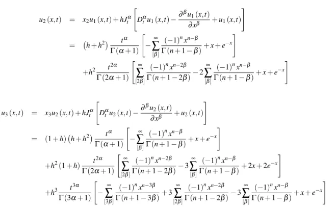
u2(x,t) = x2u1(x,t) +hJtα
[
Dαtu1(x,t)−
∂βu1(x,t)
∂xβ +u1(x,t) ]
= (
h+h2) t α
Γ(α+1) [
− ∞
∑
[β](−1)nxn−β
Γ(n+1−β)+x+e −x
]
+h2 t 2α
Γ(2α+1) [∞
∑
[2β](−1)nxn−2β
Γ(n+1−2β)−2 ∞
∑
[β](−1)nxn−β
Γ(n+1−β)+x+e −x
]
u3(x,t) = x3u2(x,t) +hJtα
[
Dαt u2(x,t)−
∂βu2(x,t)
∂xβ +u2(x,t) ]
= (1+h)(
h+h2) t α
Γ(α+1) [
− ∞
∑
[β](−1)nxn−β
Γ(n+1−β)+x+e −x
]
+h2(1+h) t 2α
Γ(2α+1) [∞
∑
[2β](−1)nxn−2β
Γ(n+1−2β)−3 ∞
∑
[β](−1)nxn−β
Γ(n+1−β)+2x+2e −x
]
+h3 t 3α
Γ(3α+1) [
− ∞
∑
[3β](−1)nxn−3β
Γ(n+1−3β)+3 ∞
∑
[2β](−1)nxn−2β
Γ(n+1−2β)−3 ∞
∑
[β](−1)nxn−β
Γ(n+1−β)+x+e −x
]
where[x]denotes the ceiling function and is equal to smallest integer greater than or equal to x.
Similarly, we get the next iterations and truncating the series(3.15) by the aid of mathematica, the approximate solution of Eq.(4.22)for m=6is written as
∼
u6(x,t) =u0(x,t) + 6
∑
m=1 um(x,t)
Note that the approximate solution∼um(x,t)converges to the exact solution e−x+xe−t, as m→∞for h=−1,α=1
andβ=2, since for these values of h,α andβ, the various um(x,t)are given by
u0(x,t) = e−x+x u1(x,t) = −xt u2(x,t) =
1 2xt
2 .. .
Hence, the exact solution is
u(x,t) =u0(x,t) + ∞
∑
m=1
um(x,t) =e−x+x
( 1−t+t
2
2!−
t3
3!+... )
=e−x+xe−t
which is same as the results obtained from [18, 19, 20, 21, 22] forα=1andβ=2.
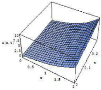
Figure 1: the approximate solution
Figure 2: the absolute error
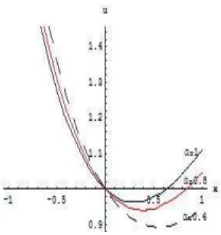
Figure 3: the approximate solution for differentβatx=3
Figure 5: the approximate solution for differentα atx=6
Figure 6: the approximate solution for differentα att=0.3
Example 4.2. Again we solve Eq.(1.2), but with r(x,t) =r(t) =2t,i. e.
Dαt u(x,t) =∂
βu(x,t)
∂xβ +2tu(x,t), x∈R, 0<α≤1, 1<β≤2, t>0, (4.25) with the initial condition
u(x,0) =ex (4.26)
From Eqs.(3.17)and(3.18), we have the mth-order deformation equation as
um(x,t) =xmum−1(x,t) +hJtα [
Dtαum−1(x,t)−∂ βu
m−1(x,t)
∂xβ −2tum−1(x,t) ]
(4.27)
From Eqs.(4.26)and(4.27), we have
u0(x,t) =ex
u1(x,t) = x1u0(x,t) +hJtα
[
Dtαu0(x,t)−
∂βu 0(x,t)
∂xβ −2tu0(x,t) ]
= −h t
α
Γ(α+1) ∞
∑
[β]xn−β
Γ(n+1−β)−2he
x tα+1
u2(x,t) = x2u1(x,t) +hJtα
[
Dαt u1(x,t)−
∂βu1(x,t)
∂xβ −2tu1(x,t) ]
= −h(1+h) [
tα
Γ(α+1) ∞
∑
[β]xn−β
Γ(n+1−β)+2 tα+1
Γ(α+2)e
x
]
+h2 t 2α
Γ(2α+1) ∞
∑
[2β]xn−2β
Γ(n+1−2β)+2h
2 t2α+1
Γ(2α+2) ∞
∑
[β]xn−β
Γ(n+1−β)(2+α)
+4h2(α+2) t 2α+2
Γ(2α+3)e
x
.
u3(x,t) = x3u2(x,t) +hJtα
[
Dtαu2(x,t)−
∂βu 2(x,t)
∂xβ −2tu2(x,t) ]
= −h(1+h)2 t α
Γ(α+1) ∞
∑
[β]xn−β
Γ(n+1−β)−2h(1+h)
2 tα+1
Γ(α+2)e
x
+2h2(1+h) t 2α
Γ(2α+1) ∞
∑
[2β]xn−2β
Γ(n+1−2β)
+2h2(1+h) t 2α+1
Γ(2α+2) ∞
∑
[β]xn−β
Γ(n+1−β)(4+α)
+8h2(1+h) (α+2) t 2α+2
Γ(2α+3)e
x.−h3 t3α
Γ(3α+1) ∞
∑
[3β]xn−3β
Γ(n+1−3β)
−2h3 t 3α+1
Γ(3α+2) ∞
∑
[2β]xn−2β
Γ(n+1−2β)(3+3α)
−4h3 t 3α+2
Γ(3α+3) ∞
∑
[β]xn−β
Γ(n+1−β)(3α+4+ (α+1) (2α+2))
−8h3(α+2) (2α+3) t 3α+3
Γ(3α+4)e
x
Similarly, we get next iterations and truncating the series(3.15)at m=5, we obtain an approximate solution of Eq.(4.25)as
∼
u5(x,t) =u0(x,t) + 5
∑
m=1 um(x,t)
Note that the approximate solution∼um(x,t)converges to the exact solution ex+t+t
2
, as m→∞for h=−1,α=1and
β=2, since for these values of h,αandβ, the various um(x,t)are given by
u0(x,t) = ex u1(x,t) = ex(t+t2) u2(x,t) = ex
(t2
2 +t
3+t4
2 )
Hence, the exact solution is
u(x,t) =u0(x,t) + ∞
∑
m=1
um(x,t) =ex
(
1+t+3t 2
2! + 7t3
3! +... )
=ex+t+t2
which is same as the results obtained from [18, 19, 20, 21, 22] forα=1andβ=2.
Fig. 7 shows the approximate solution∼u5for Eq.(4.25)when h=−1,α=1andβ=2, Fig. 8 shows the absolute error E6(h),Figs. 9 and 10 show the approximate solution
∼
u5for differentβ and Figs. 11 and 12 show the approximate solution∼u5for differentα.
Figure 7: the approximate solution
Figure 8: the absolute error
Figure 10: the approximate solution for differentβ att=0.2
Figure 11: the approximate solution for differentαatx=4
Figure 12: the approximate solution for differentαatt=0.4
Example 4.3. Consider the following space fractional reaction-diffusion equations(1.2)with r(x,t) =r(x) =−1−
4x2, namely
∂u(x,t) ∂t =D
2β
x u(x,t) + (−1−4x2)u(x,t), x∈R 0<β ≤1, t>0, (4.28)
with the initial condition
u(0,t) =et (4.29)
From Eqs.(3.17)and(3.18), we have the mth-order deformation equation as
um(x,t) =xmum−1(x,t) +hJx2β
[
D2βx um−1(x,t)−∂um−1(x,t)
∂t + (−1−4x 2)u
m−1(x,t)
]
(4.30)
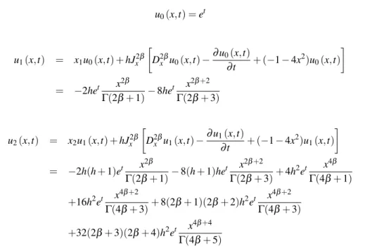
u0(x,t) =et
u1(x,t) = x1u0(x,t) +hJx2β
[
D2βx u0(x,t)−
∂u0(x,t)
∂t + (−1−4x 2)u
0(x,t) ]
= −2het x 2β
Γ(2β+1)−8he
t x2β+2
Γ(2β+3)
u2(x,t) = x2u1(x,t) +hJx2β
[
D2βx u1(x,t)−
∂u1(x,t)
∂t + (−1−4x 2)u
1(x,t) ]
= −2h(h+1)et x 2β
Γ(2β+1)−8(h+1)he
t x2β+2
Γ(2β+3)+4h
2et x4β
Γ(4β+1)
+16h2et x 4β+2
Γ(4β+3)+8(2β+1)(2β+2)h
2et x4β+2
Γ(4β+3)
+32(2β+3)(2β+4)h2et x 4β+4
Γ(4β+5)
Similarly, we get other iterations and truncating the series(3.15)at m=4, we obtain an approximate solution of Eq.(4.28)as
u(x,t) =u0(x,t) + 4
∑
m=1 um(x,t)
Note that the approximate solution∼um(x,t)converges to the exact solution as m→∞for h=−1andβ =1
u(x,t) =u0(x,t) +
∞
∑
m=1
um(x,t) =et
(
1+x2+x 4
2... )
=ex2+t
as m→∞for h=−1andβ =1which is same as the results obtained from [18] and [19] forβ =1.
Fig. 13 shows the approximate solution∼u4for Eq.(4.28)when h=−1andβ =1, Fig. 14 shows the absolute error E6(h)and Figs. 15 and 16 show the approximate solution
∼
u4for differentβ.
Figure 14: the absolute error
Figure 15: the approximate solution for differentβ atx=7
Figure 16: the approximate solution for differentβ att=0.3
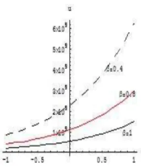
Example 4.4. Consider the following time fractional reaction-diffusion equations(1.2)when r=r(x,t) =4x2−2t+2
Dtαu(x,t) =∂ 2u(x,t)
∂x2 −(4x
2−2t+2)u(x,t), x∈R, 0<α≤1, t>0, (4.31) with the initial condition
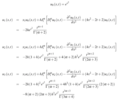
u(x,0) =ex2 (4.32)
From Eqs.(3.17)and(3.18), we have the mth-order deformation equation as
um(x,t) =xmum−1(x,t) +hJtα [
Dαt um−1(x,t)−∂ 2u
m−1(x,t) ∂x2 + (4x
2−
2t+2)um−1(x,t) ]
(4.33)
u0(x,t) =ex
2
u1(x,t) = x1u0(x,t) +hJtα [
Dαt u0(x,t)−∂ 2u
0(x,t)
∂x2 + (4x 2−
2t+2)u0(x,t) ]
= −2hex2 t α+1
Γ(α+2)
u2(x,t) = x2u1(x,t) +hJtα
[
Dαt u1(x,t)−
∂2u 1(x,t)
∂x2 + (4x 2−
2t+2)u1(x,t) ]
= −2h(1+h)ex2 t α+1
Γ(α+2)+4(α+2)h
2ex2 t2α+2
Γ(2α+3)
u3(x,t) = x3u2(x,t) +hJtα
[
Dαt u2(x,t)−
∂2u 2(x,t)
∂x2 + (4x
2−2t+2)u 2(x,t)
]
= −2h(1+h)2ex2 t α+1
Γ(α+2)+4h
2(1+h)ex2 t2α+2
Γ(2α+3)(2(α+2))
−8(α+2) (2α+3)h3ex2 t 3α+3
Γ(3α+4)
Similarly, we get next iterations and truncating the series(3.15)at m=6as
∼
u6(x,t) =u0(x,t) +
6
∑
m=1 um(x,t)
Note that the approximate solution∼um(x,t)converges to the exact solution ex
2+t2
, as m→∞for h=−1and α=1, since for these values of h andα, the various um(x,t)are given by
u0(x,t) = ex
2
u1(x,t) = ex
2
t2 u2(x,t) = ex2t
4
2!
.. .
Hence, the exact solution is
u(x,t) =u0(x,t) + ∞
∑
m=1
um(x,t) =ex
2(
1+t2+t 4
2!+... )
=ex2+t2
which is same as the results obtained from [18] and [19] forα=1.
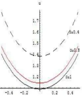
Fig. 17 shows the approximate solution∼u6for Eq.(4.31)when h=−1andα=1, Fig. 18 shows the absolute error E6(h)and Figs. 19 and 20 show the approximate solution
∼
Figure 17: the approximate solution
Figure 18: the absolute error
Figure 19: the approximate solution for differentαatx=6
5 Conclusion
The main interest of this paper is to use the FHAM to investigate the solution of the space–time fractional reaction-diffusion equation and to show its efficacy in contrast to the other reliable mathematical tools like the HPM and the VIM. Thus, it may be concluded that the HAM is a simple and a powerful analytical approach for handling fractional related PDEs. The results obtained from using the FHAM presented here agree well with the results obtained from [18] and [19].
References
[1] X. Y. Wang, Exact and explicit solitary wave solutions for the generalized Fisher equation, Phys Lett A, 131 (4/5) (1988) 277-283.
http://dx.doi.org/10.1016/0375-9601(88)90027-8
[2] A. M. Wazwaz, A. Gorguis, An analytical study of Fisher’s equation by using Adomian’s decomposition method, Appl Math Comput, 47 (2004) 609-620.
http://dx.doi.org/10.1016/S0096-3003(03)00738-0
[3] J. Weickert, Applications of nonlinear diffusion in image processing and computer vision, Acta Math Univ Comenianae, 70 (2001) 33-50.
[4] G. H. Cottet, L. Germain, Image processing through reaction combined with nonlinear diffusion, Math Comput, 61 (1993) 659-673.
http://dx.doi.org/10.1090/S0025-5718-1993-1195422-2
[5] A. Adamatzky, Costello BDL, Asai T, Reaction diffusion computers, Elsevier; (2005).
[6] M. Bar, N. Gottschalk, M. Eiswirth, G. Ertl, Spiral waves in a surface reaction: model calculations, J Chem Phys, 100 (1994) 1202-1212.
http://dx.doi.org/10.1063/1.466650
[7] J. P. Keener, Mathematical physiology, Interdisciplinary applied mathematics, New York: Springer; (1998).
http://dx.doi.org/10.1007/978-0-387-75847-3
[8] F. Fenton, E. Cherry, H. M. Hastings, S. J. Evans, Multiple mechanisms of spiral wave breakup in a model of cardiac electrical activity, Chaos, 12 (2002) 852-892.
http://dx.doi.org/10.1063/1.1504242
[9] V. Krinsky, A. Pumir, Models of defibrillation of cardiac tissue, Chaos, 8 (1998) 188-203.
http://dx.doi.org/10.1063/1.166297
[10] A. Fallahzadeh, K. Shakibi, A method to solve Convection-Diffusion equation based on homotopy analysis method, Journal of Interpolation and Approximation in Scientific Computing, 2015 (1) (2015) 1-8.
http://dx.doi.org/10.5899/2015/jiasc-00074
[11] A. N. Kolmogorov, I. Petrovskii, N. Piskunov, A study of the diffusion equation with increase in the amount of substance and its application to a biology problem, in selected work of A. N. Kolmogorov ed. V. M. Tikhomirov, Vol. I, P 242, Kluwer academic publishers, London (1991), original work Bull. Univ. Moscow, Ser. Int. A, 1,1 (1937).
[12] R. A. Fisher, The wave advance of advantageous genes, Ann. Eugenics, 7 (1937) 353.
http://dx.doi.org/10.1111/j.1469-1809.1937.tb02153.x
[13] J. D. Murray, Mathematical biology, New York: Springer; (2003).
[15] H. Wilhelmsson, E. Lazzaro, Reaction–diffusion problems in the physics of hot plasmas, Bristol and Philadel-phia: Institute of Physics Publications; (2001).
http://dx.doi.org/10.1887/0750306157
[16] A. A. Kilbas, H. M. Srivastava, J. J. Trujillo, Theory and Applications of Fractional Differential equations, Elsevier, (2006).
[17] S. J. Liao, Beyond Perturbation: Introduction to Homotopy Analysis Method, Chapman & Hall/CRC Press, Boca Raton, (2003).
http://dx.doi.org/10.4310/MAA.2003.v10.n2.a3
[18] A. S. Bataineh, M. S. M. Noorani, I. Hashim, The homotopy analysis method for Cauchy reaction-diffusion problems, Physics Letters A, 372 (2008) 613-618.
http://dx.doi.org/10.1016/j.physleta.2007.07.069
[19] Ahmet Yildirim, Application of He’s homotopy perturbation method for solving the Cauchy reaction diffusion problem, Computers and Mathematics with Applications, 57(2009) 612-618.
http://dx.doi.org/10.1016/j.camwa.2008.11.003
[20] R. K. Saxena, A. M. Mathai, H. J. Haubold, Computational solutions of unified fractional reactiondiffusion equations with composite fractional time derivative, Communications in Nonlinear Science and Numerical Sim-ulation, 27 (1) (2015) 1-11.
http://dx.doi.org/10.1016/j.cnsns.2015.02.021
[21] Alfonso Bueno-Orovio, David Kay, Kevin Burrage, Fourier spectral methods for fractional-in-space reaction-diffusion equations, BIT Numerical Mathematics, 54 (4) (2014) 937-954.
http://dx.doi.org/10.1007/s10543-014-0484-2
[22] Yuri Luchko, et al; Uniqueness and reconstruction of an unknown semilinear term in a time-fractional reaction-diffusion equation, Inverse Problems, 29 (6) (2013) 065019.