www.atmos-chem-phys.net/12/1031/2012/ doi:10.5194/acp-12-1031-2012
© Author(s) 2012. CC Attribution 3.0 License.
Chemistry
and Physics
The scale problem in quantifying aerosol indirect effects
A. McComiskey1,2and G. Feingold2
1Cooperative Institute for Research in Environmental Sciences, University of Colorado, Boulder, USA 2NOAA Earth System Research Laboratory, Boulder, USA
Correspondence to:A. McComiskey ([email protected])
Received: 10 September 2011 – Published in Atmos. Chem. Phys. Discuss.: 27 September 2011 Revised: 16 December 2011 – Accepted: 3 January 2012 – Published: 23 January 2012
Abstract. A wide range of estimates exists for the radia-tive forcing of the aerosol effect on cloud albedo. We argue that a component of this uncertainty derives from the use of a wide range of observational scales and platforms. Aerosol influences cloud properties at the microphysical scale, or the “process scale”, but observations are most often made of bulk properties over a wide range of resolutions, or “analysis scales”. We show that differences between process and anal-ysis scales incur biases in quantification of the albedo effect through the impact that data aggregation and computational approach have on statistical properties of the aerosol or cloud variable, and their covariance. Measures made within this range of scales are erroneously treated as equivalent, lead-ing to a large uncertainty in associated radiative forclead-ing esti-mates. Issues associated with the coarsening of observational resolution particular to quantifying the albedo effect are dis-cussed. Specifically, the omission of the constraint on cloud liquid water path and the separation in space of cloud and aerosol properties from passive, space-based remote sensors dampen the measured strength of the albedo effect. We ar-gue that, because of this lack of constraints, many of these values are in fact more representative of the full range of aerosol-cloud interactions and their associated feedbacks. Based on our understanding of these biases we propose a new observationally-based and process-model-constrained, method for estimating aerosol-cloud interactions that can be used for radiative forcing estimates as well as a better char-acterization of the uncertainties associated with those esti-mates.
1 Introduction
Boundary layer clouds have been identified as a major source of uncertainty in climate sensitivity and climate change (Bony and Dufresne, 2006; Medeiros et al., 2008). The in-fluence of aerosol particles on these clouds, via modification to microphysical processes, further contributes to this uncer-tainty. Aerosol has potentially substantial impacts on cloud radiative forcing (“aerosol indirect effects”), cloud-climate feedbacks, and water resources through changing patterns of precipitation; however, quantifying the associated mech-anisms and impacts through observation, and representing those processes in models, has proven to be extremely chal-lenging.
(e.g., Murphy et al., 2009). These tend to be at the low end of the range produced by GCMs.
Indirect effects related to cloud water variability and pre-cipitation that potentially affect cloud amount and lifetime, traditionally considered feedbacks, have an even more poorly quantified impact on the radiation budget (Quaas et al., 2009; Lohmann et al., 2010). The numerous process studies that have attempted to assess the magnitude of these effects have generated conflicting answers, and even the sign of the cloud water response to changes in the aerosol is in question (Al-brecht, 1989; Ackerman et al., 2004; Brenguier et al., 2003a; Matsui et al., 2006; Xue et al., 2008; Lebsock et al., 2008). While the focus of this study is on the albedo effect, many of the issues presented are relevant to indirect forcing in the broadest sense.
This paper will show that progress in narrowing the un-certainty range in the albedo effect has been hampered by neglect of important observational aspects of aerosol-cloud interaction metrics. First, obtaining direct, independent, and collocated measurements of each pertinent variable is diffi-cult, but required. Second, there is a range of observational scales or “analysis scales” to consider that are usually dif-ferent from the scale of the driving mechanism or “process scale”. Due to the effects of averaging on statistics, an anal-ysis at the process scale is not equivalent to that made at coarser scales, resulting in metrics that may be too high or too low. The most accurate representation of a process re-sults from an analysis in which the process scale and analy-sis scale are the same. Current analyses of the cloud-albedo effect span scales from the microphysical (the process scale) to the global (see references in Table 1). This spectrum of analyses has grown out of an interest to link important mi-crophysical processes with the resulting radiative impacts at larger, climatically relevant (meso-to-global) scales, but also contributes directly to uncertainty. Finally, aerosol and cloud properties, and thus aerosol-cloud interaction processes, are highly spatially distributed. Distributing metrics that are ei-ther too high or too low uniformly over space, as is often done in climate models, further biases global estimates of the effect, and increases uncertainty.
It is our assertion that disparities in scale among various physical processes, inconsistencies in scale and computa-tional approach among observations from various platforms, and disparities in the scales of representations (parameteriza-tions) in models are responsible for a large part of the con-fusion in estimating the magnitude of indirect effects. The challenge can be broadly posed as follows: how does one represent variable, yet potentially strong local processes at coarse scales? An assessment of the characteristic spatial variability of aerosol and cloud properties is required, as is a consideration of analysis scales that are representative of the process, yet still accessible to global studies. The primary goals of this paper are to identify key factors that contribute to the differences in the scale-dependent range of aerosol-cloud interaction metrics found in the literature and
charac-terize the physical meaning of this spectrum of results. An outcome of this work is a proposed methodology for deriv-ing an observationally-based and process-model-constrained estimate of radiative forcing that can be applied to different cloud regimes and aggregated up to the global scale.
2 Aggregation and scale biases in statistics
2.1 Current state of understanding aerosol-cloud interactions
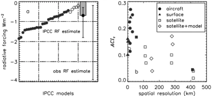
Among the aerosol indirect effects, the IPCC has to date es-timated the radiative forcing of the first indirect effect, or albedo effect (Twomey, 1974) only. This quantity has the largest uncertainty of all of the radiative forcings and is also the only estimate derived solely from model results. A break-down of the radiative forcing estimates by each of the IPCC Fourth Assessment Report (AR4) models is shown in Fig. 1a. The closed circles indicate models that represent the cloud-albedo effect through the use of drop activation parameteriza-tions and the open circles indicate models that use satellite-based empirical parameterizations. The models that apply empirical relationships between cloud and aerosol properties consistently predict the weakest radiative forcing. The latter are similar in magnitude to the purely satellite-based assess-ments such as those reported e.g., by Quaas et al. (2008), although these estimates are not included in AR4. Empirical estimates of aerosol-cloud interactions derive from a range of in situ airborne measurements, ground-based remote sensing, and space-based remote sensing of aerosol and cloud proper-ties. Twomey (1974) used airborne, process-scale measure-ments to show that an increase in cloud condensation nuclei from pollution would result in brighter clouds by increasing cloud optical depth, all else being equal. This approach re-quired the cloud water variable be constrained in order to assess the impact of the aerosol on cloud albedo while con-trolling for other impacts on the cloud albedo. To quantify the microphysical component of the albedo effect, Feingold et al. (2001) proposed a metric IE= −dlnre/dlnτa, where reis the cloud drop effective radius andτa, the aerosol opti-cal depth, holding cloud liquid water constant for all opti- calcula-tions. Later, the terminology for this calculation was changed to ACI (aerosol-cloud interactions) to clarify that the result represents not the indirect effect, which is a response of cloud albedo to aerosol, but instead the microphysical response of the albedo effect (McComiskey et al., 2009). Several other terminologies have been used in the literature, but for consis-tency ACI will be used throughout this work.
ACI has been reported or derived later from measurements published in the literature for almost two decades. A vari-ety of proxies has been used to represent the aerosol par-ticles affecting the cloud, including aerosol number concen-trationNa,τa, and aerosol index AI (the product ofτaand the
˚
Table 1.References used in Fig 1b. All studies address low or liquid clouds.
method/ parameters ACIτ resolution temporal L∗
instrument used averaging
Ground
Feingold et al. (2003) RS (remote sensing) 0.10 20 s yes
Garrett et al. (2004) RS+in situ 0.15 30 min yes
Kim et al. (2008) RS+in situ 0.15 5 min yes
Lihavainen et al. (2008) in situ 0.24 1 h yes
McComiskey et al. (2009) RS+in situ 0.16 20 s yes
Airborne
Twohy et al. (2005) in situ 0.27 10–60 min
Raga and Jonas (1993) in situ 0.09 NA no
Martin et al. (1994) in situ 0.25 30 km
Gultepe et al. (1996) in situ 0.22 ∼12 km yes
O’Dowd et al. (1999) in situ 0.20
McFarquhar and Heymsfield (2001) in situ 0.11
Ramanathan (2001) in situ 0.21–0.33
Lu et al. (2007) in situ 0.19 30 km
Lu et al. (2008) in situ 0.14 leg means
Satellite
Nakajima et al. (2001) AVHRR Nd;Na 0.17 0.5◦ 4 months
Bulgin et al. (2008) ASTER-2 re;τa 0.10–0.16 (0.13) 1◦ seasonal/3 months no Kaufman et al. (2005) MODIS re; AI 0.046–0.174 (0.0975) 1◦ simultaneous/daily no
Sekiguchi et al. (2003) AVHRR re;Na 0.1 2.5◦ daily no
Lebsock et al. (2008) MODIS re; AI 0.07 1 km to 1◦ simultaneous no Sekiguchi et al. (2003) POLDER re;Na 0.07 (ocean) 2.5◦ monthly no Quaas et al. (2006) MODIS Nd;τa 0.04 3.75◦×2.5◦ daily
Quaas et al. (2004) POLDER re; AI 0.04 (ocean)/0.012(land) 3.75◦×2.5◦ simultaneous no Satellite + Model
Breon et al. (2002) POLDER + back trajectories re;τa, AI 0.085 (ocean)/0.04 (land) 150 km 3 months no Chameides et al. (2002) ISCCP + CTM τc;τa 0.17 (all)/0.14 (low cloud) 280 km annual no
∗L-constraint used in calculation of ACI.
byα. Similarly, various proxies have been used to repre-sent the cloud response to the change in aerosol, e.g., cloud optical depthτc, cloud drop number concentrationNd, and re. Using data for which the analysis scale closely matched the process scale, McComiskey et al. (2009) showed empir-ically that there is consistency amongst calculations of ACI using different microphysical proxies, provided the appropri-ate constraint on cloud liquid wappropri-ater pathLis applied. Thus, ACIτ=
∂lnτc ∂lnα L
0<ACIτ<0.33 (1a)
ACIr= − ∂lnre ∂lnα L
0<ACIr<0.33 (1b)
ACIN= dlnNd
dlnα 0<ACIN<1 (1c)
ACIτ= −ACIr= 1
3ACIN. (1d)
Figure 1b presents a representative selection of ACIτ
val-ues (0≤ACI≤0.33) from the literature originating from a
Fig. 1. (a)Radiative forcing estimates by each IPCC model and the overall IPCC radiative forcing estimate in comparison to an ob-servational estimate for the cloud albedo effect resulting from the values in 1b. (b)Values from the literature quantifying the albedo effect using some variant of Eq. (1), expressed here as ACIτ, and
range of observational platforms. Closed symbols denote studies where calculations were constrained byLand open symbols denote studies for which this constraint was ignored. It is clear that quantification of the albedo effect is sensitive to scale and the constraint onL. The studies that occupy the coarsest resolutions on this plot were intentionally un-dertaken at resolutions that are comparable to GCM grid cell sizes in order to produce evaluation datasets or empirical pa-rameterizations for those models. The association between weak radiative forcing and these coarse-scale parameteriza-tions as opposed to stronger radiative forcing from both mi-crophysical scale observations and model schemes becomes evident.
Published ACI values span almost the entire physically meaningful range from 0 to 0.33 (see Table 1). Data types used as input to these calculations range from those in which the process and analysis scales are closely matched to those in which the analysis scales are highly aggregated relative to the process scale. This begs the question: to what extent are these values meaningful, and how might they be applied in GCMs?
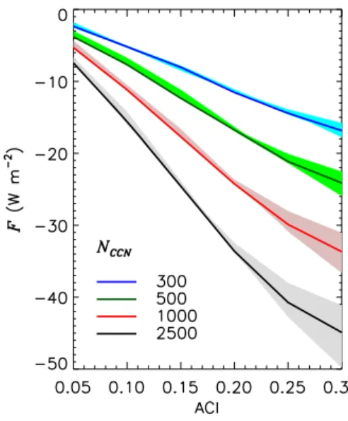
Observational estimates of forcing have been omitted in the overall radiative forcing estimate of the albedo effect in the IPCC AR4, so we perform rough calculations based on ACI values drawn from the literature. At the right of Fig. 1a, the overall IPCC radiative forcing (grey bar with range) is compared to a rough, 1-D (plane-parallel) calculation of what the range of forcing for the observations in Fig. 1b would be, following radiative transfer calculations in McComiskey and Feingold (2008). The calculations assume a factor of 3 in-crease in cloud condensation nucleus concentrationsNCCN (from 100 cm−3 to 300 cm−3)and a global average liquid water cloud cover of 25 % with meanL=125 g m−2. ACI is varied over nearly the entire range of observed values from Fig. 1b. The result is a range in forcing from −0.2 to−3.9 W m−2, much larger than the range estimated from GCMs. Figure 2 shows the variability in forcing as a func-tion of ACI for variousL and CCN perturbations for 1-D or plane-parallel conditions (100 % cloud cover). While this is a rudimentary estimate of the range of radiative forcing from observations with broad assumptions, it illustrates that observationally-based radiative forcing estimates of this kind are too variable to be useful in global observational analyses or model parameterizations.
If uncertainties in radiative forcing of aerosol indirect ef-fects are to be reduced, it is necessary to understand what drives the scale biases seen in Fig. 1, both in how they re-late to quantifying the albedo effect, and also in how they may reflect on analyses of all indirect effects including, for example, the impact of aerosol on cloud cover andL. In the following sections, we attempt to define the factors contribut-ing to these biases and provide some potential solutions that allow for a useable observationally-based estimate.
Fig. 2. The amount of forcing as ACIτ varies across the observed
range in Fig. 1b.Values for forcing are given for the difference of four differentNCCN concentrations fromNCCN=100 cm−3 and the shaded envelopes represent the range of forcing for each of these concentrations for a range ofLfrom 50–200 g m−2.
2.2 Scale and statistics
The concept of ecological fallacy gained much attention when Robinson (1950) illustrated that inferring characteris-tics of relationships among individuals from area-aggregated units did not produce reliable results. Since then, the dif-ficulty in producing reliable statistics from aggregated areal data has been a subject of much concern in fields such as ecology and geography. We will borrow from the field of ge-ography, where theModifiable Areal Unit Problem(MAUP) (Openshaw, 1984) has been used to describe the effect of level of aggregation (the scale problem) on uni- and multi-variate statistics.
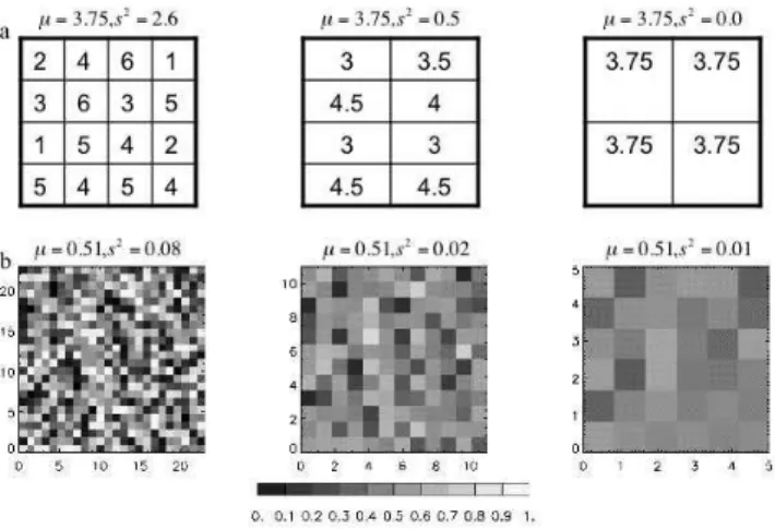
Fig. 3. Change in variances2 with aggregation of two simple datasets(a)from Jelinski and Wu (1996) and(b) randomly gen-erated numbers. Note the constant value for the meanµin each case as the variance decreases with aggregation.
scales in the literature (Fig. 1). Essential to understanding the effects of aggregation on metrics of aerosol-cloud inter-actions is an assessment of characteristic spatial variability of aerosol and cloud properties.
Anderson et al. (2003) quantified significant scales of vari-ability in aerosol amount on horizontal scales of 40–400 km and temporal scales of 2–48 h. For heterogeneous conditions such as smoke plumes near their source, Shinozuka and Re-demann (2011) found the relevant scale to be ∼1 km. At scales smaller than this, it might be safe to assume that the aerosol adjacent to clouds is a good proxy for that between the clouds (neglecting cloud contamination of the aerosol measurement). The range of 1–400 km is large, however, and spans the bulk of spatial scales used in studies of ACI (see Fig. 1b)
Typical cloud microphysical scales of variability are much smaller. Fast response instruments show variability in cloud properties down to cm scales (Brenguier, 1993; Gerber et al., 2001), but considering the scales of motion that drive convection, spatial scales of 10 m–100 m adequately capture bulk cloud properties. These small scales of variability are observable from in situ and ground-based measurements but typically not from space. Wood and Hartmann (2006), us-ing MODIS data at a base resolution of 1 km, found domi-nant scales ofLvariability to be between 5 and 50 km, still smaller than the typical analysis scales of≥1◦.
The radiative properties of clouds from various regimes contribute to variability dominant at scales of 5 km and be-low (e.g., Oreopoulos et al., 2000; Davis et al., 1997). For remote sensing of stratiform boundary layer clouds, the scale at which competing errors associated with the neglect of 3-D radiative transfer effects is minimized is 1 km (Zinner and Mayer, 2006). At scales smaller than 1 km, neglecting hori-zontal photon transfer (i.e., the independent pixel
approxima-tion) introduces error, while at scales>1 km, the plane par-allel assumption contributes progressively to error in the op-posite direction. Without discounting the potential for vari-ability in aerosol, cloud, and radiation to manifest at smaller scales, 1 km2may represent a reasonable and practical areal unit for study of the problem. This particular scale may hold only for stratiform clouds and is clearly problem-specific.
2.2.1 Scale and ACI calculations
Cloud responses to changes in aerosol are typically repre-sented by power-law functions. Using a linear regression be-tween aerosol and cloud propertiesy=a+bx, whereyis the logarithm of the cloud property (dependent variable) andxis the logarithm of the aerosol property (independent variable), ACI is simply an estimator of the regression slopeb, which can be defined as
ˆ b=rxy
sy
sx
or ACI=raerosol,cloud scloud saerosol
.
The correlation coefficient is rxy=
COV(x,y) sxsy
with COV(xy)the covariance between andxandyandsxthe
standard deviation ofnsamples of variablex with meanx¯. The standard deviation ofx, the square root of the variance sx2, is
sx= s
P
i (x− ¯x)2
n−1 .
Hence, changes in ACI with aggregation will be a function of the relative rate of change in the variance of each of the logarithms of aerosol and cloud properties employed, and in the change in covariance between the two. It will be shown that the rate of change ins2with aggregation or scale changes is dependent on the characteristics and the distributions of the properties of interest.
Numerous empirical studies addressing the MAUP have shown that increasing the level of aggregation results in a loss of variance, leading to an increase inrxy (Openshaw,
Sekiguchi et al. (2003) provide an example from AVHRR data that are successively averaged in space and time, show-ing that with aggregation, r increases rapidly (see their Fig. 2). They argue that more highly aggregated data pro-vide a better estimate of the effect due to a higher correlation. Whilerrepresents the goodness-of-fit of a linear regression model in this case, it cannot necessarily be used as an indica-tor of the optimal scale at which to analyze the relationship between aerosol and cloud. We will provide evidence that while disaggregated data may exhibit a wider spread, the fit to these data more accurately represents aerosol-cloud pro-cesses and thatrorr2should not be used as a criterion for determining the fitness of datasets for quantifying ACI or the albedo effect.
2.2.2 Measurements and ACI calculations
Measurement approach dictates whether data is disaggre-gated or aggredisaggre-gated and also the degree of aggregation. In any approach to observation, instrument resolution is depen-dent on limitations generated by integration time and sensor field-of-view. In the case of aerosol or cloud drop concen-tration, in situ data are generally disaggregated data, as the basic unit of measure is the particle. Temporal resolution is often maximized for in situ observations, within instrumental constraints, as the interest is typically on the microphysical scale. Ground-based and space-based remote sensing pro-duce aggregated data in the form of bulk properties (an av-erage measure of particles, e.g., cloud optical depth) with ground-based data having the potential for much finer reso-lution. Point-based remote sensing from the ground at high temporal resolution can capture changes in the microphysical and optical properties at a scale that resolves the processes of interest and thus may be considered a proxy for disaggre-gated data. For satellite-based sensors, the basic areal unit of study, the pixel, tends to be arbitrary relative to the process being studied, and is based rather on general optimization of the sensor. For each of these types of observation, the basic units of measure are “modifiable” through the use of statis-tical methods for upscaling or aggregation of the data. This is often the case with operational products where retrievals require some amount of averaging or with global coverage products that are much more reasonably distributed and ex-amined at coarser resolutions.
Progressively increasing the level of aggregation of data by averaging carries a number of consequences. The het-erogeneity in either the aerosol or cloud microphysical variable internal to the sampling unit is lost at coarser scales. Averaging to larger scales also progressively in-creases the likelihood of contribution of the multiple (liq-uid) cloud processes (activation, condensation, entrainment-mixing, collision-coalescence, sedimentation, scavenging), making it less and less relevant to the albedo effect. Thus, the quantification of ACI (constrained byL)from disaggre-gated data, regardless of their spread, will be more accurate
because measurements were made at the scale of the process and for well-defined conditions. Confidence in that measure should be evaluated by a statistical significance test (p-value) of the regression, regardless of the correlation coefficient, al-though the two are generally related.
While the use of disaggregated data provides the most ac-curate representation of the process, we wish to implement this knowledge at the global scale, for which the required fine resolution of either observations or models is not fea-sible, and for which the operational products from satellite sensors are convenient. Below, we provide some illustrations of the impact of scale on quantifying the albedo effect that address the above dilemma. If we are to exploit data over a wide range of scales, from in situ to global coverage using satellite-based sensors, an understanding of the associated errors is required. The following discussion is intended to illuminate the primary causes of those errors.
3 Methods
To illustrate the potential effects of aggregation on the statis-tical properties of data, we use a range of data sources over the northeast Pacific Ocean. Our data sources are associated with the marine stratocumulus cloud regime, and derive from the Dynamics and Chemistry of Marine Stratocumulus Phase II (DYCOMS-II) experiment (Stevens et al., 2003), which took place off the coast of southern California in July of 2001, as well as the Department of Energy (DOE) deploy-ment to the northern coast of California in 2005. We draw from cloud-resolving model output, ground-based in situ and remote sensing, and satellite-based remote sensing products of aerosol and cloud properties from the Moderate Reso-lution Imaging Spectroradiomenter (MODIS) sensor aboard the Terra satellite. A description of the various data sources and pertinent information follows.
3.1 Disaggregated data: Pt. Reyes surface observations
High-resolution surface observations are used as a proxy for disaggregated data as previously indicated. Measurements of aerosol and cloud properties are taken from the DOE deploy-ment of the Atmospheric Radiation Measuredeploy-ment (ARM) Mobile Facility to Pt. Reyes, CA that ran from March to September of 2005. Near-continuous in situ observations of aerosol and cloud properties as well as radiometer observa-tions ofLare available along with daytime observations of τc at a temporal resolution of 20 s. These data are used to produce daily, high temporal resolution correlation statistics between aerosol and cloud properties.
3.2 Aggregated data: MODIS
the California coast over the DYCOMS-II operating region and extend over a larger area of the northeast Pacific. We use Level 2 (L2) data, which provides instantaneous cloud properties at 1 km (Platnick et al., 2003) and aerosol proper-ties at 10 km resolution (Remer et al., 2005), as well as daily averaged Level 3 (L3) global coverage data at 1◦resolution.
3.3 Cloud-resolving model output
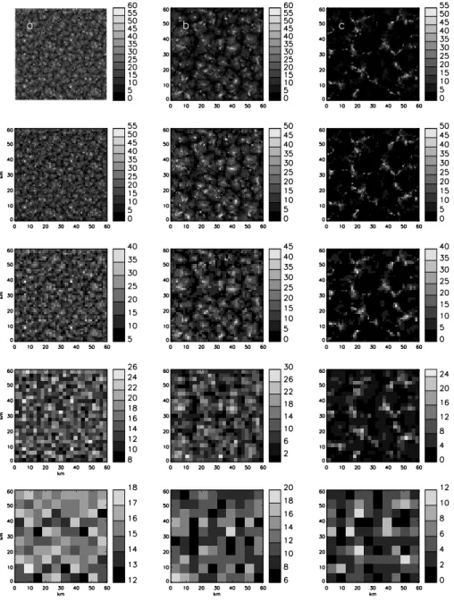
Model output is especially useful for exploring scale effects on quantifying aerosol-cloud interactions since, unlike most observations, co-located variables required for the calcula-tions are present in each grid cell and at each time step. We use model output from the Weather and Research Forecasting (WRF) model run in cloud-resolving mode (Wang and Fein-gold, 2009) to illustrate the effects of data aggregation on ACI. The WRF model was implemented using environmen-tal parameters from the DYCOMS-II experiment. Simula-tions were made on 300 m (horizontal)×30 m (vertical) grids over a 60×60 km domain with a time step of three seconds. Snapshots of model output are examined at 15 min intervals. Cloud optical depthτcfrom the native WRF runs are shown in the top row of Fig. 4. The three separate instances (a, b, and c) represent different aerosol concentrationsNaand tem-poral evolutionstas follows: (a)Na=500 cm−3,t=3 h, (b) Na=500 cm−3,t=6 h, (c)Na=150 cm−3,t=9 h. These different instances result in cloud fields in various stages of open and closed cell development with distinct patterns and distributions of cloud properties.
3.4 PDF sampling for ACI estimation
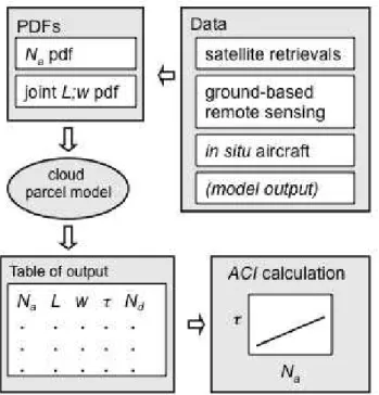
The WRF model simulations were all initialized with a con-stant Na across the domain so that they exhibit little spa-tial and temporal variability, except in strongly precipitating conditions. However, in order to calculate correlations be-tween cloud and aerosol properties, as well as ACI, a range of Na must be present. To achieve this, we ignore the Na used to generate the simulations and instead use a randomly generated normal distribution ofNa with a mean at the ini-tial modeledNa. Although aerosol number concentrations are often log-normally distributed (Asmi et al., 2011), a nor-mal distribution is used here to simplify illustration of our method. Next we build a jointLand updraft velocityw dis-tribution using the WRF output. Using a method of random sampling that provides a rigorous sample of the population of theNa and joint L; w probability distribution functions (PDF), each set ofNa,Landwis used as input to an adia-batic cloud parcel model (Feingold and Heymsfield, 1992) to produce a proxy data set forτc,Nd, andre. The model pro-duces physically consistent sets ofNa,L,Nd,re andτc that can be considered representative of co-located aerosol and cloud properties, constrained by the model physics and fre-quency distribution of the aerosol and cloud measurements. In the more general case, model physics can be adapted for
the cloud regime of interest by including entrainment mixing and other relevant processes. A flowchart representing this method is given in Fig. 5. Since the random generation of Na distributions and the sampling approach results in slight variations in the value of ACI with each separate realization, averages are taken to achieve a robust estimate of ACI. Each data point in an ACI calculation shown in this study is an average from a set ofn=30 realizations of the parcel model. This method of sampling data in conjunction with the use of a process-scale model provides a comprehensive data set of well distributed Na, L, and τc from which to calculate and explore the impacts of aggregation and other data con-straints on ACI. Note that application of this methodology does not preserve the originalτcPDF in the WRF simulations because a PDF ofNa has been applied to generate the PDF ofτc; nevertheless, averageτcand the shape of the distribu-tion is similar. This does not detract from the results since the illustrative nature of these exercises is key. We will apply this methodology in Sect. 4 and also explore extended ap-plications of this approach in semi-empirical quantifications and model parameterizations of the cloud-albedo effect, in Sect. 5.
4 Observational biases in ACI
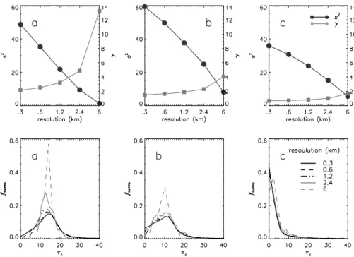
WRF model output is used to illustrate the basic effects of aggregation on statistics of cloud microphysical properties. Progressive aggregation of the WRF-derivedτc field from the original resolution of 0.3 km to 6 km (Fig. 4) results in changes in several basic statistical parameters. Note the dif-ferent scale bars and decrease in range (the difference be-tween maximum and minimum values ofτc)with each level of aggregation in Fig. 4. The scene s2, and τc probabil-ity distribution functions PDFs for each of these scenes are provided in Fig. 6. The homogeneity parameter γ=(µ/s)2 (Barker, 1996; Wood and Hartman, 2006), where µ is the mean andsis the standard deviation ofτc, is included in ad-dition tos2in reference to several other studies that use this parameter.
Fig. 4.Modeledτcfor three aerosol conditions and stages of temporal evolution:(a)Na=500 cm−3,t=3 h,(b)Na=500 cm−3,t=6 h, (c)Na=150 cm−3,t=9 h. The five levels of aggregation (rows) represent resolutions of 0.3, 0.6, 1.2, 2.4, and 6 km.
further aggregations. The change in these parameters is non-linear with scale and different for the three different cloud morphologies in accord with the scale of organization, i.e., characteristic length scales of the cloud features. The specific impacts of variation in organization and cloud field morphol-ogy on statistical parameters will be discussed further in the following section.
Figure 7 provides the correlation coefficient betweenNa andτcfrom the PDF sampling outlined in Fig. 5 for data from Fig. 4 and corresponding to the statistics in Fig. 6. The corre-lation coefficientrshows a dramatic increase with aggrega-tion as expected from previous discussions, with the amount
of increase varying with the correlation length scale of cloud features in each of the scenes from Fig. 4a, b, and c. Despite theoretical (Eq. 2) and empirical evidence that aggregation leads to an increase inrx,y, which would lead to an increase
Fig. 5. Flow chart of the random sampling method for an observationally-based approach to ACI calculations. PDFs for input to a process-scale model can be built from a variety of sources in-cluding model output and measurements made at a range of scales.
cloud properties in horizontal space in passive satellite re-mote sensing products and (2) the lack of constraint on L when performing ACI calculations. The latter will be ex-plored with WRF model output whereas the former requires analysis of ground-based and satellite remote sensing data to address the relevant spatial scales of separation.
4.1 Separation in horizontal space between aerosol and cloud properties
The problem of spatial separation between aerosol and cloud fields is particular to passive, satellite remote sensing. In the case of airborne field campaigns one can measure near-coincident in situ aerosol and cloud microphysical proper-ties (e.g., Twomey, 1974; Twohy et al., 2005 and references therein) or use stacked aircraft to assess the cloud albedo ef-fect by measuring reflectance in a single column (Brenguier et al., 2003b; Roberts et al., 2008). Measurements of aerosol-cloud interactions using ground-based remote sensing pro-vide high temporal resolution (order 20 s), co-located data for aerosol and cloud properties in a single column of air (e.g., Feingold et al., 2003; Kim et al., 2008) and improve confi-dence that the aerosol measured is that with the potential to impact the cloud properties measured. Ground-based remote sensing and airborne in situ samples are, however, limited in spatial coverage.
Space-based passive remote sensors provide a global per-spective of aerosol-cloud interactions, but co-located re-trievals of aerosol and cloud properties from these sensors are not physically possible. For the examination of aerosol-cloud interactions, an assumption is made that the aerosol is sufficiently homogeneous such that measurements made between clouds are representative of the aerosol feeding into the cloud from below. Even with this assumption, there is po-tential for aerosol measurements between clouds to be con-taminated by humidification, cloud fragments, and enhanced photon scattering (see e.g., discussion in Koren et al., 2009), although these issues are not addressed here. When sepa-rated in space or time, the relationship between the measured aerosol concentration and resulting cloud microphysics are likely less representative of the causal relationships that drive the albedo effect and that ACI is intended to quantify.
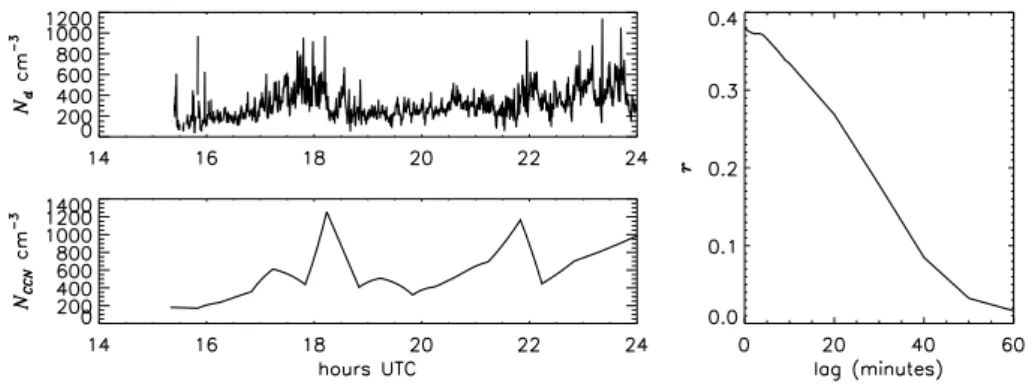
The effect of separation between individual observations of retrieved aerosol and cloud properties on a fine scale can be easily visualized with high temporal resolution ground-based remote sensing data taken from the ARM Mobile Fa-cility, Pt. Reyes deployment. The data in Fig. 8 is represen-tative of the same cloud regime used to initialize the WRF model simulations employed in this study, thus the cloud characteristics are very similar. Ndwas calculated fromτc andL(e.g., Bennartz, 2007) originally sampled at 20 s while NCCN, assumed to vary more slowly, was originally sam-pled at 30 min and then resamsam-pled to match the sampling frequency ofNd. To investigate the effect of separation, we apply increasing lag times between aerosol and cloud data and calculate the cross-correlation. The correlation between NdandNCCNat zero lag time isr=0.38; at a lag time of 5 min (1.5–3 km for an advection velocity of 5–10 ms−1)there is almost no loss in correlation. It is reduced by nearly half (tor=0.18) over a period of 30 min, or over a distance of 10–20 km, and is near zero after a lag time of 60 min.
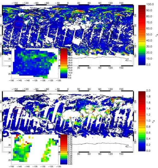
The L2 MODIS scene in Fig. 9 illustrates the separation between aerosol optical depth and cloud optical depth that might influence a global analysis of the albedo effect. In the upper left corner of the scene, thin cloud transitions to thicker cloud toward the lower right. There is no informa-tion on aerosol variability and its potential contribuinforma-tion to cloud variability. It is clear that in this dataset the aerosol properties are not complete with respect to the location of cloud to meet the criteria of a process-scale analysis. While MODIS L2 data provide instantaneous properties with near-global coverage, they are generally not used in near-global-scale analyses due to the enormous volume of data that would be required. In Sect. 5 we propose the use of MODIS L2 data for regional to global analyses of the albedo effect, capitaliz-ing on the variability in aerosol and cloud properties captured in this higher resolution data.
Fig. 6. Statistical parameters variances2, homogeneity parameterγ, and normalized PDFs ofτcfor the native resolution and aggregated
scenes “a”, “b”, and “c” in Fig. 4.
Fig. 7.Statistical parameterrforτcvs.Nafor the native resolution and aggregated scenes from “a”, “b”, and “c” in Fig. 4.
measured simultaneously, aggregation of aerosol and cloud properties over larger areas (time periods) allows for the pop-ulation of geographic locations (times) with measured val-ues, where previously values were missing. This provides co-located properties where they may not have existed at finer resolution. However, this computational aggregation may not preserve statistical accuracy in the variables.
This phenomenon can be observed in the MODIS L3 im-age insets in Fig. 10 that represent the same area of the scenes in Fig. 9 with the same color scales (but different map pro-jections). Note that L3 statistics may not be a function of straightforward averaging of L2 data in space for various reasons. Daily averaged values may result from more than one overpass depending on geographical location (latitude) (Hubanks et al., 2008) and, for 8-day or monthly L3 prod-ucts, sampling issues caused by the satellite orbital
geom-etry, limitations of the retrieval algorithm, and consequent weighting strategies may have a non-negligible impact (Levy et al., 2009). Table 2 provides statistics for this scene at the original (L2) and averaged (L3) resolutions. The percent of co-located aerosol and cloud optical depths increase greatly from 0 in the L2 data (by definition) to 99 % in the L3 data (or 47 % including the swath of missing data in the aerosol optical depth product due to sunglint) but the values also change, becoming more homogeneous. With averaging, the range and variance of theτcdata decreases but the range of τaremains constant which, according to Eq. (2), may impact the relationship between aerosol and cloud in a regression analysis.
Fig. 8.Nd,NCCN, and their lagged cross-correlation from the DOE Pt. Reyes ARM Mobile Facility deployment in 2005.
Fig. 9.MODIS Level 2 data over the northeast Pacific Ocean on 20 July 2001: cloud optical depth (top) at 1 km resolution and aerosol optical depth (bottom) at 10 km resolution.
Table 2. Statistics forτc andτa MODIS L2 and L3 data for the
region in Fig. 8 and the box and inset region in Fig. 9.
min max µ s2 #obs colocation
τc L3L2 0.012.80 6120 8.59.0 449 1,444,271478 0 %99 %∗(47 %)∗∗
τa L2L3 0.010.02 0.30.3 0.070.08 0.0010.001 3599227
∗for the area outside the swath of missing data in the aerosol optical depth scene due
to sunglint.
∗∗for the entire scene including the area of missing data due to sunglint.
Fig. 10. MODIS Level 3 global data on 20 July 2001: cloud optical depth (top) and aerosol optical depth (bottom), both at 1◦resolution. The insets represent the same area as the scenes in Fig. 9 over the northeast Pacific Ocean and have the same color scales.
4.2 Ignoring the constraint on cloud liquid water path
Cloud optical depth and reflectance are highly correlated withL (Schwartz et al., 2002; Kim et al., 2003). Various factors including meteorology and cloud drop microphysi-cal properties can result in variability inτc. By constrain-ing changes inτcbyL, the remaining variability will be due primarily to changes in microphysical properties associated with variation in aerosol. Without this constraint, larger-scale meteorological processes that produce variability in L and thereforeτc will confound detection of aerosol-cloud inter-actions associated with the albedo effect.
When calculating ACI, the constraint onLis often ignored in satellite-based analyses due the difficulty in achieving an independent measure ofLcoincident with other cloud and aerosol properties. When unconstrained, the regression slope is often flattened due to the spread of uncorrelated aerosol and cloud parameters across different L values that exist in varied meteorological conditions. This was shown using ground-based observations from Pt. Reyes (McComiskey et
al., 2009). Here, the PDF sampling methodology described in Sect. 3.4 and outlined in Fig. 5 is applied to WRF model output to illustrate the impact of ignoring the constraint on Lwhen quantifying ACI and to show the robustness of this result.
Fig. 11.Pairs ofNaandτcproduced by a parcel model following
the PDF sampling method in Fig. 5 using aerosol and cloud property inputs derived from the high resolution case of WRF scene “b” in Fig. 4. Grey symbols represent all data points from the modeled scene and colored symbols represent selected 10 g m−2Lbins. The black line represents the unconstrained slope or ACI resulting from all data points and the colored lines represent the slopes for thatL
bin, or selected constrained ACI values.
Plane parallel radiative transfer calculations following Mc-Comiskey and Feingold (2008) shown in Fig. 2 indicate that the difference in constrained versus unconstrained ACI would result in a difference in local (100 % cloud cover) ra-diative forcing of the cloud albedo effect of approximately 3 W m−2 (given a change in CCN from 100 to 300 cm−3, L=125 g m−2) or approximately 0.75 W m−2 for a globe with a 25 % liquid water cloud fraction, discounting 3-D ra-diative transfer effects. This is a potentially important source of bias in observationally based radiative forcing estimates of the albedo effect.
With progressive aggregation of data, the result above holds until the statistical properties of the cloud and aerosol data become too smooth to allow for a valid ACI calculation. Figure 12 shows the constrained and unconstrained ACI val-ues at each level of aggregation for the three scenes in Fig. 4 (top row). A distinct feature is that the difference between constrained and unconstrained ACI values increases as the heterogeneity within the cloud field increases (Fig. 4, top row) from the relatively homogeneous case of closed cells in scene “a” to the open cell, heterogeneous scene “c”. This is clearly an effect of the increasingly disparate values ofL within each scene. The small difference between constrained and unconstrained ACI values in scene “a” for the highest level of aggregation is consistent with the high homogeneity parameter for this case (Fig. 6).
The amount of bias that cloud field heterogeneity produces in quantifying the albedo effect is based on the analysis scale
and heterogeneity of the measured property internal to that unit of observation. In a homogeneous scene, aggregation of properties results in a relatively accurate representation of the finer-scale properties and processes. However, as or-ganization and pattern become more distinct and complex, aggregation will cause loss of information associated with that pattern. At increasingly larger scales, global studies us-ing satellite-based observations lump together various cloud types with widely varying patterns, as well as aerosol with varying properties (Grandey and Stier, 2010). In such cases, the trend of increasing differences between ACI constrained and unconstrained byLwith scene heterogeneity could result in unconstrained ACI values that are biased very low, such as the analyses that fall to the right of the plot in Fig. 1b with resolutions on the order of 4◦.
Figure 12 shows that the unconstrained values of ACI are less than the constrained values in all but a couple of cases. With increasing aggregation, the values of ACI generally fol-low the trends of the statistics presented in Fig. 6, mani-festing some effects of the characteristic length scales of the cloud properties. Distinct increases occur at the highest level of aggregation. In this example, larger ACI values are typi-cally a function of narrow distributions that result from ag-gregation, similar to the narrowing of theτcPDFs in Fig. 6. Similar results were found for the ground-based data from Pt. Reyes in which the days that had naturally low variability in aerosol concentrations did not provide useful ACI values because distributions were too narrow to achieve a meaning-ful regression slope (McComiskey et al., 2009). Here we see that the same result can occur from artificially narrow-ing distributions through aggregation. Generally, this affects data sets in which sample numbers are limited, a problem not encountered in global analyses.
Looking into the individual realizations that make up the ACI values in Fig. 12 provides valuable information for un-derstanding the issues associated with calculating ACI with less-than-ideal data sets. Figure 13 contains the individ-ual ACI calculations (based on Sect. 3.4) from the scene in Fig. 4c, top row for the constrained and unconstrained values at the finest (0.3 km) and coarsest (6 km) resolutions. The set of realizations is stable for both the constrained and un-constrained calculations at 0.3 km resolution and fall within the physically meaningful limits of the relationship (Eq. 1a) between 0 and 0.33. With substantial aggregation to 6 km, spurious values of ACI appear for both constrained and un-constrained calculations, but more so for the unun-constrained calculations. This is due to the fact that aggregation results in fewer data points from which to calculate a regression slope, resulting in an ACI value that is not robust.
Fig. 12.Unconstrained and constrained ACI with change in level of aggregation for scenes “a”, “b”, and “c” in Fig. 4 (top row).
Fig. 13. Constrained (C) and unconstrained (U) ACI for the finest and coarsest resolutions of scene “c” from Fig. 4. Each set of con-strained and unconcon-strained values consists of 30 data points. The horizontal lines at ACI = 0 and 0.33 mark the physical limits of the relationship.
without constraint onLare ipso facto more representative of the full system of aerosol-cloud processes in rapid adjust-ment rather than just the albedo effect. Hence, the range of radiative forcing from observational estimates shown in Fig. 1a (at right), excluding those constrained observations made at the process scale, may also be more representative of the multitude of aerosol-cloud interactions with feedbacks rather than solely the albedo effect. Considering ACI esti-mates from satellite only at a scale of 1◦and larger, that range in forcing, under the same conditions of the calculations in Sect. 2 (factor of 3 increase inNCCN and a global average liquid water cloud cover of 25 % with meanL=125 g m−2) becomes−0.2 to−1.5 W m−2.
5 Observationally-based measurement of ACI using regime-dependent PDFs
We have shown that for processes such as the albedo effect that operate on the microphysical scale, the use of aggregated data results in errors of statistics and sampling, leading to biases in associated radiative forcing estimates. Addition-ally, lack of constraints on the analysis, common with the use of aggregated data, often results in a low bias. How-ever, disaggregated data does not easily lend itself to global coverage and, for regional-to-global scale studies that can address climate issues, data must be scaled-up in a manner that preserves the inherent processes. An approach to an observationally-based estimate of the albedo effect that uses data in conjunction with a process model was outlined pre-viously (Sect. 3.4; Fig. 5) and applied to WRF model output in Figs. 11, 12, and 13. It is detailed here in the context of employing observational data rather than the WRF model output. The objective is to devise an observationally-based approach to radiative forcing estimates and to reduce climate model uncertainty or biases in those estimates. This pro-posed approach preserves the internal heterogeneity of units of observation through the use of PDFs rather than means.
to include sub-adiabaticity using either continuous (e.g., Lee and Pruppacher, 1977) or discrete (Krueger et al., 1997) mix-ing models.
Note that satellite sensors yield independent measure-ments ofreandτc, from whichL(∝re×τc)is derived. The procedure described above is based on a sampling of the PDF of L, but the model generates an internally consistent τc. An important final stage of this procedure is to ensure that the model-generated frequency distribution ofτc conforms, within measurement uncertainties, to the observedτc distri-bution. Lack of agreement would indicate that the model is not capturing the key cloud processes.
Because of the inherent coupling betweenL andw, the fidelity of the calculations can be increased if the depen-dence on the joint distributions of L; w is included, as in Sect. 3. This is especially true under high aerosol loadings wherew plays an increasingly important role in influenc-ing the strength of the cloud response to aerosol (Feinfluenc-ingold, 2003; McComiskey et al., 2009). Recent efforts combining Doppler radar and microwave radiometer are beginning to produce such PDFs (P. Kollias and E. Luke, personal com-munication, 2011) but the extent to which these are depen-dent on cloud regime must be ascertained before they can be applied more generally.
The random sampling of the aerosol and jointL;w distri-butions described above represents the full range of possible couplings between aerosol, cloud water, and updraft veloc-ity characteristics over a given domain. This provides “co-located” sets of aerosol, cloud optical depth, and cloud liq-uid water that span the entire range of likely values in a given regime or geographical location. Sampling these full distri-butions to calculate ACI would provide results with bounds on the potential strength of the albedo effect (the uncertainty in ACI). Typical distributions for different cloud regimes in different geographical locations will result in characteristic globally and temporally distributed ACI values.
An example of data that could be used with this method-ology are PDFs collected over space and time at relatively high spatial resolution, e.g., MODIS L2 data at 1–10 km as presented in Fig. 9. These provide a representative distribu-tion of the properties that occur at a given locadistribu-tion and/or season over the long-term (albeit without vertical velocity) and are, thus, statistically well-constrained. While MODIS L3 data have collated such distributions, the bin designa-tions for some properties are not optimal for this applica-tion, especially those for aerosol. Both ground- and space-based observations including active and passive remote sens-ing can contribute to buildsens-ing such distributions and can pro-vide added dimensionality to the data (e.g., precipitating vs. non-precipitating conditions; Lebsock et al., 2008).
The attractiveness of this method is that it is applicable to observational and model-generated properties and can po-tentially be used in observationally-based radiative forcing estimates as described above, as well as model evaluation and possibly empirical model parameterization. For the
lat-ter, distributions of aerosol, cloud, and updraft velocity pa-rameters within a model grid cell can be used to designate an appropriate value of ACI. Computationally, this would provide a less expensive method than activation parameter-ization schemes but a more accurate approach than global single-value ACI-based estimates. Alternatively, the char-acteristic globally- and seasonally-determined ACI values from the previously described observationally-based analy-sis could be used in models in place of a single, global value.
6 Discussion and conclusions
The influence of aerosol on cloud albedo is recognized as a major unknown. It likely results in planetary cooling, the magnitude of which is poorly constrained. Our contention is that model estimates of the radiative impacts of the albedo effect that are based on observed aerosol-cloud interaction (ACI) metrics are biased due to a mismatch between pro-cess and analysis scales. The historic use of a single measure (ACI) based on data from a range of different observational scales and platforms results in widely varying radiative forc-ing estimates.
Simple numerical aggregation of data to reach a desired geographical scale does not produce the intended, physically meaningful result at that scale. This is readily seen in the lit-erature that addresses the quantification of the microphysical aspect of the albedo effect, as measured here by ACI. The questions raised here extend beyond the albedo effect; the same issues pertain to other metrics of aerosol-cloud interac-tions such as aerosol-cloud fraction relainterac-tionships and aerosol impacts on precipitation such as precipitation susceptibility (e.g., Sorooshian et al., 2009). There the problems are even more difficult because, unlike ACI, they are not constrained by simple physical principles (Eq. 1).
liquid water do not accurately represent the microphysical-scale interactions between aerosol and cloud albedo. This results in biases in radiative forcing estimates of the cloud-albedo effect in GCMs.
The examination of Grandey and Stier (2010) into the im-pacts of scale on quantifying the albedo effect concluded that successive sampling of satellite data from regions of 1◦×1◦ to 60◦×60◦resulted in an associated radiative forcing that
increasedwith coarser resolution. This is in contrast to the ACI results we show in Fig. 1b from studies throughout the literature that span a range of scales. They used a derivation ofNd=f (τcandre)from MODIS that should in principle be independent ofLand thus their results were not affected by lack of constraint onL, but predominately by other aggre-gation effects as discussed in Sect. 2. Here, we have focused on the biases that are incurred in calculation of ACI using aggregated data, which includes all satellite-based observa-tions, as opposed to disaggregated data, which better repre-sents the local microphysical processes. We find that, in this case, simple aggregation biases are dominated by the effect of separation of aerosol and cloud properties in space and time and the lack of constraint onL, resulting in associated radiative forcings that decrease with decreasing resolution. From these two studies it becomes clear that consideration of the scale and approach to quantifying aerosol-cloud inter-actions is essential, with no simple recipe for doing so.
Alternative approaches to quantifying the albedo effect ex-ist and should be capitalized upon. Alternatives may include the combination of multiple available passive and active space-based sensors with airborne and ground-based mea-surements, process-scale modeling, and extrapolation of re-sults using disaggregated data to larger-scales. As the errors in these quantifications are related to cloud field morphol-ogy, considering these approaches on a regime-dependent basis may help to minimize that error. The use of regime-dependent PDFs of aerosol and cloud properties may also lead to progress in observationally-based estimates of the albedo effect as well as datasets that could be used for model evaluation and parameterization. Because it is not currently practical to obtain co-located measures of aerosol and cloud globally, a viable option is to link the needed observations with cloud process models. We have presented a methodol-ogy for such a model-based, observationally-constrained as-sessment of the albedo effect based on sampling of the full range of the PDF of aerosol and the PDF of liquid water path (preferably joint with updraft velocity). The result will be a quantity describing aerosol-cloud interactions that are dic-tated by model physics (determined by cloud regime) and constrained by observations.
What is the appropriate scale at which to observe and char-acterize processes related to aerosol-cloud interactions? It is our assertion that to quantify the albedo effect accurately, disaggregated data (in situ measurements) should be used, or data aggregated only up to the scale that heterogeneity in aerosol and cloud properties is preserved within reasonable
error bounds (e.g., as provided by ground-based remote sens-ing). Accurate measures from aggregated data are possible to the extent that they meet these spatial or temporal hetero-geneity constraints. A brief survey of scales of variability (Sect. 2.2) indicates that 1 km may be a reasonable resolu-tion. If these critical scales are not taken into consideration, a heterogeneity- (and therefore geographical- or regime-) de-pendent bias in ACI will result. Although prior studies have addressed the properties of aerosol and cloud spatial vari-ability, for indirect effects there is the added complexity of assessing the change in covariance properties with the scale of the aerosol and cloud observations. Quantifying length scales of heterogeneity in different cloud regimes to reduce aggregational error in analyses of aerosol-cloud interactions is a non-trivial problem that will require a focused research effort.
Another question that this paper raises is: what does ACI represent? At the core, process level, ACI represents the activation process. At larger scales it must, ipso facto, in-clude other cloud microphysical processes whose contribu-tions vary from one cloud regime to another. To the cli-mate modeler working with grid boxes of order 1◦, ACI must therefore also represent the broader spectrum of cloud micro-physical processes. However, since the albedo effect only at-tempts to address instantaneous impacts of aerosol on cloud albedo without the complications of feedbacks to cloud frac-tion orL, it becomes particularly hard to justify continued use of empirical measures of ACI as a means of assessing the albedo effect. Instead, the full range of aerosol effects on cloud microphysics should be addressed using process-scale measures of ACI (e.g., ∼1 km), unconstrained by L, that have been aggregated to the climate model scale. Moreover, if the measures of ACI have been aggregated appropriately, e.g., using the model-based method described in Sect. 5, then they are more likely to embody causality rather than unphys-ical correlation induced by large-scale averaging.
Acknowledgements. This research was supported by the Office of Science (BER), U.S. Department of Energy, Interagency Agree-ment No. DE-SC0002037. We thank Hailong Wang for providing the cloud resolving model fields in Fig. 5.
Edited by: J. Quaas
References
Ackerman, A., Kirkpatrick, M. P., Stevens, D. E., and Toon, O. B.: The impact of humidity above stratiform clouds on indirect aerosol climate forcing, Nature, 432, doi:10.1038/nature03174, 2004.
Albrecht, B.: Aerosols, cloud microphysics, and fractional cloudi-ness, Science, 245, 1227–1230, 1989.
Anderson, T. L., Charlson, R. J., Winker, D. M., Ogren, J. A., and Holmen, K.: Mesoscale variations of tropospheric aerosols, J. Atmos. Sci., 60, 119–136, 2003.
Asmi, A., Wiedensohler, A., Laj, P., Fjaeraa, A.-M., Sellegri, K., Birmili, W., Weingartner, E., Baltensperger, U., Zdimal, V., Zikova, N., Putaud, J.-P., Marinoni, A., Tunved, P., Hansson, H.-C., Fiebig, M., Kivek¨as, N., Lihavainen, H., Asmi, E., Ulevicius, V., Aalto, P. P., Swietlicki, E., Kristensson, A., Mihalopoulos, N., Kalivitis, N., Kalapov, I., Kiss, G., de Leeuw, G., Henzing, B., Harrison, R. M., Beddows, D., O’Dowd, C., Jennings, S. G., Flentje, H., Weinhold, K., Meinhardt, F., Ries, L., and Kulmala, M.: Number size distributions and seasonality of submicron par-ticles in Europe 20082009, Atmos. Chem. Phys., 11, 5505–5538, doi:10.5194/acp-11-5505-2011, 2011.
Barker, H.: A Parameterization for Computing Grid-Averaged Solar Fluxes for Inhomogeneous Marine Boundary Layer Clouds. Part I: Methodology and Homogeneous Biases, J. Atmos. Sci., 53, 2289–2303, 1996.
Bennartz, R.: Global assessment of marine boundary layer cloud droplet number concentration from satellite, J. Geophys. Res., 112, D02201, doi:10.1029/2006JD007547, 2007.
Bony, S. and Dufrense, J.-L.: Marine boundary layer clouds at the heart of tropical feedback uncertainties in climate models, Geo-phys. Res. Lett., 32, L20806, doi:10.1029/2005GL023851, 2005. Brenguier, J.-L.: Observation of cloud microstructure at the
cen-timeter scale, J. Appl. Meteor., 32, 783–793, 1993.
Brenguier, J.-L., Pawlowska, H., and Schuller, L.: Cloud micro-physical and radiative properties for parameterization and satel-lite monitoring of the indirect effect of aerosol on climate, J. Geo-phys. Res., 108, 8632, doi:10.1029/2002JD002682, 2003a. Brenguier, J.-L., Chuang, P. Y., Fouquart, Y., Johnson, D. W.,
Parol, F., Pawlowska, H., Pelon, J., Sch¨uller, L., Schr¨oder, F., and Snider, J.: An overview of the ACE-2 CLOUDYCOLUMN closure experiment, Tellus B, 52, 815–827, doi:10.1034/j.1600-0889.2000.00047.x, 2003b.
Br´eon, F.-M., Tanre, D., and Generoso, S.: Aerosol Effect on Cloud Droplet Size Monitored from Satellite, Science, 295, 834, doi:10.1126/science.1066434, 2002.
Bulgin, C. E., Palmer, P. I., Thomas, G. E., Arnold, C. P. G., Campmany, E., Carboni, E., Grainger, R. G., Poulsen, C., Siddans, R., and Lawrence, B. N.: Regional and seasonal variations of the Twomey indirect effect as observed by the ATSR-2 satellite instrument, Geophys. Res. Lett., 35, L02811, doi:10.1029/2007GL031394, 2008.
Chameides, W. L., Luo, C., Saylor, R., Streets, D., Huang, Y., Bergin, M., and Giorgi, F: Correlations between model-calculated anthropogenic aerosols and satellite-derived cloud op-tical depths: Indication of indirect effect?, J. Geophys. Res, 107, 4085, doi:10.1029/2000JD000208, 2002.
Davis, A., Marshak, A., Cahalan, R., and Wiscombe, W.: The Land-sat scale break in stratocumulus as a three-dimensional radiative transfer effect: Implications for cloud remote sensing, J. Atmos. Sci., 54, 241–260, 1997.
Feingold, G.: Modeling of the first indirect effect: Analysis of measurement requirements, Geophys. Res. Lett., 30, 1997, doi:10.1029/2003gl017967, 2003.
Feingold, G. and Heymsfeld, A.: Parameterizations of the conden-sational growth of droplets for use in GCMs, J. Atmos. Sci. 49, 2325–2342, 1992.
Feingold, G., Remer, L. A., Ramaprasad, J., and Kaufman, Y. J.: Analysis of smoke impact on clouds in Brazilian biomass burn-ing regions: An extension of Twomey’s approach, J. Geophys. Res., 106, 22907–22922, 2001.
Feingold, G., Eberhard, W. L., Veron, D. E., and Previdi, M.: First measurements of the Twomey indirect effect using ground-based remote sensors, Geophys. Res. Lett., 30, 1287, doi:10.1029/2002GL016633, 2003.
Forster, P., Ramaswamy, V., Artaxo, P., Berntsen, T., Betts, R., Fa-hey, D. W., Haywood, J., Lean, J., Lowe, D. C., Myhre, G., Nganga, J., Prinn, R., Raga, G., Schulz, M., and Van Dorland, R.: Changes in atmospheric constituents and in radiative forcing, in Climate Change 2007: The Physical Science Basis – Con-tribution of Working Group I to the Fourth Assessment Report of the Intergovernmental Panel on Climate Change, edited by: Solomon, S., Qin, D., Manning, M., Chen, Z., Marquis, M., Av-eryt, K. B., Tignor, M., and Miller, H. L., 289–348, Cambridge Univ. Press, New York, 2007.
Fotheringham, A. S. and Wong, D. W.: The modifiable areal unit problem in multivariate statistical analysis, Environment and Planning A, 23, 1025–1044, 1991.
Garrett, T. J., Zhao, C., Dong, X., Mace, G. G., and Hobbs, P. V.: Effects of varying aerosol regimes on low-level Arctic stratus, Geophys. Res. Lett., 31, L17105, doi:10.1029/2004GL019928, 2004.
Gerber, H., Jensen, J. B., Davis, A. B., Marshak, A., and Wiscombe, W. J.: Spectral density of cloud liquid water content at high fre-quencies, J. Atmos. Sci., 58, 497–503, 2001.
Grandey, B. S. and Stier, P.: A critical look at spatial scale choices in satellite-based aerosol indirect effect studies, Atmos. Chem. Phys., 10, 11459–11470, doi:10.5194/acp-10-11459-2010, 2010. Gultepe, I., Isaac, G. A., Leaitch, W. R., and Banic, C. M.: Param-eterizations of marine stratus microphysics based on in-situ ob-servations: Implications for GCMs, J. Clim., 9, 345–357, 1996. Hubanks, P. A., King, M. D., Platnick, S., and Pincus, R.: MODIS
Atmosphere L3 Gridded Product Algorithm Theoretical Basis Document, MODIS Algorithm Teoretical Basis Document No. ATBD-MOD-30, 2008.
Jelinski, D. E. and Wu, J.: The modifiable areal unit problem and implications for landscape ecology, Landscape Ecology, 11, 129–140, 1996.
Kaufman, Y. J., Koren, I., Remer, L. A., Rosenfeld, D., and Rudich, Y.: The effect of smoke, dust, and pollution aerosol on shallow cloud development over the Atlantic Ocean, P. Natl. Acad. Sci., 102, 11207–11212, doi:10.1073/pnas.0505191102, 2005. Kim, B.-G., Schwartz, S. E., Miller, M. A., and Min, Q.:
Ef-fective radius of cloud droplets by ground-based remote sens-ing: Relationship to aerosol, J. Geophys. Res., 108, 4740, doi:10.1029/2003JD003721, 2003.
Kim, B.-G., Miller, M. A., Schwartz, S. E., Liu, Y., and Min, Q.: The role of adiabaticity in the aerosol first indirect effect, J. Geo-phys. Res., 113, D05210, doi:10.1029/2007JD008961, 2008. Krueger, S. K., Su, C.-W., and McMurtry, P. A.: Modeling
Entrain-ment and Finescale Mixing in Cumulus Clouds, J. Atmos. Sci., 54, 2697–2712, 1997.
growth of cloud droplets by condensation using an air parcel morel with and without entrainment, Pure Appl. Geophys., 115, 523–545, 1977.
Lebsock M. D., Stephens, G. L., and Kummerow, C.: Multisensor satellite observations of aerosol effects on warm clouds, J. Geo-phys. Res., 113, D15205, doi:10.1029/2008JD009876, 2008. Lee, I.-Y. and Pruppacher, H. R.: A comparative study on the
growth of cloud drops by condensation using an air parcel model with and without entrainment, Pure Appl. Geophys., 115, 523– 545, doi:10.1007/BF00876119, 1977.
Levy, R. C., Leptoukh, G. G., Kahn, R., Zubko, V., Gopalan, A., and Remer, L. A.: A Critical Look at Deriving Monthly Aerosol Op-tical Depth From Satellite Data, IEEE T. Geosci. Remote Sens., 47, 2942–2956, doi:10.1109/TGRS.2009.2013842, 2009. Lihavainen, H., Kerminen, V.-M., Komppula, M., Hyv¨arinen, A.-P.,
Laakia, J., Saarikoski, S., Makkonen, U., Kivek¨as, N., Hillamo, R., Kulmala, M., and Viisanen, Y.: Measurements of the relation between aerosol properties and microphysics and chemistry of low level liquid water clouds in Northern Finland, Atmos. Chem. Phys., 8, 6925–6938, doi:10.5194/acp-8-6925-2008, 2008. Lohmann, U., Rotstayn, L., Storelvmo, T., Jones, A., Menon, S.,
Quaas, J., Ekman, A. M. L., Koch, D., and Ruedy, R.: Total aerosol effect: radiative forcing or radiative flux perturbation?, Atmos. Chem. Phys., 10, 3235–3246, doi:10.5194/acp-10-3235-2010, 2010.
Lu, M.-L., Conant, W. C., Jonsson, H. H., Varutbangkul, V., Fla-gan, R. C., and Seinfeld, J. H.: The Marine Stratus/ Stra-tocumulus Experiment (MASE): Aerosol-cloud relationships in marine stratocumulus, J. Geophys. Res., 112, D10209, doi:10.1029/2006JD007985, 2007.
Lu, M.-L., Feingold, G., Jonsson, H. H., Chuang, P. Y., Gates, H., Flagan, R. C., and Seinfeld, J. H.: Aerosol-cloud relationships in continental shallow cumulus, J. Geophys. Res., 113, D15201, doi:10.1029/2007JD009354, 2008.
Martin, G. M., Johnson, D. W., and Spice, A.: The measurement and parameterization of effective radius of droplets in warm stra-tocumulus clouds, J. Atmos. Sci., 51, 1823–1842, 1994. Matsui, T., Masunaga, H., Kreidenweis, S. M., Pielke, R. A., Tao,
W.-K., Chin, M., and Kaufman, Y. J.: Satellite-based assessment of marine low cloud variability associated with aerosol, atmo-spheric stability, and the diurnal cycle, J. Geophys. Res., 111, D17204, doi:10.1029/2005JD006097, 2006.
McComiskey, A. and Feingold, G.: Quantifying error in the ra-diative forcing of the first aerosol indirect effect, Geophys. Res. Lett., 35, L02810, doi:10.1029/2007GL032667, 2008.
McComiskey, A., Feingold, G., Frisch, A. S., Turner, D. D., Miller, M. A., Chiu, J. C., Min, Q., and Ogren, J. A.: An assess-ment of aerosol-cloud interactions in marine stratus clouds based on surface remote sensing, J. Geophys. Res., 114, D09203, doi:10.1029/2008JD011006, 2009.
McFarquhar, G. M. and Heymsfield, A. J.: Parameterizations of INDOEX microphysical measurements and calculations of cloud susceptibility: Applications for climate studies, J. Geophys. Res., 106, 28675–28698, 2001.
Medeiros, B., Stevens, B., Held, I. M., Zhao, M., Williamson, D. L., Olson, J. G., and Bretherton, C. S.: Aquaplanets, Climate Sensitivity, and Low Clouds, J. Clim., 21, 4974–4991, 2008. Murphy, D., Solomon, S., Portmann, R., Rosenlof, K., Forster,
P., and Wong, T.: An observationally based energy balance
for the Earth since 1950, J. Geophys. Res., 114, D17107, doi:10.1029/2009jd012105, 2009.
Nakajima, T., Higurashi, A., Kawamoto, K., and Penner, J. E.: A possible correlation between satellite-derived cloud and aerosol micro- physical parameters, Geophys. Res. Lett., 28, 1171–1174, 2001.
O’Dowd, C. D., Lowe, J. A., Smith, M. H., and Kaye, A. D.: The relative importance of sea-salt and nss- sulphate aerosol to the marine CCN population: An improved multi- component aerosol-droplet parameterization, Q. J. Roy. Meteorol. Soc., 125, 1295–1313, 1999.
Openshaw, S.: The Modifiable Areal Unit Problem, Concepts and Techniques in Modern Geography, No. 38, 1984.
Oreopolous, L., Marshak, A., Cahalan, R. F., and Wen, G.: Cloud three-dimensional effects evidenced in Landsat spatial power spectra and autocorrelation functions, J. Geophys. Res., 105, 14777–14788, 2000.
Platnick, S., King, M. D., Ackerman, S. A., Menzel, W. P., Baum, B. A., Ri´edi, J. C., and Frey, R. A.: The MODIS Cloud Products: Algorithms and Examples From Terra, IEEE T. Geosci. Remote, 41, 459–473, 2003.
Quaas, J., Boucher, O., and Breon, F.-M.: Aerosol indirect effects in POLDER satellite data and the Laboratoire de Meteorologie Dynamique–Zoom (LMDZ) general circulation model, J. Geo-phys. Res., 109, D08205, doi:10.1029/2003JD004317, 2004. Quaas, J., Boucher, O., and Lohmann, U.: Constraining the
to-tal aerosol indirect effect in the LMDZ and ECHAM4 GCMs using MODIS satellite data, Atmos. Chem. Phys., 6, 947–955, doi:10.5194/acp-6-947-2006, 2006.
Quaas, J., Boucher, O., Bellouin, N., and Kinne, S.: Satellite-based estimate of the direct and indirect aerosol climate forcing, J. Geo-phys. Res., 113, D05204, doi:10.1029/2007JD008962, 2008. Quaas, J., Ming, Y., Menon, S., Takemura, T., Wang, M., Penner,
J. E., Gettelman, A., Lohmann, U., Bellouin, N., Boucher, O., Sayer, A. M., Thomas, G. E., McComiskey, A., Feingold, G., Hoose, C., Kristj´ansson, J. E., Liu, X., Balkanski, Y., Donner, L. J., Ginoux, P. A., Stier, P., Grandey, B., Feichter, J., Sednev, I., Bauer, S. E., Koch, D., Grainger, R. G., Kirkev˚ag, A., Iversen, T., Seland, Ø., Easter, R., Ghan, S. J., Rasch, P. J., Morrison, H., Lamarque, J.-F., Iacono, M. J., Kinne, S., and Schulz, M.: Aerosol indirect effects general circulation model intercompar-ison and evaluation with satellite data, Atmos. Chem. Phys., 9, 8697–8717, doi:10.5194/acp-9-8697-2009, 2009.
Raga, G. B. and Jonas, P. R.: On the link between cloud-top radia-tive properties and sub-cloud aerosol concentrations, Q. J. Roy. Meteorol. Soc., 119, 1419–1425, 1993.
Ramanathan, V., Crutzen, J., Kiehl, J. T., and Rosenfeld, D.: Aerosols, climate, and the hydrological cycle, Science, 294, 2119–2124, 2001.
Remer, L. A., Kaufman, Y. J., Tanre, D., Matoo, S., Chu, D. A., Martins, J. V., Li, R.-R., Ichoku, C., Levy, R. C., Kleidman, R. G., Eck, T. F., Vermote, E., and Holben, B. N.: The MODIS Aerosol Algorithm, Products, and Validation, J. Atmos. Sci., 62, 947–973, 2005.
Robinson, W. S.: Ecological Correlations and the Behavior of Indi-viduals, American Sociological Review, 15, 351–357, 1950. Schwartz, S. E., Harshvardhan, and Benkovitz, C. M.: Influence of
anthropogenic aerosol on cloud optical depth and albedo shown by satellite measurements and chemical transport modeling, P. Natl. Acad. Sci., 99, 1784–1789, 2002.
Sekiguchi, M., Nakajima, T., Suzuki, K., Kawamoto, K., Higurashi, A., Rosenfeld, D., Sano, I., and Mukai, S.: A study of the direct and indirect effects of aerosols using global satellite data sets of aerosol and cloud parameters, J. Geophys. Res., 108, 4699, doi:10.1029/2002JD003359, 2003.
Shinozuka, Y. and Redemann, J.: Horizontal variability of aerosol optical depth observed during the ARCTAS airborne experiment, Atmos. Chem. Phys., 11, 8489–8495, doi:10.5194/acp-11-8489-2011, 2011.
Sorooshian, A., Feingold, G., Lebsock, M. D., Jiang, H. L., and Stephens, G. L.: On the precipitation susceptibility of clouds to aerosol perturbations. Geophys. Res. Lett., 36, L13803, doi:10.1029/2009GL038993, 2009.
Stevens, B., Lenschow, D. H., Vali, G., Gerber, H., Bandy, A., Blomquist, B., Brenguier, J.-L., Bretherton, C. S., Burnet, F., Campos, T., Chai, S., Faloona, I., Friesen, D., Haimov, S., Laursen, K., Lilly, D. K., Loehrer, S. M., Malinowski, S. P., Morley, B., Petters, M. D., Rogers, D. C., Russell, L., Savic-Jovcic, V., Snider, J. R., Straub, D., Szumowski, M. J., Takagi, H., Thornton, D. C., Tschudi, M., Twohy, C., Wetzel, M., and van Zanten, M. C.: Dynamics and Chemistry of Marine Stra-tocumulus – DYCOMS-II, B. Am. Meteorol. Soc., 84, 579–593, doi:10.1175/BAMS-84-5-579, 2003.
Twomey, S.: Pollution and the planetary albedo, Atmos. Environ., 8, 1251–1256, 1974.
Twohy, C. H., Petters, M. D., Snider, J. R., Stevens, B., Tahnk, W., Wetzel, M., Russell, L., and Burnet, F.: Evaluation of the aerosol indirect effect in marine stratocumulus clouds: Droplet number, size, liquid water path, and radiative impact, J. Geophys. Res., 110, D08203, doi:10.1029/2004JD005116, 2005.
Wang, H. and Feingold, G.: Modeling Mesoscale Cellular Struc-tures and Drizzle in Marine Stratocumulus. Part I: Impact of Drizzle on the Formation and Evolution of Open Cells, J, Atmos. Sci., 66, 3237–3256, doi:10.1175/2009JAS3022.1, 2009. Wood, R. and Hartmann, D. L.: Spatial Variability of Liquid Water
Path in Marine Low Cloud: The Importance of Mesoscale Cellu-lar Convection, J. Clim., 19, 1748–1764, 2006.
Xue, H., Feingold, G., and Stevens, B.: Aerosol effects on clouds, precipitation, and the organization of shallow cumulus convec-tion, J. Atmos. Sci., 65, 392–406; doi:10.1175/2007JAS2428.1, 2008.