Wave-equation based traveltime seismic tomography – Part 1: Method

(1)

SED

6, 2523–2566, 2014

Wave-equation seismic tomography

– Part 1: Method

P. Tong et al.

Title Page

Abstract Introduction

Conclusions References

Tables Figures

◭ ◮

Back Close

Full Screen / Esc

Printer-friendly Version Interactive Discussion

Discussion

P

a

per

|

Discus

sion

P

a

per

|

Discussion

P

a

per

|

Discussion

P

a

per

|

Solid Earth Discuss., 6, 2523–2566, 2014 www.solid-earth-discuss.net/6/2523/2014/ doi:10.5194/sed-6-2523-2014

This discussion paper is/has been under review for the journal Solid Earth (SE). Please refer to the corresponding final paper in SE if available.

Wave-equation based traveltime seismic

tomography – Part 1: Method

P. Tong1, D. Zhao2, D. Yang3, X. Yang4, J. Chen4, and Q. Liu1

1

Department of Physics, University of Toronto, Toronto, M5S 1A7, Ontario, Canada

2

Department of Geophysics, Tohoku University, Sendai, Japan

3

Department of Mathematical Sciences, Tsinghua University, Beijing, China

4

Department of Mathematics, University of California, Santa Barbara, California, USA

Received: 10 August 2014 – Accepted: 11 August 2014 – Published: 25 August 2014

Correspondence to: P. Tong (tongping85@gmail.com)

(2)

SED

6, 2523–2566, 2014

P. Tong et al.

Title Page

Tables Figures

◭ ◮

Back Close

Full Screen / Esc

Discussion

P

a

per

|

Discus

sion

P

a

per

|

Discussion

P

a

per

|

Discussion

P

a

per

|

Abstract

In this paper, we propose a wave-equation based traveltime seismic tomography method with a detailed description of its step-by-step process. First, a linear relation-ship between the traveltime residual ∆t=Tobs−Tsyn and the relative velocity pertur-bation δc(x)/c(x) connected by a finite-frequency traveltime sensitivity kernel K(x) 5

is theoretically derived using the adjoint method. To accurately calculate the traveltime residual∆t, two automatic arrival-time picking techniques including the envelop energy ratio method and the combined ray and cross-correlation method are then developed to compute the arrival timesTsynfor synthetic seismograms. The arrival times Tobs of observed seismograms are usually determined by manual hand picking in real applica-10

tions. Traveltime sensitivity kernelK(x) is constructed by convolving a forward wavefield

u(t,x) with an adjoint wavefieldq(t,x). The calculations of synthetic seismograms and sensitivity kernels rely on forward modelling. To make it computationally feasible for to-mographic problems involving a large number of seismic records, the forward problem is solved in the two-dimensional (2-D) vertical plane passing through the source and 15

the receiver by a high-order central difference method. The final model is parameter-ized on 3-D regular grid (inversion) nodes with variable spacings, while model values on each 2-D forward modelling node are linearly interpolated by the values at its eight surrounding 3-D inversion grid nodes. Finally, the tomographic inverse problem is for-mulated as a regularized optimization problem, which can be iteratively solved by either 20

the LSQR solver or a non-linear conjugate-gradient method. To provide some insights into future 3-D tomographic inversions, Fréchet kernels for different seismic phases are also demonstrated in this study.

1 Introduction

Seismic tomography is one of the core methodologies for imaging the structural hetero-25

(3)

SED

6, 2523–2566, 2014

P. Tong et al.

Title Page

Tables Figures

◭ ◮

Back Close

Full Screen / Esc

Discussion

P

a

per

|

Discus

sion

P

a

per

|

Discussion

P

a

per

|

Discussion

P

a

per

|

Aki and Lee (1976) and Dziewonski et al. (1977), tomographic images have provided crucial information to the understanding of plate tectonics, volcanism and geodynam-ics (e.g. Romanowicz, 1991; Liu and Gu, 2012; Zhao, 2012). Seismic tomography itself also went through significant development over the last three decades, including ad-vances in both methodology and data usage.

5

In the first two decades of its history, seismic tomography is mainly based on the ray theory which assumes that seismic traveltime is determined by the structure along the infinitely thin ray path only. However, because of scattering, wave front healing and other finite-frequency effects, seismic measurements (such as traveltime and amplitude), especially those made on broadband recordings, are sensitive to three-10

dimensional (3-D) structures offthe ray path (e.g. Marquering et al., 1999; Dahlen et al., 2000; Tape et al., 2007). Ray theory is actually only valid when the scale length of the variation of material properties is much larger than the seismic wavelength (Rawlinson et al., 2010). To take into account the influence of off-ray structures, finite-frequency tomography methods in which 2-D or 3-D traveltime and amplitude sensitivity kernels 15

are constructed, including those based on the paraxial approximation and dynamic ray tracing (e.g. Marquering et al., 1999; Dahlen et al., 2000; Tian et al., 2007; Tong et al., 2011) and those based on the normal mode theory (e.g. Zhao et al., 2000; Zhao and Jordan, 2006; To and Romanowicz, 2009). Tomographic models with improved resolutions were reported by recent finite-frequency tomographic studies (e.g. Montelli 20

et al., 2004; Hung et al., 2004, 2011; Gautier et al., 2008), although comparison to ray-based tomography remains controversial (de Hoop and van der Hilst, 2005a; Dahlen and Nolet, 2005; de Hoop and van der Hilst, 2005b). The underlying problem of the finite-frequency tomography based on paraxial approximation and dynamic ray tracing is that its kernel computation still relies on the ray theory, although it was devised to ac-25

(4)

SED

6, 2523–2566, 2014

P. Tong et al.

Title Page

Tables Figures

◭ ◮

Back Close

Full Screen / Esc

Discussion

P

a

per

|

Discus

sion

P

a

per

|

Discussion

P

a

per

|

Discussion

P

a

per

|

et al., 2007). This opens the way to compute sensitivity kernels based on numerical simulation of the full seismic wavefield, avoiding the use of approximate theories (e.g. Liu and Tromp, 2006, 2008; Fichtner et al., 2009). It also made the conceptual wave-equation based seismic inversion methods such as the one presented by Tarantola (1984) feasible in realistic applications (Tape et al., 2009; Fichtner and Trampert, 2011; 5

Zhu et al., 2012). To our best knowledge, adjoint tomography (Tromp et al., 2005; Ficht-ner et al., 2006), scattering integral methods (L. Zhao et al., 2005; Chen et al., 2007b), and full waveform inversion (FWI) in the frequency domain (Pratt and Shipp, 1999; Operto et al., 2006) are among the most popular tomographic techniques based upon solving full wave equations. FWI in frequency domain has been mainly used in explo-10

ration problems (e.g. Virieux and Operto, 2009; Lee et al., 2010) for relative small and regular simulation domains. Adjoint tomography and scattering integral tomography are closely related to each other, and a detailed comparison between adjoint tomography and scattering integral tomography can be found in Chen et al. (2007a). For brevity, we restrict our following discussions to adjoint tomography (Liu and Gu, 2012).

15

Adjoint tomography is currently one of the most popular and promising tomographic methods for resolving strongly varying structures. It takes advantages of full 3-D nu-merical simulations in forward modelling and sensitivity kernel calculation, often iter-atively improves models through optimization techniques (Tromp et al., 2005; Tape et al., 2007). The use of full numerical simulations allows for the freedom of choosing 20

either 1-D or 3-D reference models and accurate calculations of seismograms (Tong et al., 2014a) and sensitivity kernels for complex models (Liu and Tromp, 2006, 2008). Using this approach, Tape et al. (2009, 2010) obtained a 3-D velocity model of the southern California crust that captures strong local heterogeneity up to ±30 %. Simi-larly, Zhu et al. (2012) generated a tomographic model of the European upper mantle 25

based on adjoint tomography that reveals nice correlations between structural features and regional tectonics and dynamics. Similarly, Rickers et al. (2013) presented a 3-D

(5)

SED

6, 2523–2566, 2014

P. Tong et al.

Title Page

Tables Figures

◭ ◮

Back Close

Full Screen / Esc

Discussion

P

a

per

|

Discus

sion

P

a

per

|

Discussion

P

a

per

|

Discussion

P

a

per

|

the promising future of next generation seismic tomographic models based on full nu-merical simulations. However, the expensive computation cost associated with adjoint-type of wave-equation-based tomographic methods, especially for 3-D problems, is still a major stumbling block to its wider applications. For example, for a moderate number of three-component seismograms, 0.8 million and 2.3 million central processing unit 5

hours were used to generate the tomographic models of the southern California crust and the European upper mantle, respectively (Tape et al., 2009; Zhu et al., 2012). The severity of the cost issue may be remedied when simulations are ported to the Graphic Processing Unit (GPU) hardwares (e.g. Komatitsch et al., 2010; Michéa and Komatitsch, 2010). However, ray-based tomographic methods remains the most popu-10

lar and accessible techniques in mapping the heterogeneous structures of the Earth’s interior (e.g. Li et al., 2008; Hung et al., 2011; Tong et al., 2012; Zhao et al., 2012).

As mentioned above, full 3-D numerical simulations in forward modelling and sitivity kernel calculations guarantee the accuracy of synthetic seismograms and sen-sitivity kernels for 3-D complex models. But they also make adjoint tomography com-15

putationally demanding and even unaffordable. To strike a balance between the com-putational efficiency and accuracy of full wave-equation based tomographic methods, we propose to conduct the forward modelling and sensitivity kernel calculation in the 2-D source-receiver vertical plane by a high-order finite-difference scheme. As we will show, if only traveltime measurements are considered, this 2-D approximation offers 20

acceptable accuracy. Meanwhile, by numerically solving 2-D wave equations, finite-frequency effects such as wavefront healing are naturally taken into account, and the accuracy of sensitivity kernels in complex heterogeneous models is also improved. Al-though forward modellings are restricted to 2-D planes, we still plan to invert for 3-D tomographic models on a 3-D inversion grid. The 2-D forwarding modelling and the 3-D 25

(6)

SED

6, 2523–2566, 2014

P. Tong et al.

Title Page

Tables Figures

◭ ◮

Back Close

Full Screen / Esc

Discussion

P

a

per

|

Discus

sion

P

a

per

|

Discussion

P

a

per

|

Discussion

P

a

per

|

(WETST). Comparing with the 3-D-3-D adjoint tomography based on the spectral el-ement method (Tromp et al., 2005; Fichtner et al., 2006), this 2-D-3-D WETST based upon a 2-D finite-difference scheme is generally more computationally affordable. This also entails that WETST can be applied to tomographic inversions involving significant amount of data based on even moderate computational resources.

5

Arrival time picking is another important issue for traveltime seismic tomography. Since the early era of ray-based seismic tomography, researchers have mainly relied on manually picked arrival times to map subsurface structures (e.g. Aki and Lee, 1976; Zhao et al., 1992). Arrival times are usually picked within time windows centred at the predicted traveltimes (Kennett and Engdah, 1991; Maggi et al., 2009). In recent years, 10

increasingly number of deployed broadband seismic arrays have resulted in the prolif-eration of seismic data. To increase efficiency and reduce the amount of manual labour and human errors in seismic data processing, fast and automatic traveltime picking algorithms with high accuracy are highly demanded to process vast amount of seis-mic recordings. Indeed, various techniques have been presented for automatic/semi-15

automatic detecting and picking the arrivals of different seismic phases, and the most widely used of which is the short-term-average (STA) to long-term-average (LTA) ratio method and its variations (e.g. Coppens, 1985; Baer and Kradolfer, 1987; Saari, 1991; Earle and Shearer, 1994; Han et al., 2010). Zhang et al. (2003) developed an auto-maticP wave arrival detection and picking algorithm based on the wavelet transform 20

and Akaike information criteria. Cross-correlation method is another routinely used technique to obtain the traveltime anomalies of broadband pulses, which is specially favoured by finite-frequency tomographic applications (e.g. Luo and Schuster, 1991; Dahlen et al., 2000; Tape et al., 2007). However, the quality of picked arrivals by these methods may vary in accuracy for datasets of different signal-to-noise ratio (SNR), and 25

(7)

pro-SED

6, 2523–2566, 2014

P. Tong et al.

Title Page

Tables Figures

◭ ◮

Back Close

Full Screen / Esc

Discussion

P

a

per

|

Discus

sion

P

a

per

|

Discussion

P

a

per

|

Discussion

P

a

per

|

pose two different automatic arrival-time determination methods (Sect. 3) that forms an integral part of our wave-equation based traveltime seismic tomography method.

When arrival-time data and sensitivity kernels are determined or computed, wave-equation based traveltime seismic tomography is cast as an optimization problem. Model parameterization, regularization and methods solving the optimization problem 5

are discussed in Sects. 4 and 5. Finally, examples of sensitivity kernels for different seismic waves are shown in Sect. 6, which provide the basis for future tomographic inversions with various seismic phases. This paper focuses on theoretical derivation of the wave-equation based traveltime seismic tomography. An application of the WETST method is presented in the second paper (Tong et al., 2014b).

10

2 Tomographic equation

In this section, we set up a linear relationship between the perturbation of arrival time and velocity perturbation in a reference model.

2.1 Traveltime residual

Traveltime seismic tomography generally inverts traveltime residuals of some seismic 15

phases to map the internal Earth structures. A traveltime residual∆tcorresponding to the event occurred atx_sand the seismic station located atx_ris written as,

∆t=Tobs₋_Tsyn_, ₍₁₎

where the observed traveltimeTobs is automatically or manually picked on recorded seismogramd(t), and the synthetic arrival timeTsynis predicted based on a reference 20

model. In geometrical ray theory,Tsynis usually computed by integrating the slowness along a travelling path.

(8)

SED

6, 2523–2566, 2014

P. Tong et al.

Title Page

Tables Figures

◭ ◮

Back Close

Full Screen / Esc

Discussion

P

a

per

|

Discus

sion

P

a

per

|

Discussion

P

a

per

|

Discussion

P

a

per

|

(Dahlen et al., 2000)

∆t≈ 1 Nr

T

Z

0

w(t) ˙u(t) [d(t)−u(t)] dt, (2)

where

Nr=

T

Z

0

w(t)u(t) ¨u(t)dt

and w(t) is a weight function over the time interval [0,T] that can be used to isolate 5

particular seismic phases (Tromp et al., 2005). The accuracy of this approximation improves as data and synthetic pulse becomes more similar, i.e., waveform perturba-tion d(t)−u(t) in Eq. (2) becomes tiny. Assuming infinitesimal perturbations, Eq. (2) becomes

δt= 1

Nr

T

Z

0

w(t) ˙u(t)δu(t) dt, (3)

10

which is used further to set up the relationship between traveltime residual and velocity perturbation.

2.2 Relation between traveltime residual and velocity perturbation

We consider seismic wave propagation in a two-dimensional (2-D) vertical plane which contains the source x_s and the receiver x_r. Within this plane, seismic wavefield of 15

(9)

SED

6, 2523–2566, 2014

P. Tong et al.

Title Page

Tables Figures

◭ ◮

Back Close

Full Screen / Esc

Discussion

P

a

per

|

Discus

sion

P

a

per

|

Discussion

P

a

per

|

Discussion

P

a

per

|

acoustic wave equation with initial and boundary conditions,

   

  

∂2

∂t2u(t,x)=∇ · h

c2(x)∇u(t,x)i+f(t)δ(x−x_s), x∈S u(0,x)=∂u(0,x)/∂t=0, x∈S,

ˆ

n·hc2(x)∇u(t,x)i=0, x∈∂S.

(4)

whereu(t,x) is the displacement field,c(x) is the eitherP orS wave velocity model,

f(t) is the source time function for the point source atx_s, andnˆ is the normal direction of the boundary ∂S. For a perturbation δc(x) of the velocity model c(x), a conse-5

quent perturbed displacement wavefield δu(t,x) will be generated. In the framework of first-order or Born approximation (e.g. Aki and Richards, 2002; Tromp et al., 2005; Tong et al., 2011), the perturbed wavefieldδu(t,x) is the solution to the following wave equation with subsidiary conditions,

   

  

∂2

∂t2δu(t,x)=∇ · h

c2(x)∇δu(t,x)+2c(x)δc(x)∇u(t,x)i, x∈S,

δu(0,x)=∂δu(0,x)/∂t=0, x∈S,

ˆ

n·hc2(x)∇δu(t,x)+2c(x)δc(x)∇u(t,x)i=0, x∈∂S.

(5) 10

Multiply an arbitary test functionq(t,x) on both sides of the first equation in Eq. (5) and then integrate in the surfaceS and the time interval [0,T], we have

T

Z

0 dt

Z

S

q(t,x) ∂ 2

∂t2δu(t,x)dx (6)

=

T

Z

0 dt

Z

S

q(t,x)∇ ·hc2(x)∇δu(t,x)+2c(x)δc(x)∇u(t,x)idx

(10)

SED

6, 2523–2566, 2014

P. Tong et al.

Title Page Abstract Introduction Conclusions References Tables Figures ◭ ◮ ◭ ◮ Back Close

Full Screen / Esc

Printer-friendly Version Interactive Discussion Discussion P a per | Discus sion P a per | Discussion P a per | Discussion P a per |

which is equal to

Z S dx T Z 0 ( ∂ ∂t

q(t,x) ∂

∂tδu(t,x)−δu(t,x) ∂ ∂tq(t,x)

+δu(t,x) ∂ 2

∂t2q(t,x)

)

dt (7)

= T Z 0 dt Z S

δu(t,x)∇ ·hc2(x)∇q(t,x)idx−

T Z 0 dt Z S

∇ ·hδu(t,x)c2(x)∇q(t,x)idx

+ T Z 0 dt Z S

∇ ·nq(t,x)hc2(x)∇δu(t,x)+2c(x)δc(x)∇u(t,x)iodx

− T Z 0 dt Z S

2c(x)δc(x)∇q(t,x)· ∇u(t,x)dx. 5

As traveltime residualδtin Eq. (3) is measured at the receiver locationx_r, Eq. (3) can be alternatively expressed as

δt= 1

Nr

T

Z

0

w(t)

Z

S

∂u(t,x)

∂t δu(t,x)δ(x−xr)dxdt. (8)

Sum up Eq. (7) and Eq. (8), use the second and third relationships in Eq. (5), and 10 assume that        ∂2

∂t2q(t,x)− ∇ · h

c2(x)∇q(t,x)i=_N1

rw(t)

∂u(t,x)

∂t δ(x−xr), x∈S,

q(T,x)=∂q(T,x)/∂t=0, x∈S,

ˆ

n·c2(x)∇q(t,x)=0, x∈∂S,

(11)

SED

6, 2523–2566, 2014

P. Tong et al.

Title Page

Tables Figures

◭ ◮

Back Close

Full Screen / Esc

Discussion

P

a

per

|

Discus

sion

P

a

per

|

Discussion

P

a

per

|

Discussion

P

a

per

|

we can get a relationship as

δt=−

T

Z

0 dt

Z

S

h

2c2(x)∇q(t,x)· ∇u(t,x)iδc(x)

c(x) dx. (10)

By defining the traveltime sensitivity kernel

K(x;x_r,x_s)=−

T

Z

0

h

2c2(x)∇q(t,x)· ∇u(t,x)idt, (11) 5

Equation (10) provides a concise mathematical expression of the relationship between traveltime residualδtand relative velocity perturbationδc(x)/c(x)

δt=

Z

Ω

K(x;x_r,x_s)δc(x)

c(x) dx. (12)

The traveltime kernel K(x;x_r,x_s) is a weighted convolution of forward wavefield gra-dient ∇u(t,x) and the adjoint wavefield gradient ∇q(t,x), which can be obtained by 10

solving two wave Eqs. (4) and (9). Assume small perturbations, we can set that∆t in Eq. (1) is equal toδt, and Eq. (12) becomes

Tobs−Tsyn=

Z

Ω

K(x;x_r,x_s)δc(x)

c(x) dx. (13)

We call relation (13) thetomographic equationof wave-equation based traveltime seis-mic tomography. Once the observed arrival timeTobsand synthetic arrival timeTsynare 15

(12)

SED

6, 2523–2566, 2014

P. Tong et al.

Title Page

Tables Figures

◭ ◮

Back Close

Full Screen / Esc

Discussion

P

a

per

|

Discus

sion

P

a

per

|

Discussion

P

a

per

|

Discussion

P

a

per

|

3 Arrival time picking

We first discuss how to pick the arrival times of a particular seismic phase on observed and synthetic seismograms, i.e.,Tobs and Tsyn in Eq. (13). Since any errors in arrival times will distort the velocity anomalies, this step is crucial for traveltime seismic tomog-raphy. Although manual arrival-picking is time-consuming and labour intensive, it is still 5

one of the most reliable and stable techniques to determine the arrival times of specific seismic phases on observed seismograms. For example, the first-arrivals picked by analysts of the combined seismic network in Japan (known as the JMA Unified Cata-logue) have the accuracies of about 0.1 s forP arrival and 0.1–0.2 s forS arrival (Tong et al., 2012). Before the advent of an automatic, accurate and robust arrival time pick-10

ing method for data, we prefer to use manually picked arrival timesTobs on observed seismograms for tomographic inversion purpose.

Regarding to the arrival time Tsyn of a particular phase on synthetic seismograms, we could also use manual picking. But extra subjective errors will be introduced into the traveltime residual∆t and further affect final tomographic results. Since synthetic 15

seismograms are generated by numerical methods, the errors come mainly from nu-merical dispersion and can be controlled (but can not be avoided) by employing accu-rate forward solver or fine meshes in forward numerical modelling. For low-noise seis-mograms, automatic time-picking schemes such as the STA/LTA method have been proved to be accurate and efficient for detecting the arrivals of different seismic phases 20

(e.g. Saari, 1991; Han et al., 2010). In this study, we present a new envelope energy ratio method to pick up the arrival times on synthetic seismograms, which has a better performance than the STA/LTA method. On the other hand, if the starting modelm₀for a tomographic inversion has (or is near) a simple geometry where travelling paths can be easily and accurately determined, the combined ray and cross-correlation method 25

(13)

SED

6, 2523–2566, 2014

P. Tong et al.

Title Page

Tables Figures

◭ ◮

Back Close

Full Screen / Esc

Discussion

P

a

per

|

Discus

sion

P

a

per

|

Discussion

P

a

per

|

Discussion

P

a

per

|

3.1 Envelop energy ratio method

We give a brief introduction to the STA/LTA method and then discuss the envelop en-ergy ratio (EER) method, which is an improved version of the STA/LTA algorithm. Let

u(t) represent a seismogram with a dominant period of T0 in the time window [0,T], then the average energies in the short and long term windows preceding the timetare 5

defined as

S(t)=_αT1₀Rtt−αT₀u

2

(τ)dτ, L(t)=_βT1₀Rtt−βT₀u

2

(τ)dτ, (14)

wheret∈[0,T] and 0< α < βare coefficients determining the lengths of the short and long term time windows and should be determined by the user. Usually,α and β are chosen to be 2≤α≤3 and 5≤β≤10, respectively (Earle and Shearer, 1994).u(τ) is 10

assumed to be zero forτ <0. Define the ratio

R(t)=S(t)

L(t), (15)

and if the ratioR(t) first exceeds a user-defined threshold at t0,t0is considered to be the approximate onset time of first arrival on the seismogramu(t) (Munro, 2004). It is also claimed that the maximum value of the derivative dR(t)/dt may be closer to the 15

break time of the first arrival (Wong et al., 2009).

In addition, the envelop function of seismograme(t)=|u(t)+i H[u(t)]|, whereH[u(t)] denotes the Hilbert transform ofu(t), can be also used in seismic data analysis (e.g. Baer and Kradolfer, 1987; Maggi et al., 2009). Since the envelope function remains positive at zero crossings among different phase arrivals, average energy taken from an 20

(14)

SED

6, 2523–2566, 2014

P. Tong et al.

Title Page

Tables Figures

◭ ◮

Back Close

Full Screen / Esc

Discussion

P

a

per

|

Discus

sion

P

a

per

|

Discussion

P

a

per

|

Discussion

P

a

per

|

arrival time of an interested seismic phase filtered by the window functionw(t)

r(t)=

Rt+αT₀

t−βT0w(τ)e

2 (τ)dτ

Rt

t−γT₀w(τ)e2(τ)dτ

, (16)

whereα≥0 andβ≥γ≥1. The peak of the ratio functionr(t) is very close to the onset time of the interested seismic phase.

To show the performance of the EER method, we apply it to shear-wave synthetic 5

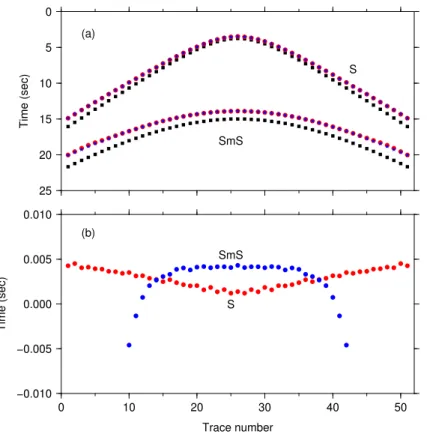
seismograms generated by an earthquake at 12.0 km depth in a homogeneous crust with a thickness of 30.0 km based on a high-order finite-difference method (in Ap-pendix). 51 surface stations with an equal spacing of 2.0 km are used to record seis-mograms.α=β=γ=1.0 are chosen in formula (16). Figure 1a–c shows theS wave arrival-time picking using the STA/LTA and EER methods on the seismogram for trace 10

number 26 (Fig. 1d). We can see thatS arrival time determined by the EER method is very close to the theoretical arrival time with errors smaller than 0.05 s. For the STA/LTA method, the threshold value is set to be 1.0×10−8, and the obtainedS arrival time is 0.24 s later than the theoretical arrival time. Note that an error of 0.24 s is unacceptable in traveltime inversion for local structures. We further show S and SmS arrival times 15

on all 51 seismograms in Fig. 1d. For directS wave, results of both STA/LTA and EER methods are relatively close to the theoretical arrival times, with errors around 0.3 s and less than 0.1 s, respectively. However, for SmS phase, the STA/LTA algorithm is not able to give accurate estimates on the breaking times. In comparison, the EER method gives picked arrivals with accuracy similar to the directSwave case, and 70 % 20

of the errors are still less than 0.1 s. We have fixed all parameters for the STA/LTA and EER methods in picking the S and SmS arrival times. Actually, the accuracy of time picking on any single seismogram can be improved by slightly tuning some parame-ters, such as the threshold value for the STA/LTA method and the lengths of the time windows for both methods. We also find that the accuracy of the STA/LTA method is 25

(15)

appropri-SED

6, 2523–2566, 2014

P. Tong et al.

Title Page

Tables Figures

◭ ◮

Back Close

Full Screen / Esc

Discussion

P

a

per

|

Discus

sion

P

a

per

|

Discussion

P

a

per

|

Discussion

P

a

per

|

ate threshold in practice. For the EER method, however, it is simple to locate the peak of the ratio functionr(t). This implies that the EER method could be a better choice for arrival-time picking on synthetic seismograms.

3.2 Combined ray and cross-correlation method

Because of the non-linearity of seismic inverse problems, seismic tomography usually 5

relies on an iterative method to find the optimal model. If the starting model m₀ for traveltime seismic tomography is simple (e.g., 1-D layered model) and travelling paths of particular phases can be easily traced, the arrival times T₀syn of synthetics in m₀ can be accurately determined based on ray theory. Meanwhile, we may expect that synthetic seismograms in the (i+1)th model m_i₊₁ are reasonably similar to those in 10

theith modelm_i (i≥0), and the arrival-time shiftδt_i₊1,i of a particular phase in models

m_i₊₁andm_i can be calculated with high accuracy by maximizing the cross-correlation formula,

max

δt_i₊_1,_i

RT

0w(τ)s(τ;mi+1)s(τ−δti+1,i;mi)dτ

h RT

0w(τ)s2(τ;mi+1)dτ

RT

0s2(τ−δti+1,i;mi)dτ

i1/2

, (17)

wherew(t) is the time window function used to isolate the interested phase (Liu et al., 15

2004). Consequently, the arrival timeT_isyn₊₁ of the synthetic seismogram in modelm_i₊₁ satisfies the following relation,

T_isyn₊₁ =T₀syn+

i

X

j=0

δt_j₊1,j. (18)

Since T₀syn and δtj+1,j are calculated with ray theory and cross-correlation method,

respectively, Eq. (18) is called the combined ray and cross-correlation method. 20

(16)

SED

6, 2523–2566, 2014

P. Tong et al.

Title Page

Tables Figures

◭ ◮

Back Close

Full Screen / Esc

Discussion

P

a

per

|

Discus

sion

P

a

per

|

Discussion

P

a

per

|

Discussion

P

a

per

|

be the crust model with an S wave velocity of 3.2 km s−1 and a thickness of 30.0 km.

Swave velocity inm₁is assumed to be 3.456 km s−1which has a perturbation of 8.0 % with respect to m₀. Synthetic seismograms generated by an earthquake at 12.0 km depth are calculated and recorded by 51 stations at the surface in bothm₀ and m₁. For modelsm₀andm₁, theoretical arrival times of S and SmS phases at each station 5

can be calculated based on the ray theory (see solid red circles and black squares in Fig. 2a). Based on Eq. (17), we also measure arrival shifts of S and SmS inm₁ from those inm₀. Adding S and SmS arrival shifts to their corresponding arrival times form₀ (solid black squares in Fig. 2a), we get the approximated arrival times of S and SmS in model m₁ (blue stars in Fig. 2a). Figure 2b shows the errors of the combined ray 10

and cross-correlation method in determining the arrival times of S and SmS in model m₁. It can be observed that the errors of direct S arrivals are less than 0.005 s, and 70 % errors of the SmS phases are smaller than 0.005 s with maximum error around about 0.175 s occurring at the 4th and 48th stations. Considering that the traveltime differences of the SmS phase in the two models are about 1.7 s at the two stations, 15

these picking errors are relatively small. This numerical example suggests that the combined ray and cross-correlation method could serve as an efficient tool for high accuracy arrival-time picking on synthetic seismograms in the iterative wave-equation based tomographic inversions.

4 Model Parameterization

20

Tomographic equation (13) needs invariably to be discretized for actual inversions (No-let et al., 2005). This gives rise to model parameterization, which is an approximation to the true Earth structure. Model parameterization determines the accuracy of forward modelling and hence affects the final form of tomographic inversion results. Most com-monly, functional approach with a set of basis functions or an a prior functional form, 25

(17)

SED

6, 2523–2566, 2014

P. Tong et al.

Title Page

Tables Figures

◭ ◮

Back Close

Full Screen / Esc

Discussion

P

a

per

|

Discus

sion

P

a

per

|

Discussion

P

a

per

|

Discussion

P

a

per

|

advantages and drawbacks (e.g. Zhao, 2009; Rawlinson et al., 2010). To guarantee accurate computation of synthetic seismograms and traveltime kernels and to adapt to local variations in data coverage, we use two sets of grid nodes (i.e., forward modelling grid and inversion grid) to parameterize the Earth structure for forward modelling and inversion algorithms in this study.

5

4.1 Forward modelling grid

As discussed in Sect. 2, we need to solve wave Eqs. (4) and (9) to obtain syn-thetic seismogramu(t) and traveltime kernelK(x). Many numerical methods such as staggered-grid finite-difference (FD) method (e.g. Virieux, 1984; Graves, 1996) and spectral-element method (Komatitsch and Tromp, 1999) are well suited for this kind 10

of forward modelling. In this study, we choose a FD scheme called high-order cen-tral difference method (see Appendix) to conduct forward modelling. The prominent feature of this high-order central difference method is that it simultaneously computes the displacement u(t,x) and the spatial gradient field ∇u(t,x), making the computa-tion of the traveltime kernel K(x) very straightforward. It is also easier to implement 15

the high-order central difference method than the staggered-grid finite-difference (FD) method and spectral-element method. When sensitivity kernels are calculated by solv-ing the full wave equation, there are spurious amplitudes in the immediate vicinity of the sources and receivers (Tape et al., 2007; Tong et al., 2014a). An efficient way of removing these spurious amplitudes is to smooth the traveltime kernelK(x)=K(x,z) 20

with a 2-D Gaussian

G(x,z)= 4

πσ2e

−4(x2+z2)/σ2_, ₍₁₉₎

(18)

SED

6, 2523–2566, 2014

P. Tong et al.

Title Page

Tables Figures

◭ ◮

Back Close

Full Screen / Esc

Discussion

P

a

per

|

Discus

sion

P

a

per

|

Discussion

P

a

per

|

Discussion

P

a

per

|

by

˜

K(x,z)=

Z Z

S

K(x−x′,z−z′)G(x′,z′)dx′dz′, (20)

i.e., the smoothed kernel value at a given point is obtained by averaging the un-smoothed kernel values at its neighbouring points.

For the 2-D FD numerical simulation, the continuous areaS is sampled by a set ofn

5

discrete nodesx_i (i =1, 2,· · ·,n). By choosing a corresponding set ofnbasis functions

Li(x) (i =1, 2,· · ·,n), the smoothed traveltime kernel ˜K(x) and the relative velocity

per-turbationδc(x)/c(x) can be expanded into linear combinations of the basis functions as

˜

K(x;x_r,x_s)=

n

X

i=1

K_iL_i(x) , δc(x)/c(x)=

n

X

i=1

C_iL_i(x), (21)

10

whereK_i andC_i are the corresponding coefficients related to the basis functionL_i(x). Substituting Eq. (21) into Eq. (13) results in the discrete form of the tomographic equa-tion

Tobs−Tsyn=

Z

S





n

X

j=1

K_jL_j(x)



 " _n

X

i=1

C_iL_i(x)

#

dx₌

n

X

i=1





n

X

j=1

K_j Z

Ω

L_j(x)L_i(x)dx



C_i. (22)

A general way to define a basis functionLi(x) is to construct a local interpolation

func-15

tion on knot nodex_i and its neighbours. The possibility of different choices for the basis functionsL_i(x) (i =1,· · ·,n) has led to various inversion algorithms (Nolet et al., 2005). As the high-order central difference method discussed in this study simulates seismic wave propagation on a 2-D regular mesh, we assume the spatial increments alongx

andzdirections are∆xand∆z, respectively. Let the knot nodex_i with a global indexi

(19)

SED

6, 2523–2566, 2014

P. Tong et al.

Full Screen / Esc

be the grid node (xm,zn) on the 2-D mesh. In this scenario, the simplest basis function

may be the piecewise constant function

L_i(x)=L_i(x,z)=

(

1, if (x,z)∈

x_m₋1/2,xm+1/2

×

z_n₋1/2,zn+1/2

;

0, else . (23)

And the coefficient of the unknownC_i in Eq. (22) is

n

X

j=1

K_j Z

Ω

L_j(x)L_i(x)dx_{= ∆}x∆zK_i. (24)

5

However, interpolation function with the basis functions (23) is not even continuous. To make the interpolation function continuous, we could use bilinear interpolation to fit the perturbation fieldδc(x)/c(x) and the traveltime kernelK(x). Bilinear interpolation performs linear interpolation first in one direction and then in the other direction. The basis functionL_i(x) for bilinear interpolation takes the following form

10

Li(x)=Li(x,z)=

              

x−xm−1

x_m−x_m₋₁ z−zn−1

z_n−z_n₋₁, if (x,z)∈

x_m₋1,xm

×

z_n₋1,zn

;

x−x_m₋₁ x_m−x_m₋₁

zn+1−z

z_n₊₁−z_n, if (x,z)∈

x_m₋1,xm

×[z_n,z_n₊1] ;

xm+1−x

xm+1−xm

z−zn−1

zn−zn−1, if (x,z)∈[xm,xm+1]×

zn−1,zn

;

x_m₊₁−x xm+1−xm

z_n₊₁−z

zn+1−zn, if (x,z)∈[xm,xm+1]×[zn,zn+1] ;

0, else .

(25)

Correspondingly, the coefficient for the unknownCi in Eq. (22) becomes

n

X

j=1

Kj

Z

Ω

Lj(x)Li(x)dx= ∆x∆z

  1 36 4 36 1 36 4 36 16 36 4 36 1 36 4 36 1 36  ◦  

K_m₋_1,_n₊₁ K_m_,_n₊₁ K_m₊_1,_n₊₁ Km−1,n Km,n Km+1,n

K_m₋1,n−1 Km,n−1 Km+1,n−1



(20)

SED

6, 2523–2566, 2014

P. Tong et al.

Title Page

Tables Figures

◭ ◮

Back Close

Full Screen / Esc

Discussion

P

a

per

|

Discus

sion

P

a

per

|

Discussion

P

a

per

|

Discussion

P

a

per

|

where ◦ denotes entrywise product and kernel values for global and local grids are linked by Ki+pM+q=Km+p,n+q (M is the number of grid nodes along x direction, and

p,q=−1, 0, 1). To have a smoother fitting function, we could further use bicubic inter-polation, which is an extension of cubit interpolation on 2-D regular mesh. Actually, in the framework of piecewise constant interpolation (Eq. 23), both bilinear interpolation 5

and bicubic interpolation can be achieved by replacingC_i’s coefficient∆x∆zK_i in Eq. (24) with a weighted average value∆x∆z_K˜_i _{around the knot node}_x_i_{and its neighbours} such as shown in Eq. (26). Since we have previously smoothed the kernel by convolv-ing it with a Gaussian, usconvolv-ing piecewise constant interpolation or bilinear interpolation to construct tomographic equation (22) is accurate enough for practical applications. 10

4.2 Inversion grid

For the high-order central difference scheme, we assume that seismic waves propagate in 2-D vertical planes and hence sensitivity kernels are restricted to the same 2-D planes. For a single pair of source x_s and receiver x_r, the forward grid nodes and equally the velocity model parametersCi are distributed on a 2-D regular mesh in Eq.

15

(22). An additional set of grid nodes needs to be introduced to characterize the actual 3-D tomographic region. For simplicity, we use a regular grid with variable grid intervals to represent the final tomographic results, which has the advantage of allowing a fine grid for a target volume with dense data coverage (mostly depending on spatial distribution of source and receivers) to be imbedded in coarse grid nodes.

20

To be consistent with the realistic application in the second paper, we directly set up the inversion grid in geographical coordinate system (d,φ,λ), where d, φ, and λ

are depth, latitude and longitude, respectively. If the Cartesian coordinate system is adopted for the inversion grid, the following derivation procedure is almost the same. In a 3-D regular inversion grid, each forward modelling grid nodex_i (i =1, 2,· · ·,n) is 25

(21)

SED

6, 2523–2566, 2014

P. Tong et al.

Full Screen / Esc

coordinate ˜x_i prior to locating it in a cube. Assume that ˜x_i is located within the cube formed by (d_r₊_j

1,φp+j2,λq+j3) (j1,j2,j3=0, 1; 1≤r+j1≤R; 1≤p+j2≤P; 1≤q+j3≤Q; R,P,Q are the numbers of inversion grid nodes along depth, latitude and longitude, respectively), the unknown velocity model parameter Ci corresponding to ˜xi can be

expressed as a linear combination of the parametersX_r₊_j

1,p+j2,q+j3 (j1,j2,j3=0, 1) at

5

the eight inversion grid nodes:

C_i = 1

X

j₁,j₂,j₃=0 1−

d−dr+j₁

d_r₊1−dr

! 1−

φ−φp+j₂

φ_p₊1−φp

! 1−

ψ−ψ_q₊_j 3 ψ_q₊1−ψq

X_r₊_j₁,p+j2,q+j3,

(27)

and defines a continuously varying velocity perturbation fieldδc(x)/c(x). Note that the velocity fieldc(x) itself can be discontinuous. Substituting Eq. (27) into Eq. (22) gives the tomographic equation on the inversion grid

10

Tobs−Tsyn=

R

X

r=1

P

X

p=1

Q

X

q=1

ar,p,qXr,p,q, (28)

wherear,p,q is the coefficient for the unknownXr,p,q and pre-determined, the accuracy

of which relies on not only the accurate calculation of the traveltime kernelK(x) but also the choice of the inversion grid. For the convenience of discussion, we convert the 3-D array index (r,p,q) of the inversion grid to 1-D indexn=(r−1)P Q+(q−1)P+q

15

(1≤n≤N=RP Q). Tomographic equation (28) can be rewritten as

Tobs−Tsyn=

N

X

n=1

a_nX_n (29)

for a single pair of source x_s and receiver x_r, which relates the traveltime residual

Tobs−Tsyn linearly to the unknown relative velocity perturbationX_n (1≤n≤N) on the inversion grid.

(22)

SED

6, 2523–2566, 2014

P. Tong et al.

Title Page

Tables Figures

◭ ◮

Back Close

Full Screen / Esc

Discussion

P

a

per

|

Discus

sion

P

a

per

|

Discussion

P

a

per

|

Discussion

P

a

per

|

5 Regularization and Inversion Method

With a significant increase in both quantity and quality of seismic data from the prolif-eration of dense seismic arrays, increasing number of seismic data will be involved in seismic tomography, which may result in higher-resolution tomographic models. Cer-tainly, more data will increase the complexity of seismic inverse problem.

5

When M seismic measurements are used to explore the subsurface structure, M

tomographic equations take the form of Eq. (29) and form a linear system b=AX at each iteration, where b₌[bm]M×1 and bm=Tmobs−T

syn

m is the iterative traveltime

residual vector,A=[a_m,n]M×N is the Fréchet or Jacobin matrix calculated in the current

iterative model andX=[Xn]N×1 is the unknown model vector. Since the problemb= 10

AX is always ill-posed (either because of non-uniqueness or non-existence ofX), the general way to solve it is to seek a solution that minimizes the following regularized objective function

χ(X)=1

2(AX−b)

T_C−1

d (AX−b)+

ǫ2

2 X

T_C−1 m X+

η2

2 X

T_DT_D_X_, ₍₃₀₎

whereCd and Cm are the a prior data and model covariance matrix which reflect the 15

uncertainties in the data and the initial model (Rawlinson et al., 2010),Dis a deriva-tive smoothing operator for model vectorX,ǫand ηare the damping parameter and smoothing parameter, respectively (e.g. Tarantola, 2005; Li et al., 2008; Rawlinson et al., 2010). The last two terms on the right hand side of Eq. (30) are regularization terms, which are included to improve the conditioning of the inverse problemb₌AX 20

and are designed to give preference to solutions with desirable properties (Aster et al., 2012): damping favours a result that is close to the reference model, while smooth-ing reduces the differences between adjacent nodes and thus produces smooth model variations (Li et al., 2006). Generally speaking, objective function (30) tries to strike a balance between how well the solution satisfies the data, the variations of the solu-25

(23)

SED

6, 2523–2566, 2014

P. Tong et al.

Title Page

Tables Figures

◭ ◮

Back Close

Full Screen / Esc

Discussion

P

a

per

|

Discus

sion

P

a

per

|

Discussion

P

a

per

|

Discussion

P

a

per

|

Calculating the gradient (Fréchet derivative) of the objective function χ(X) is often a key step in finding an optimal solution to the minimization problem (30) (Rawlinson et al., 2010). Here the Fréchet derivative of the objective function χ(X) can be ex-pressed as

∂χ(X)

∂X =

ATC−_d1A+ǫ2_C−1

m +η2DTD

X−ATC−_d1b. (31)

5

Based on the Fréchet derivative∂χ(X)/∂X, we describe two different approaches to solve the optimization (minimization) problem (Eq. 30).

5.1 LSQR solver

The minimizerX˜ of Eq. (30) satisfies∂χ(X˜)/∂X₌0 and formally can be expressed as 10

˜

X₌ATC_d−1A₊ǫ2C−_m1₊η2DTD−1ATC−_d1b. (32)

Clearly, to explicitly obtainX˜we need to invert anN×Nmatrix. There are various meth-ods available to fulfil this goal, such as LU decomposition, single value decomposition (SVD), conjugate-gradient type of methods such as LSQR algorithm. Among these methods, LSQR algorithm may be one of the most efficient and widely used methods 15

to solve a linear system, especially whenN is very large (Paige and Saunders, 1982). Additionally, the minimization problem (Eq. 30) is equivalent to solving the following linear system in a least square sense



 

C−_d1/2A ǫC−_m1/2

ηD 



X=



 

C−_d1/2b

0 0





, (33)

and application of LSQR or SVD to Eq. (33) will give the same solution as that of Eq. 20

(24)

SED

6, 2523–2566, 2014

P. Tong et al.

Title Page

Tables Figures

◭ ◮

Back Close

Full Screen / Esc

Discussion

P

a

per

|

Discus

sion

P

a

per

|

Discussion

P

a

per

|

Discussion

P

a

per

|

model can be updated from the current velocity model on inversion grid,C, toC+X˜. Because of the non-linearity of the inverse problem, further iteration may be needed to update the velocity model until the objective functionχ(X) reaches below a tolerance level.

5.2 Non-linear conjugate gradient method

5

Once we have the Fréchet derivative of the objective function computed in Eq. (31), instead of inverting the matrix in Eq. (32), we can alternatively use a non-linear conjugate-gradient method to iteratively improve the model (e.g. Fletcher and Reeves, 1964; Tromp et al., 2005). Previous studies have shown the feasibility and efficiency of this non-linear conjugate-gradient method in recovering seismic properties of the Earth 10

interior (e.g. Tape et al., 2007, 2009; Zhu et al., 2012). Here we summarize the step-by-step process of this non-linear conjugate-gradient method, which starts fromk=0 (Tape et al., 2007; Kim et al., 2011):

1. Calculate the objective functionχ(Xk), compute the gradientgk₌∂χ /∂Xk,

2. Compute the model update direction pk=−gk+βkpk−1. For the first iteration

15

k=0, setβ0=0 andp 0

=−g0; otherwise calculateβ_k based on the formula

β_k=max 0,g

k

·(gk−gk−1) gk−1_·_gk−1

!

. (34)

3. Determine the step lengthλ_k in the model update direction:

– Letf1=χ(X

k

),g1=g

k

·pk, and compute a test step lengthλt=−2f1/g1.

– Calculate the test perturbation modelXk_t ₌Xk₊λtpk.

20

– Compute the objective functionχ(Xk_t) and letf2=χ(Xkt). Note that we

(25)

SED

6, 2523–2566, 2014

P. Tong et al.

Title Page

Tables Figures

◭ ◮

Back Close

Full Screen / Esc

Discussion

P

a

per

|

Discus

sion

P

a

per

|

Discussion

P

a

per

|

Discussion

P

a

per

|

– Compute

γ=[(f2−f1)−g1λt]/λ2t, ξ=g1 (35)

and thenλ_kis given by

λ_k=

(

−ξ/(2γ), γ6=0;

error, otherwise. (36)

4. Update the perturbation modelXk+1₌Xk₊λ_kpk. 5

5. If||gk||L₂=(gk·gk)1/2≤ǫ, the tolerance level, thenXk+1is the optimal

perturba-tion model; otherwise reiterate from the first step (i) withk+1.

For the current modelm_kwhich has a perturbationXk from the starting modelm₀, we can rewrite the gradient of the objective function as

∂χ(Xk)

∂X =−(A

k₎T_C−1

d b k

+ǫ2C−_m1+η2DTDXk, (37) 10

whereAkandbkare respectively the Fréchet matrix and traveltime residuals in thekth model. The first term on the right hand side of Eq. (37) is actually the sum of all trav-eltime kernels (negatively) weighted by their corresponding travtrav-eltime residuals. That is to say, if no damping and smoothing operations are applied, the gradient (Eq. 37) is simply the sum of all weighted individual traveltime kernels. Since operatorsC−_d1,C−_m1

15

andDremain constant throughout the whole process, to update the model fromm_k to m_k₊₁ we only need to compute the Fréchet matrix and traveltime residuals in model m_k. This is different from the approach using the LSQR algorithm as a linear system is solved at each iteration. Generally speaking, the model update with the LSQR al-gorithm may be larger than the non-linear conjugate-gradient method and the LSQR 20

(26)

SED

6, 2523–2566, 2014

P. Tong et al.

Title Page

Tables Figures

◭ ◮

Back Close

Full Screen / Esc

Discussion

P

a

per

|

Discus

sion

P

a

per

|

Discussion

P

a

per

|

Discussion

P

a

per

|

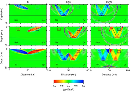
6 Numerical examples

As discussed in Sect. 5, computing traveltime sensitivity kernel or the Fréchet deriva-tive of the objecderiva-tive function is one of the key components of wave-equation based traveltime seismic tomography. In this section, we show examples of Fréchet kernel for one earthquake. These examples provide insights into sensitivities of various seismic 5

phases and the future applications of wave-equation based traveltime seismic tomog-raphy involving tens of thousands of seismic records.

A two-layerS wave velocity model with the Moho discontinuity at a depth of 30.0 km is used as a reference model. The size of the model is 100 km×50 km. S wave ve-locities in the crust and the mantle are 3.2 km s−1 and 4.5 km s−1, respectively. The 10

“true” model is the same two-layer S wave velocity model but with a −5.0 % low ve-locity anomaly (red box in Fig. 5) and a +5.0 % high velocity anomaly (blue box in Fig. 5) included in the mid-crust. An earthquake is placed at the horizontal distance

x=50.0 km and the depth of 12.0 km with the dominant frequency of the Gaussian source time function at 1.0 Hz. There are 51 stations equally spaced on the surface 15

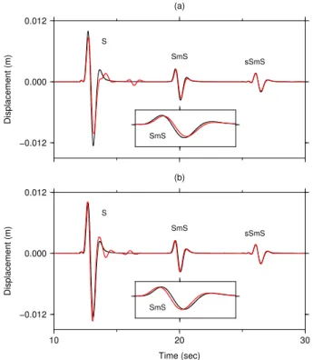
with an interval of 2.0 km. The high-order central difference method is used as the for-ward solver. Seismograms recorded atx=14.0 km andx=86.0 km on the surface are shown in Fig. 4a and 4b, respectively. Three main phases can be observed in these seismograms, including the directS wave, the Moho reflected phase SmS and the sur-face reflected wave sSmS, which provide complementary information on the crustal 20

structures. For example, D. Zhao et al. (2005) have used S, SmS and sSmS arrivals to conduct crustal tomography in the 1992 Landers earthquake area with a ray-based tomographic method. Here we compute Fréchet kernels for the three seismic phases. Because only sensitivity kernels are computed and no inversion is conducted, the two regularization terms at the right hand side of Eq. (37) are not taken into account in this 25

section.