IAEES www.iaees.org Article
Six (arguably) necessary steps forwards in landscape connectivity
and genetics
Alessandro Ferrarini
Department of Evolutionary and Functional Biology, University of Parma, Via G. Saragat 4, I-43100 Parma, Italy E-mail: [email protected], [email protected], [email protected]
Received 2 November 2016; Accepted 10 December 2016; Published online 1 March 2017
Abstract
Landscape heterogeneity and fragmentation affect how organisms are distributed in the landscape, determine the chance of a patch being colonized, reduce inbreeding in small populations and maintain evolutionary
potential. Predicting the way in which animals disperse is pivotal for management and conservation purposes. I discuss here the conceptual and methodological weak points of circuit theory and least-cost modelling, the two most commonly-used methods in the scientific literature. I argue that these two methods, although very
brilliant and very well supported by freely-available softwares, make use of six axiomatic assumptions: 1) any landscape can be divided into source and sink areas for any considered species; 2) source-sink areas can be a priori defined by the users; 3) any species adopt a global optimization of its dispersal over any landscape; 4) biotic movements are undirected; 5) stability points along dispersal paths are absent; 6) frictional values based
on expert opinion are true-to-life. I argue that these axioms are only realistic for a limited number of species with short-range shifts over lowland (or, at least, patchy) landscapes, and for which frictional values can be realistically defined. I also describe an alternative theoretical and methodological approach, called Flow
Connectivity, which can fix such weak points.
Keywords biotic movements; dispersal modelling; Flow Connectivity; gene flow; landscape connectivity;
landscape genetics; simulation models; species conservation; species management.
1 Introduction
Landscape connectivity was initially introduced as “the degree to which the landscape impedes or facilitates movements among resource patches” (Taylor et al., 1993). Due to the difficulty in collecting experimental results on species dispersal, simulation models have become a cost-effective approach to predict dispersal dynamics (Tischendorf, 1997; Tischendorf and Fahrig, 2000). Simulation models with spatially-explicit
landscapes enable the integration of the relationships between species and landscapes, and provide Environmental Skeptics and Critics
ISSN 22244263
URL: http://www.iaees.org/publications/journals/environsc/onlineversion.asp
RSS: http://www.iaees.org/publications/journals/environsc/rss.xml
Email: [email protected]
EditorinChief: WenJun Zhang
representation of the spatial elements that promote or constrain dispersal. Several dispersal models with spatially-explicit landscapes have been developed (Gustafson and Gardner, 1996; Gardner and Gustafson,
2004). The two most commonly-used methods in the recent scientific literature are circuit theory (McRae, 2006; McRae and Beier, 2007; McRae et al., 2008) and least-cost modelling (Dijkstra, 1959).
In circuit theory (CT from now on), landscapes are represented as conductive surfaces, with resistance
proportional to the easiness of species dispersal or gene flow. Low resistances are assigned to habitats that are most permeable to movement or that best promote gene flow, and high resistances are given to poor dispersal
habitats and barriers. Circuit theory offers several advantages, including a theoretical basis in random walk theory and the ability to evaluate contributions of multiple dispersal pathways.
Least-cost modelling (LC hereafter) is an algorithm that computes a deterministic trajectory (also termed
least cost path; LCP hereafter) between a start and an end point moving along a frictional landscape. A LCP minimises the sum of frictions of all pixels along the path. Least-cost modelling is an attractive technique for
analysing and designing habitat corridors because it: 1) allows quantitative comparisons of potential movement routes over large study areas, 2) can incorporate simple or complex models of habitat effects on movement and 3) offers the potential to escape the limitations of analyses based solely on structural connectivity (i.e.
designating areas as patch, matrix or corridor) by modelling connectivity as it might be perceived by a species on a landscape.
Hundreds of papers in the recent scientific literature present applications of these two methodologies. I examine here six conceptual and methodological weak points of CT and LC. I argue that the use of these two
methodologies, although very brilliant and very well supported by freely-available softwares, can only be realistic for a limited number of species with short-range shifts over lowland landscapes, and for which frictional values can be realistically defined. I also describe an alternative solution called Flow Connectivity
which fixes these six weak points.
2 Three Conceptual Weak Points in Circuit Theory and Least-Cost Modelling 2.1 Is the source-sink approach realistic?
In CT and LC, species dispersals are thought as “from-to” movements, i.e. from source points (landscape
patches) to sink ones. Sources and sinks are suitable areas present within a landscape matrix that is partially, or completely, hostile to the species. It easily follows that both CT and LC are suitable for application to patchy
landscapes that can present source and sink areas. But, what kinds of landscapes present this attribute? Mountain and hilly landscapes are not composed of source and sink habitats, instead they’re a continuum composed of a natural matrix where the source-sink approach loses its rationale. A source-sink model can only
be suitable to describe landscapes where suitable patches (e.g., protected areas or remnant natural patches) are surrounded by a dominant, hostile (or semi-hostile) anthropogenic landscape. Thus only lowland (or, at least,
patchy) landscapes can properly meet the requirements of CT and LC, while the application of these two methodologies to different kinds of landscapes is a priori incorrect from a conceptual viewpoint.
2.2 Can source-sink patches be realistically defined a priori by the user?
Both CT and LC require to a priori define source and sink points/patches of the landscape under study. This is the typical case of expert opinion, which represents a top-down approach to the problem. But, isn’t this an
2.3 Is the global optimization of dispersal paths realistic?
CT and LC assume that species travel from starting patches towards stopping ones. This assumption involves
that each species is supposed to a priori globally plan its path, otherwise stated: 1) dispersers have complete knowledge of their surroundings, 2) they do select the fittest route from this information. In fact, in case of local optimization of the dispersal path, the destination points are unknown to the species which only locally
can resolve the successive steps of its dispersal.
This kind of “global optimization” of the dispersal paths is a very strong assumption. It could result true for
short-range dispersals where the destination point is visible from the starting one, but for wide-range shifts the global optimization is, in most cases, untrue, unproven or, at least, very challenging to be demonstrated. For this simple reason, the global optimization of the dispersal paths should not be axiomatically assumed as true
by CT and LCP.
3 Three Methodological Weak Points in Circuit Theory and Least-Cost Modelling 3.1 Is the lack of directionality of dispersal paths realistic?
In CT and LC, pixel-level resistance to biotic flows is considered constant regardless of the dispersal direction.
While each pixel can be travelled in any direction, its friction value remains the same. This could be realistic for very accurate frictional maps where each pixel is supposed to be spatially homogeneous since it represents
a very small portion (e.g., 100*100 sq meter) of the study area, but it is inappropriate for frictional maps where each pixel represents large areas (e.g., 1 km * 1 km). Let’s think, for instance, to mountain or hilly landscapes where steep slopes determine local abrupt changes to the terrain direction. Going upslope or downslope is
completely different in such landscape since it locally imposes clear privileged/underprivileged directionalities to biotic flows. It easily follows that the directionality of biotic shifts can’t be omitted in realistic simulations
of species dispersal.
3.2 Is the absence of stability points/areas along the dispersal paths realistic?
CT and LC do not take into account the chance that dispersal paths can be interrupted at any point in case one
species detects a very suitable area other than the one a priori imposed by the user. Let’s suppose that, while travelling from the starting patch to the stopping one, a species finds a very suitable area for its persistence. Is
it realistic that such species will continue its dispersal towards the a priori-decided stopping point, as required by CT and LC? Is it realistic that one species resigns from a suitable area and makes a further (not costless)
effort in order to get another suitable area? Isn’t it more realistic that the presence of highly suitable habitats along the dispersal path determine stability points, and thus the interruption of species dispersal?
3.3 Is the expert opinion in frictional values assignment realistic?
CT and LC make use of frictional values based on expert opinions. By the way, how can we be sure that such values are realistic? In fact, in case of unrealistic frictional values, the resulting CT and LC simulations
become unrealistic as a logical and direct consequence.
CT and LC do not provide a sensitivity analysis of frictional values, so how can we assess the degree of uncertainty associated to the predictions of species dispersals and landscape connectivity? What is more, how
can we build up realistic frictional values for those species whose suitability for land cover classes is uncertain or unknown?
4 An Alternative Approach: Flow Connectivity
Flow connectivity (FC hereafter) is a methodology first introduced in 2013 (Ferrarini, 2013) to forecast biotic
Flow connectivity has been conceived to fix the six weak points of CT and LC described above. Its name is due to the fact that it resembles in some way the motion characteristic of fluids over a surface. In fact, FC
predicts species dispersal by minimizing at each time step the potential energy due to fictional gravity force over a frictional 3D landscape built upon the real landscape.
FC considers connectivity to be a function of a continuous gradient of permeability values rather than
attempting to distinguish discrete patches based on subjective thresholds. A comparison with CT and LC are discussed in Ferrarini (2013) and Ferrarini (2014d). At present FC presents many variants (Table 1), each
devoted to a particular topic of species dispersals over landscape.
Table 1 Flow Connectivity and its developed variants, each with a particular purpose.
Name Purpose Year Reference
Flow Connectivity Predicting biotic flows over landscape 2013 Ferrarini A. 2013
Reverse Flow Connectivity Assigning true-to-life friction values to biotic flows 2014 Ferrarini A. 2014
Backward Flow Connectivity Tracing biotic dispersals back in time 2014 Ferrarini A. 2014b
Sloping Flow Connectivity Detecting barriers and facilities to species dispersal 2014 Ferrarini A. 2014c
Bottleneck Flow Connectivity Detecting landscape bottlenecks of species dispersal 2015 Ferrarini A. 2015
Climatic Flow Connectivity Incorporating climatic change into biotic connectivity 2015 Ferrarini A. 2015b
What-if Flow Connectivity Integrating landscape changes into biotic connectivity 2015 Ferrarini A. 2015c
Momentum Flow Connectivity Mapping landscape impulses to species dispersal 2015 Ferrarini A. 2015d
Stochastic Flow Connectivity Associating uncertainty to biotic flows prediction 2016 Ferrarini A. 2016
Linkage Flow Connectivity Detecting the true corridors of species dispersal 2016 Ferrarini A. 2016b
4.1 A solution to the source-sink approach
FC does not necessitate to subdivide the landscape under study into source and sink points/patches. FC just
requires the frictional landscape built upon the real landscape (Fig. 1). For this reason it can be applied indifferently and realistically to lowland, hilly and mountain landscapes. The frictional landscape is built upon both structural and functional properties of the real landscape. In fact, if only structural aspects (typically, the
land cover map) are considered, the resulting frictional landscape would result in large, unrealistic clusters of homogeneous friction values. Instead, the use of multiple structural (e.g., elevation a.s.l., slope aspect, slope
acclivity) and functional (e.g., distance from water, distance from roads) predictors gives realistic gradient maps.
4.2 A solution to the a priori definition of source and sink patches
Fig. 1 Fictional landscape built for wolf upon a portion of the Ceno Valley (province of Parma, Italy). The elevation represents the landscape friction for the species under study: the higher the elevation, the higher the friction to the species. Black points represent sites where the species is simulated to be present. The image is borrowed from Ferrarini (2013).
Fig. 2 In red, theexpected dispersal paths of Canis lupus from simulated points of presence (black points) over the frictional
landscape of Fig. 1. The image is borrowed from Ferrarini (2013).
4.3 A solution to the global optimization of dispersal paths
FC uses a greedy, local-effort minimization for species dispersal that does not necessarily correspond to the
global minimization. As a result, it predicts dispersal paths that are much more complex and realistic than those produced by models that instead seek global optimization. In Fig. 3 the application of locally-optimized
Fig. 3 3D representationof the detected corridors for the frictional landscape of Fig. 1. Corridors are in different levels of green depending on the degree of biotic flow. Red areas are partially or totally unsuitable areas for biotic flows. The image is borrowed from Ferrarini (2016b).
4.4 A solution to the lack of directionality in species dispersal
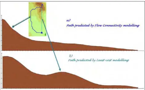
FC makes use of a clear directionality (directed movement) for predicting dispersal paths. At any position in the frictional landscape, a movement is possible only in the direction that mostly lowers the friction to the
species (Fig. 4). Instead CT and LC modeling have not a direction, in fact if one inverts the starting with the stopping point he achieves the same results (undirected movement).
Fig. 4 3D profile of the predicted biotic shift over the frictional landscape using flow connectivity (top) and least cost modelling
4.5 A solution to the absence of stability points in species dispersal
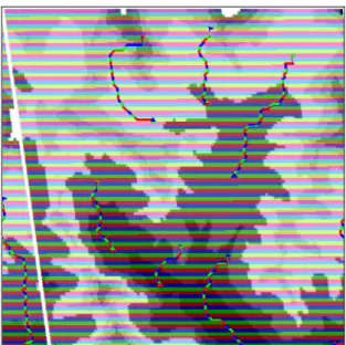
FC assumes that species dispersal ends at a stability point, if exists, that cannot be a priori defined by the user. A stability point exists when one species finds itself in a portion of the frictional landscape where all the surrounding pixels have equal or higher frictional values (Ferrarini 2013). When this happens, FC assumes that the species has no reason to move further (Fig. 5).
Fig. 5 Starting points (flags), predicted paths (red lines) and predicted stopping points (triangles) of dispersal paths using flow
connectivity. The image is borrowed from Ferrarini (2014d).
4.6 A solution to the subjectivity in frictional values assignment
True-to-life coefficients are calculated in FC as described in Ferrarini (2014). Using genetic algorithms, FC
builds up a frictional landscape so that real dispersal paths, detected using GPS or field observations, match perfectly the ones simulated by FC (Fig. 6). This bottom-up approach does not require expert opinion.
Fig. 6 The expected dispersal path from simulated presence (black point) is in red. The path in magenta represents the path
detected via GPS data-loggers. The area between the two curves represents the prediction bias B. Reverse flow connectivity aims
In addition, FC provides sensitivity analyses of frictional values (Ferrarini, 2016). FC is applied through the ad hoc software Connectivity-Lab 2.6 (Ferrarini, 2013b). Table 2 provides a synthetical comparison among FC, CT and LC.
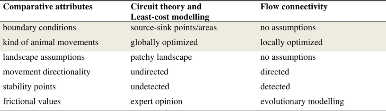
Table 2 A comparative synthesis of the attributes of circuit theory, least-cost modelling and flow connectivity.
Comparative attributes Circuit theory and
Least-cost modelling
Flow connectivity
boundary conditions source-sink points/areas no assumptions
kind of animal movements globally optimized locally optimized
landscape assumptions patchy landscape no assumptions
movement directionality undirected directed
stability points undetected detected
frictional values expert opinion evolutionary modelling
5 Conclusions
Circuit theory and least-cost modelling, although very brilliant and very well supported by freely-available
softwares, make use of six axiomatic assumptions about species dispersal and landscape connectivity. As discussed above, these axioms can be realistic for a limited number of species with short-range shifts over lowland (or, at least, patchy)landscapes, and for which frictional values can be realistically defined. The use of
CT and LC for different conditions is at risk of producing biased, or at least unreliable, predictions of species dispersals over landscapes.
FC represents an alternative approach to CT and LC, which fixes the above-depicted weak points. FC does not require to know in advance source-sink points/areas, and it does not presume that dispersers are able to globally optimize their dispersal paths. In addition, FC allows for directionality of biotic flows, and for the
presence of stability points along the dispersal paths. Last, frictional values are assessed via evolutionary modelling, and sensitivity analyses provide further information about the possible degree of indecision.
References
Dijkstra EW. 1959. A note on two problems in connexion with graphs. Numerische Mathematik, 1: 269-271 Ferrarini A. 2013. A criticism of connectivity in ecology and an alternative modelling approach: Flow
connectivity. Environmental Skeptics and Critics, 2(4): 118-125
Ferrarini A. 2013b. Connectivity-Lab 2.6: a software for applying connectivity-flow modelling. Manual, 104 pages (in Italian)
Ferrarini A. 2014. True-to-life friction values in connectivity ecology: Introducing reverse flow connectivity. Environmental Skeptics and Critics, 3(1): 17-23
Ferrarini A. 2014b. Can we trace biotic dispersals back in time? Introducing backward flow connectivity. Environmental Skeptics and Critics, 3(2): 39-46
Ferrarini A. 2014c. Detecting barriers and facilities to species dispersal: introducing sloping flow connectivity.
Proceedings of the International Academy of Ecology and Environmental Sciences, 4(3): 123-133
Ferrarini A. 2014d. Ecological connectivity: Flow connectivity vs. least cost modelling. Computational
Ferrarini A. 2015. Where do they come from? Flow connectivity detects landscape bottlenecks. Environmental Skeptics and Critics, 4(1): 27-35
Ferrarini A. 2015b. Incorporating climatic change into ecological connectivity: Climatic Flow Connectivity. Computational Ecology and Software, 5(1): 63-68
Ferrarini A. 2015c. Integrating landscape changes into ecological connectivity: What-if flow connectivity.
Proceedings of the International Academy of Ecology and Environmental Sciences, 5(2): 77-82
Ferrarini A. 2015d. Mapping landscape impulses to species dispersal: Momentum Flow Connectivity.
Environmental Skeptics and Critics, 4(3): 81-88
Ferrarini A. 2016. Associating uncertainty to the prediction of biotic flows: Stochastic Flow Connectivity. Computational Ecology and Software, 6(1): 12-20
Ferrarini A. 2016b. Detecting and weighting the true corridors of biotic shifts and gene flows: Linkage Flow Connectivity. Environmental Skeptics and Critics, 5(2): 28-36
Gardner RH, Gustafson EJ. 2004. Simulating dispersal of reintroduced species within heterogeneous landscapes. Ecological Modelling, 171: 339-358
Gustafson EJ, Gardner RH. 1996. The effect of landscape heterogeneity on the probability of patch
colonization. Ecology, 77: 94-107
McRae BH. 2006. Isolation by resistance. Evolution, 60: 1551-1561
McRae BH, Beier P. 2007. Circuit theory predicts gene flow in plant and animal populations. Proceedings of the National Academy of Sciences of the USA, 104: 19885-19890
McRae BH, Dickson BG, Keitt TH, Shah VB. 2008. Using circuit theory to model connectivity in ecology and conservation. Ecology, 10: 2712-2724
Taylor PD, Fahrig L, Henein K, Merriam G. 1993. Connectivity is a vital element of landscape structure.
Oikos, 68: 571-573
Tischendorf L. 1997. Modelling individual movements in heterogeneous landscapes: potentials of a new
approach. Ecological Modelling, 103: 33-42