Influence of climate, fire and phosphorus in the dynamics of vegetation in the Amazon-Cerrado border simulated with INLAND model

(1)

INFLUENCE OF CLIMATE, FIRE AND PHOSPHORUS IN THE DYNAMICS OF VEGETATION IN THE AMAZON-CERRADO BORDER SIMULATED

WITH INLAND MODEL

Dissertação apresentada à Universidade Federal de Viçosa, como parte das exigências do programa de Pós-Graduação em Meteorologia Aplicada, para obtenção do título de Magister Scientiae.

VIÇOSA

(2)

(3)

(4)

(5)

AGRADECIMENTOS

A Deus por me capacitar a cada dia e por me fazer ter a certeza de que tudo está sob Seu controle, por me dar paciência e cuidar de mim.

À minha família, por todo amor e por todo investimento a mim concedido, pelos valores morais e éticos ensinados cuidadosamente ao longo da minha vida. Eu amo demais vocês.

A meu querido Fernando Carvalho por todos os minutos de atenção, por todo amor e esforço realizado para estar junto de mim nesses dois anos. Por cada conselho amigo e palavra de ânimo nas longas ligações noturnas e por todos os abraços quentinhos nas chegadas aos sábados de manhã.

Ao professor Marcos Heil Costa por me receber tão bem e acreditar no meu potencial, por me dar a oportunidade de trabalhar em um grupo de excelência como o Grupo de Pesquisa em Interação Atmosfera-Biosfera. Ao professor Júlio Cesar Lima Neves por me coorientar, e me ensinar pacientemente essa ciência tão nova para mim que é a ciência de solos.

À Universidade Federal de Viçosa e ao Departamento de Engenharia Agrícola por me dar a oportunidade de desenvolver esse trabalho, não só pelo espaço físico, mas por todos os ensinamentos transmitidos.

À Fundação de Amparo à Pesquisa do estado de Minas Gerais (Fapemig), pela concessão da bolsa de estudos.

(6)

Aos meus amigos do Grupo de Pesquisa em Interação Atmosfera-Biosfera - Ana Beatriz, Carla Camargos, Matheus Lucas, Gabriel Abrahão, Gabrielle Pires (Gabis), Lívia Cristina, Patrícia Porta Nova, Victor Benezoli, Francisca Zenaide, Fabiana Couto (Fabi), Vítor Fontes, Fernando Pimenta, Telmo Sumila, Angélica Patarroyo e Pauline pela disponibilidade em ajudar sempre (principalmente com meus scripts e senhas que

sempre somem ou travam), pelos “cafés” e principalmente pela amizade.

Aos meus amigos e colegas do INPE o qual sempre foram atenciosos e solidários ao longo desta caminhada, auxiliando quando necessário nos aspectos pessoais e profissionais.

A nossa secretária Graça, por sua eficiência e carinho.

As minhas amigas de república, Mayana, Naysa, Glenda, Helen, Fernanda, Priscila pela amizade, pelo convívio, pela paciência e por transformarem nossa casa em

(7)

BIOGRAFIA

EMILY ANE DIONIZIO DA SILVA, filha de Gercilane Fonseca Dionizio da Silva e Cesar Henrique da Silva, nasceu em 09 de agosto de 1989 na cidade de Guaratinguetá, no estado de São Paulo. Em Fevereiro de 2006 ingressou no curso de Ciências Biológicas nas Faculdades Integradas Teresa D´Ávila (FATEA).

Em 2009 iniciou sua iniciação científica no Instituto Nacional de Pesquisas Espaciais (INPE) no Centro de Ciência do Sistema Terrestre (CCST) na cidade de Cachoeira Paulista, São Paulo, por onde atuou durante os dois anos pós-graduada.

(8)

CONTENTS

LIST OF SYMBOLS ... viii

LIST OF FIGURES ... ix

LIST OF TABLES ... xi

LIST OF ACRONYSMS ... xii

ABSTRACT ... xiv

RESUMO ... xvi

GENERAL INTRODUCTION ... 1

CHAPTER 1 ‒ Phosphorus in the soil and plants ‒ development of a phosphorus regional dataset ... 5

1.1 INTRODUCTION ... 5

1.2 MATERIALS AND METHODS ... 8

1.2.1Data Description of phosphorus in soil ... 8

1.2.2Description of the phosphorus regional data ... 8

1.2.3Estimating Ptotal from P-Mehlich-1 ... 12

1.2.4 Development and description of the phosphorus regional dataset (PR) ... 15

1.2.5 Description of the global phosphorus dataset (PG) ... 16

1.2.6 Development of Vmax regional and global datasets ... 17

1.3 RESULTS ... 19

1.3.1 Estimates of total phosphorus ... 19

1.3.2 Main differences between phosphorus datasets used in this study ... 21

1.3.3 Vmax maps used in this study ... 22

1.4 CONCLUSIONS ... 24

CHAPTER 2 – Effects of climate, fire and phosphorus in the Amazon-Cerrado border simulated with INLAND model ‒ Numeric experiment development ... 25

2.1 INTRODUCTION ... 25

2.2 MATERIALS AND METHODS ... 28

2.2.1Description of the INLAND Surface Model ... 28

2.2.2Model Configuration and Experiment Design ... 31

2.2.3 Analysis of the Model Sensitivity... 33

2.2.4Determination of the best model configuration ... 35

2.2.5Development of the MODIS LAI Map ... 35

2.2.6 Statistical Analyses ... 36

(9)

2.3.1 Comparison of simulations (Isolated Effects) ... 37

2.3.1.1 Climate effects ... 37

2.3.1.2 Phosphorus effect ... 42

2.3.1.3 Fire Effect ... 45

2.3.3 Longitudinal gradient of biomass and leaf area index in the Amazonia-Cerrado transition ‒ Comparison between simulations and field observations ... 50

2.3.4 Simulated composition of vegetation ... 54

2.4 CONCLUSIONS ... 60

3. GENERAL CONCLUSIONS ... 62

4. REFERENCES ... 64

(10)

LIST OF SYMBOLS

C Carbon

cm Centimeter

m Meters

m2 m-2 Square meter per square meter mm yr-1 _{Millimeter per year}

mg Milligram

mg L-1 Milligram per liter

mg dm-3 Milligram per cubic decimeter mg kg-1 Milligram per kilogram

μmol Micromolar m² Square meter

s Seconds

P Phosphorus

N Nitrogen

kg Kilogram

kg m-2 Kilogram per square meter

(11)

LIST OF FIGURES

(12)

(13)

LIST OF TABLES

(14)

LIST OF ACRONYSMS

C Clay

BESM Brazilian Earth System Model

CA Average climate (climatology 1961-1990) CENTURY Model of plant-soil nutrient cycling CLM The Community Land Model

CMAP Maximum capacity of the soil adsorption

CO2 Carbon Dioxide

CTEM Canadian Terrestrial Ecosystem Model CV Variable climate (database 1948-2008) DGVMs Dynamic Global Vegetation Models

F Fire

GPP Gross primary productivity HCL Hydrochloric acid

IBIS Integrated BIosphere Simulator

IGBP International Global Biosphere Programme INLAND Integrated Model of Surface Process

ISAM Integrated Science Assessment Model

JPL Lund-Potsdam-Jena Dynamic Global Vegetation Model LAIupper Upper canopy leaf area index

LAIlower Lower canopy leaf area index

LAIdry Dry season leaf area index (MODIS) LSM Land Surface Model

MODIS Moderate Resolution Imaging Spectroradiometer NPP Net primary production

P-Mehlich-1 Phosphorus extracted by Mehlich-1 extractor

P_m1_est Estimated Phosphorus extracted by Mehlich-1 extractor PAdc Phosphorus added in each soil sample

(15)

Presin Phosphorus extracted by Resin Ptotal Phosphorus total in the soil

Rubisco Ribulose-bisfosfato carboxilase oxigenase UNEMAT State University of Mato Grosso

Vmax Maximum rate of carboxylation Rubisco

(16)

ABSTRACT

SILVA, Emily Ane Dionizio da, M. Sc. Universidade Federal de Viçosa, February, 2015. Influence of climate, fire and phosphorus in the dynamics of vegetation in the Amazon-Cerrado border simulated with INLAND model. Adviser: Marcos Heil Costa. Co-Adviser: Júlio Cesar Lima Neves.

(17)

(18)

RESUMO

SILVA, Emily Ane Dionizio da, M. Sc. Universidade Federal de Viçosa, Fevereiro de 2015. Influência do clima, fogo e fósforo na dinâmica da vegetação na fronteira Amazônia-Cerrado simulada pelo modelo INLAND. Orientador: Marcos Heil Costa. Coorientador: Júlio Cesar Lima Neves

Estudos realizados para avaliar os principais fatores responsáveis pela dinâmica da vegetação na Amazônia tais como clima e/ou desmatamento sugerem a possibilidade da floresta Amazônica não resistir a uma eventual mudança do regime de chuvas, e ser transformada em um ecossistema de vegetação mais esparsa, do tipo savana, o que deu

origem ao termo “Savanização da Amazônia”. Parte destes estudos iniciais no entanto

(19)

(20)

GENERAL INTRODUCTION

On a global scale, the distribution of different forms of existing vegetation is in general controlled by the climate where the relations between precipitation and temperature determine the structural patterns of vegetation (Whittaker, 1975). At a regional level however, these structural patterns of vegetation can still depend on local environmental conditions imposed by local variations in soils, and topography.

The boundaries between the Amazon forest and the Brazilian Cerrado, for example, are not only characterized by a seasonal rainfall gradient, but also influenced in large part by the occurrence of fire, availability of water and nutrients in the soil, herbivory and soil characteristics (Lehmann et al., 2011; Murphy and Bowman, 2012; Sankaran et al., 2004). Due to the impossibility of manipulating some of these factors in their natural environments, it is difficult to assess and quantify the degree of interaction between these various factors and to infer how each of them works on the regional vegetation. Therefore, Dynamic Global Vegetation Models (DGVMs) have been used to isolate and manipulate factors like climate, fire and nutrients, to understand the large-scale effects of these factors on vegetation (Favier et al., 2004; Hirota et al., 2010; House et al., 2003).

(21)

2007) or tends towards a seasonal forest (Malhi et al., 2009). These pioneering studies were of paramount importance to the advancement of terrestrial biosphere modeling, but in general, the models commonly used by the scientific community have more realistic representations of temperate and cold climate ecosystems, rather than tropical ecosystems. In tropical regions, the DGVMs neglected important factors such as the effects of fire and nutritional limitations.

(22)

al., 2009; Paoli et al., 2008; Reich et al., 1995; Silver et al., 1994; Wang et al., 2010). Phosphorus is a nutrient that has not been incorporated in most of DGVMs such as the LPJ (Lund-Potsdam-Jena Dynamic Global Vegetation Model) (Sitch et al., 2003; Smith et al., 2001), the CLM (The Community Land Model) (Oleson et al., 2004), or the ISAM (The Science Integrated Model Assessment) (Jain and Yang, 2005; Jain et al., 1996, 2006). In general, only the nitrogen cycle has been used by DGVMs to limit the productivity in ecosystems. The lack of information on the spatial distribution of phosphorus in the soil in its different forms was a major factor that made the implementation of P nutrient in global climate models difficult (Yang and Post, 2011; Yang et al., 2013). However, recent works such as Quesada et al. (2009, 2010, 2011), Yang and Post (2011) and Yang et al. (2013) provided a comprehensive database of physical and chemical properties of the soil in the Amazon region, and global maps of P content in the soil in its different forms. Then, it is currently possible to implement the P content in the soil and to include the nutrient limitation in the productivity in the DGVM IBIS (Integrated Biosphere Simulator) model (Castanho et al., 2013; Yang et al., 2014).

The IBIS model was used as base for the development of the INLAND (Integrated Model of Land Surface Processes). The INLAND model is a Brazilian DGVM able to represent characteristics and important process in South America biomes. The nutritional restriction (Castanho et al., 2013) and fire (Arora and Boer, 2005) on vegetation were recently implemented in this model, which makes it a potential tool for investigating the dynamics of vegetation in Brazilian ecosystems.

(23)

(24)

CHAPTER 1 ‒ Phosphorus in the soil and plants ‒ development of a phosphorus regional dataset

1.1 INTRODUCTION

In tropical forests like in the Brazilian Amazon, phosphorus (P) is the main limiting nutrient in the productivity of trees instead of nitrogen (Aragão et al., 2009; Davidson et al., 2004; Goll et al., 2012; McGrath et al., 2001; Paoli et al., 2008; Reich et al., 1995; Silver et al., 1994; Wang et al., 2010). In plants, P has an essential role as part of energy-rich compounds such as adenosine triphosphate (ATP) used by most physiological processes such as photosynthesis (Malavolta, 1985). In contrast to nitrogen, which is derived primarily from the atmosphere, phosphorus arises out of rocks and generally presents a high content in younger soils, becoming scarcer in older soils due to weathering processes that lead to the formation of aluminum and iron oxides which are strong adsorbers of P in the soil (Uehara and Gilman, 1981).

(25)

Rubisco enzyme (Vmax) and the P content in the soil with the woody structure of tropical forests, reinforcing the close relationship between tropical vegetation and the different fractions of P (foliar and soil). In the soil, phosphorus is present in diverse forms that vary according to the chemical nature of the compounds to which it is connected, as well as its binding energy. The different forms of phosphorus found in soil include: labile inorganic phosphorus and organic phosphorus (which are the forms available to plants), occluded phosphorus, phosphorus mineral secondary, phosphorus in the form of apatite and the total phosphorus (Ptotal) (Yang et al., 2013). According to Quesada et al. (2012), total soil P was a better predictor of wood production rates in Amazonia than any of the fractionated organic phosphorus or inorganic phosphorus pools, suggesting that it is not only the immediately available P forms, but probably the entire soil phosphorus pool that is interacting with forest growth on longer timescales.

Based on this finding Castanho et al. (2013) obtained a linear relationship between the Ptotal content in the soil and the Vmax values for woody plants in the Amazon, so that the amount of net primary productivity was spatially limited by Ptotal content in the soil throughout the Amazon Basin. The nutritional limitation of P in woody plants was restricted to Amazonia due to the lack of Ptotal content measurements for Cerrado.

(26)

(27)

1.2 MATERIALS AND METHODS

The methodology described in this chapter includes: (1) Description of the phosphorus regional data; (2) Estimation of Ptotal from phosphorus P-Melich-1; (3) Development of dataset of Ptotal (PR); (4) Development of two Vmax datasets from regional (PR) and global (PG) databases, for use by INLAND;

1.2.1 Data Description of phosphorus in soil

In Soil Science, numerous extractors that use different methodologies to extract the lability of the forms of P in the soil are commonly used. In this study, we used P data obtained via the Mehlich-1 extractor (H2SO4, 0.025mol L-1 + HCl 0.05mol L-1) 1:10 soil: solution ratio (P-Melich-1), and the resin method (Presin) databases to estimate total phosphorus (Ptotal).

The Mehlich-1 extractor has been performing reasonably well as an indicator of the availability of P in the soil and with the application of soluble phosphate fertilizers. The method of resin anion-exchange is an attempt to reproduce in the laboratory the P absorption process by the plants in the field. The Hedley fractionation (Hedley and Stewart, 1982) uses sequentially extracts from lower to higher desorption power and allow the separation of P forms according to their nature (organic or inorganic) and facility of desorption (Cross and Schlesinger, 1995). This method consists of a sequential extraction of reagents of increased strength.

1.2.2 Description of the phosphorus regional data

(28)

The 54 samples of P content were provided by researchers group at the UNEMAT – State University of Mato Grosso, collected for different vegetation types ranging from sparse physiognomies like Campo de Murundus, open flooded field, Cerrado típico to more dense forest formations such as Cerradão, semideciduous forest, evergreen seasonal forest and gallery forest in the Amazon-Cerrado transition region in the state of Mato Grosso (Table 1).

The information on Cerradão, Cerrado típico, Cerrado rupestre and Gallery Forest are from the Bacaba Municipal Park conservation area, which is located in Nova Xavantina-MT (14° 41'S and 52° 20'W). The Bacaba Municipal Park has 489 ha of natural landscape with Cerrado vegetation type with the prevalence of Cerrado sensu-stricto, with medium to clayey soil texture (Marimon Junior and Haridasan, 2005). For the physiognomies open field and Campo de Murundus, the phosphorus samples are from the Araguaia State Park, located in the northeast of Mato Grosso State, in the municipality of Novo Santo Antonio (11° 37' 02"S and 50° 40' 10"W), inserted in the extensive sedimentary plain of Bananal in the Araguaia River basin.

(29)

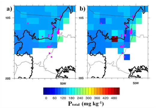
Figure 1.Location and geographical distribution on the regional dataset Ptotal (Quesada et al., 2010) showing the areas of phosphorus sample collection of P-Mehlich-1 in Mato Grosso state. The pink dots are locations of sampling and the thick black line is the geographical limit of the Cerrado biome.

Table 1.Phosphorus content data (P-Mehlich-1) and clay percentage for each sample collected in the Amazon-Cerrado transition region.

Location

Physiognomy Phosphorus Clay

Latitude Longitude n mg kg-1 _%

-15.55 -50.10 1 Cerrado rupestrea _0.89 _30.6

-15.54 -50.10 2 Cerrado típicob _0.20 _34.7

-14.17 -51.76 3 Cerrado raloc _2.28 _21.1

-14.17 -51.77 4 Cerrado raloc 1.30 30.0

-14.15 -51.76 5 Cerrado típicob 2.93 40.5

-14.16 -51.77 6 Cerrado típicob 1.11 35.4

-14.71 -52.35 7 Cerrado típicob 3.00 35.8

-14.71 -52.35 8 Cerrado típicob 0.84 48.2

-14.71 -52.35 9 Cerrado típicob _0.42 _49.3

-14.82 -52.17 10 Semi deciduous Forest 3.18 21.5

-14.71 -52.35 11 Cerrado típicob 0.34 17.3

-14.71 -52.35 12 Cerrado típicob 0.13 17.7

-14.70 -52.35 13 Cerradãod _0.26 _21.0

-14.70 -52.35 14 Cerradãod _0.10 _24.4

-14.69 -52.35 15 Cerradãod _5.46 _21.0

-14.69 -52.35 16 Cerradãod 3.80 33.5

-14.69 -52.35 17 Cerradãod 1.90 40.5

(30)

Table 1. (Continued.)

Location

Latitude Longitude n mg kg-1 _%

-14.69 -52.35 19 Cerradãod 0.30 45.2

-14.72 -52.36 20 Gallery Forest 0.87 15.0

-14.72 -52.36 21 Gallery Forest 6.94 10.5

-14.72 -52.36 22 Flooded Gallery Forest 1.71 11.7 -13.10 -53.39 23 Flooded Riparian Forest 26.0 43.0 -13.10 -53.39 24 Flooded Riparian Forest 18.0 49.0

-13.00 -50.25 25 Cerrado rupestrea 2.44 4.44

-12.38 -50.93 26 Campo de Murundusg 2.30 39.3

-12.36 -50.93 27 Campo de Murundus g 3.30 29.5

-12.04 -50.73 29 Campo de Murundus g _0.70 _38.5

-12.38 -50.93 36 open flooded field 1.60 32.5

-12.83 -52.35 46 Seasonal Evergreen Forest Ptotal= 141 49.0

-12.81 -51.85 47 Seasonal Evergreen Forest Ptotal= 117 16.0

-11.18 -50.23 48 Cerrado densoh _2.71 _3.96

-11.18 -50.23 49 Cerradãod _1.66 _4.16

-11.17 -50.23 50 Cerrado típicob 1.45 3.56

(31)

Location

Latitude Longitude n mg kg-1 _%

-9.79 -50.43 54 Semi deciduous Forest 2.04 18.4

a_{Cerrado rupestre: a tree-shrub vegetation that grows in areas of accentuated topography with many}

rock outcrops and shallow soils, where individual trees establish themselves in clefts in the rocks so that their densities will vary as a function of the specific conditions of each site (Ribeiro and Walter, 2008).

b_{Cerrado típico: a vegetation of trees and shrubs fairly regular and usually not exceeding 4 meters}

(Ribeiro and Walter, 2008).

c_{Cerrado ralo: a vegetation that is more open than Cerrado típico; the trees not exceeding 2 to 3 meters}

in height, covering from 5 to 20% of the soil (Ribeiro and Walter, 2008).

d_{Cerradão: a dense and tall woodland formation (Ribeiro and Walter, 2008).}

g_{Campo de Murundus: a typical landscape of Central Brazil characterized by countless rounded earth} mounds (the ‘murundus’), which are covered by woody ‘Cerrado’ vegetation and are found scattered over a grass-covered surface (the ‘campo’) (Ribeiro and Walter, 2008).

h_{Cerrado denso: this vegetation is more dense than Cerrado típico; the trees exceeding 2 to 3 meters in}

height, and covered with a woody cover ranging from 10 to 60% (Ribeiro and Walter, 2008).

1.2.3 Estimating Ptotal from P-Mehlich-1

The data for the phosphorus content in soil extracted by Mehlich-1 (P-Mehlich-1) was used to estimate the total phosphorus content in the soil (Ptotal). For this, it was first necessary to establish a relationship between P-Mehlich-1 and Ptotal.

(32)

Ptotal and residual. The location, name of the experimental sites, value of Ptotal, PResin and clay percent used to establish the relationship between P-Mehlich-1 and Ptotal are shown in Table A1 (Appendix Table A1).

Based on the Freire (2001) equation, the amount of phosphorus remaining in the soil, i.e., the existing amount of P in the soil (Prem) was estimated for each site, based on their clay content:

Pe = . − . C + . C² R² = 0.747 (1)

where Prem is expressed in mg L-1 and C is the clay content in %. Prem is the P concentration that remains in solution after shaking soil with 0.01 mol L-1 CaCl2 containing 60 mg L-1 P (Alves and Lavorenti, 2006).

After obtaining of the remaining values (Prem), it was necessary to estimate the phosphorus maximum adsorption capacity (CMAP) of each soil, in order to calculate how much phosphorus each soil is capable of adsorbing.

Based on significative data from several studies (Bognola, 1995; Campello et al., 1994; Fabres, 1986; Gonçalves, 1988; Ker, 1995; Moreira, 1988; Muniz, 1983; Novelino, 1999; Paula, 1993), Neves (2000) proposed Equation (2) to calculate CMAP from Prem:

C�AP = . − . log Pe R² = 0.751 (2)

where CMAP is expressed in mg kg-1 and Prem in mg L-1.

(33)

samples data from the work of Bahia-Filho (1982), Muniz (1983), Gonçalves (1988) and Novelino (1999);

P_{−M l} ₋₁

PA = . C�AP

− . _R2 _{= 0.734, (p<0.001)} ₍₃₎

where PAdc is the added dose of P in soil expressed in mg kg-1.

Finally, knowing P-Mehlich-1/PAdc, Presin/P-Mehlich-1 was estimated using the Equation (4) established by Neves (2000) with r=0.899, n=26.

P n

P−M l −1 = .

P−M l −1

PA

.6

R2 _{= 0.808, (p<0.001) (4)}

where Presin is expressed in mg kg-1_.

With the Presin values and the ratio estimated by Equation (4), P-Mehlich-1 values for all stations in Quesada et al. (2010) were estimated (P_m1_est, expressed in mg kg-1). Table 2 shows the estimates obtained by Equations (1), (2), (3) and (4) for the 26 sites in the Amazon.

Obtaining P_m1_est values for locations where data for clay content and Ptotal (mg kg-1) were available, enabled the development of a linear regression model (Equation 5) that estimates Ptotal from P_m1_est (mg kg-1) and C (%) with r = 0.639.

Po a = . + . (P_ _e C) R2 = 0.408, (p<0.001) (5)

(34)

and Discussion) and were incorporated to the regional dataset of Quesada et al. (2010), described in section 1.2.4.

Table 2. Estimates made for obtaining P-Mehlich-1 values for the stations used in this study.

Observation data Estimated data

Quesada et al. (2010)

Presin CMAP �−� � −�

��

� �

�−� � −� P_m1_est

Plot Presin Clay

ID mg kg-1 _% _{mg L}-1_{mg kg}-1 _{mg kg}-1 _{mg kg}-1 _{mg kg}-1

'RIO-12' 3.42 9.50 43.7 404.2 0.27 1.23 2.79

'ELD-12' 5.34 20.1 35.1 486.9 0.21 1.40 3.80

'SCR-01' 2.36 6.88 46.0 384.9 0.28 1.18 1.99

'TIP-05' 9.01 37.3 23.4 637.6 0.15 1.71 5.27

'JRI-01' 1.30 80.7 7.15 1081 0.08 2.51 0.52

'JAS-02' 8.79 29.1 28.6 563.1 0.18 1.56 5.64

'CAX-01' 5.17 41.8 20.9 680.6 0.14 1.79 2.88

'MBO-01' 3.14 11.5 42.0 419.1 0.26 1.26 2.49

'BNT-04' 4.82 57.7 13.4 845.2 0.11 2.10 2.30

'TAP-04' 4.50 89.3 6.18 1136 0.08 2.60 1.73

'ALP-12' 7.37 14.0 40.0 437.9 0.24 1.30 5.67

'SUC-02' 4.06 37.2 23.5 636.7 0.15 1.71 2.38

'AGP-01' 2.99 42.6 20.4 688.8 0.14 1.81 1.66

'ZAR-03' 4.81 31.1 27.3 580.7 0.17 1.60 3.01

'TAP-123' 1.65 66.1 10.5 936.4 0.10 2.26 0.73

'ZAR-04' 7.48 18.3 36.5 471.8 0.22 1.37 5.45

'JUR-01' 10.6 36.6 23.8 631.2 0.16 1.70 6.22

'RST-01' 8.29 25.4 31.2 530.8 0.19 1.49 5.55

'ALF-01' 3.51 11.4 42.1 418.7 0.26 1.26 2.79

'DOI-01' 7.18 19.1 35.9 478.5 0.22 1.39 5.18

'SIN-01' 2.58 9.8 43.5 406.4 0.27 1.23 2.10

'TAM-01' 5.85 37.8 23.2 641.9 0.15 1.72 3.41

'CUZ-03' 11.5 42.5 20.5 687.4 0.14 1.80 6.35

'CRP-01' 21.8 18.1 36.7 470.1 0.22 1.37 15.9

'HCC-21' 7.34 25.6 31.0 532.4 0.19 1.50 4.90

1.2.4 Development and description of the phosphorus regional dataset (PR)

(35)

samples, the average for the Ptotal values (Table 4) was calculated inside each 1° × 1° pixel and the new values added are shown in Figure 2b.

Figure 2. Ptotal regional dataset in mg kg-1 (Quesada et al., 2010) (a), PR with new estimated Ptotal data (b), In both datasets the limit of the Cerrado biome is defined by the thick black line. The sites that provided additional phosphorus data are represented by pink dots.

1.2.5 Description of the global phosphorus dataset (PG)

(36)

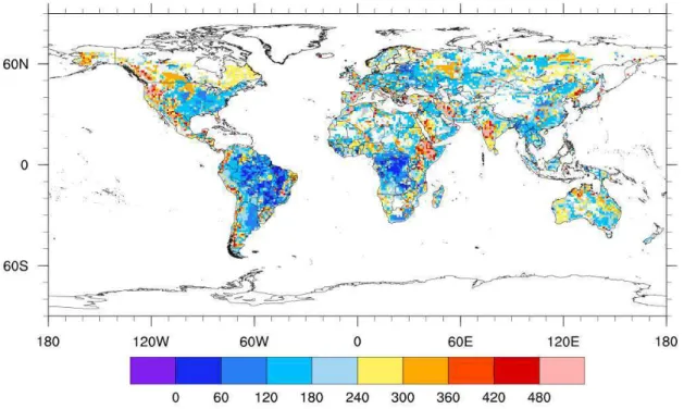
each soil type based on analysis of Hedley fractionation (Yang and Post, 2011) which are part of a worldwide collection of soil profile data.

Figure 3.Map of total phosphorus (mg kg-1_{) in the soil (Yang et al., 2013).}

The uncertainties and limitations of this database are related to the Hedley fractionation data used. When quantified, these uncertainties are 17% for low weathered soils, 65% for intermediate soils and 68% for highly weathered soils (Yang et al., 2013).

1.2.6 Development of Vmax regional and global datasets

The Vmax values in the INLAND model are defined for each plant functional type which, combined in different forms, create the distinct ecosystems represented by the model. Default Vmax values for tropical evergreen trees are defined at 65 µmolCO2 m-2 s-1.

(37)

INLAND model by estimating the maximum capacity of carboxylation by the Rubisco enzyme (Vmax), applying Equation (6) to the regional and global datasets of total phosphorus (PR and PG).

V ax = . Po a + 30.037 (6)

(38)

1.3 RESULTS

1.3.1 Estimates of total phosphorus

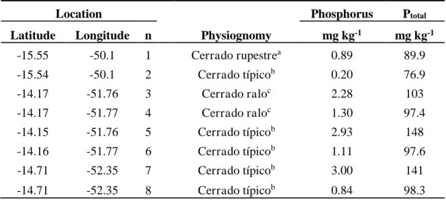
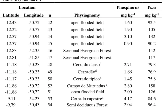
Table 3 shows the total P values estimated for 54 samples of P-Mehlich-1 in Mato Grosso state. These samples were spatialized to a grid of 1° × 1° resolution and resulted in 12 new pixels. Due to the large size of the grid (approximately 111 km), different physiognomies were grouped into a single pixel. For each pixel, the average of Ptotal values was considered regardless of the type of vegetation.

The average values per physiognomy were higher for the Riparian Forest with Ptotal = 11.46 mg kg-1 (n=2) followed by Campo de Murundus with Ptotal = 132.8 mg kg-1 (n=11), Semi deciduous Forest with Ptotal = 106.3 mg kg-1 (n=2), Cerradão with Ptotal = 103.0 mg kg-1 (n=8), open flooded field with Ptotal = 100.8 mg kg-1 (n=11), Cerrado ralo with Ptotal = 100.2 mg kg-1 (n=2), Gallery Forest with Ptotal = 99.8 mg kg-1 (n=2), Cerrado típico with Ptotal = 97.1 mg kg-1_{(n=8), Flooded Gallery Forest with} Ptotal = 85.2 mg kg-1 (n=1), Cerrado rupestre with Ptotal = 84.62 mg kg-1 (n=3), and Cerrado denso with Ptotal = 79.32 mg kg-1_(n=1).

Table 3. Ptotal estimates for the 54 soil samples P-Mehlich-1 in the Mato-Grosso.

Location

Physiognomy

Phosphorus Ptotal

Latitude Longitude n mg kg-1 _{mg kg}-1

-15.54 -50.1 2 Cerrado típicob 0.20 76.9

-14.17 -51.76 3 Cerrado raloc _2.28 ₁₀₃

-14.17 -51.77 4 Cerrado raloc _1.30 _97.4

-14.15 -51.76 5 Cerrado típicob _2.93 ₁₄₈

-14.16 -51.77 6 Cerrado típicob 1.11 97.6

-14.71 -52.35 7 Cerrado típicob 3.00 141

(39)

Location

Physiognomy

Latitude Longitude n mg kg-1 _{mg kg}-1

-14.71 -52.35 9 Cerrado típicob 0.42 85.7

-14.82 -52.17 10 Semi deciduous Forest 3.18 116

-14.71 -52.35 11 Cerrado típicob 0.34 76.2

-14.71 -52.35 12 Cerrado típicob _0.13 _73.9

-14.7 -52.35 13 Cerradãod _0.26 _76.0

-14.7 -52.35 14 Cerradãod 0.10 74.0

-14.69 -52.35 15 Cerradãod 5.46 146

-14.69 -52.35 16 Cerradãod 3.80 154

-14.69 -52.35 17 Cerradãod 1.90 122

-14.69 -52.35 18 Cerradãod 0.80 95.0

-14.69 -52.35 19 Cerradãod _0.30 _81.1

-14.72 -52.36 20 Gallery Forest 0.87 80.1

-14.72 -52.36 21 Gallery Forest 6.94 119

-14.72 -52.36 22 Flooded Gallery Forest 1.71 85.2 -13.1 -53.39 23 Flooded Riparian Forest 26.0 787 -13.1 -53.39 24 Flooded Riparian Forest 18.0 636

-13 -50.25 25 Cerrado rupestrea 2.44 79.4

-12.38 -50.93 26 Campo de Murundusg 2.30 130

-12.36 -50.93 27 Campo de Murundus g 3.30 135

-12.57 -50.91 30 Campo de Murundus g _1.70 ₁₁₅

-12.62 -50.82 31 Campo de Murundus g _2.40 ₁₁₂

-12.38 -50.93 36 open flooded field 1.60 106

(40)

Location

Physiognomy

Latitude Longitude n mg kg-1 _{mg kg}-1

-12.83 -52.35 46 Seasonal Evergreen Forest 142 -12.81 -51.85 47 Seasonal Evergreen Forest 117

-11.18 -50.23 48 Cerrado densoh 2.71 79.3

-11.18 -50.23 49 Cerradãod 1.66 76.9

-11.17 -50.23 50 Cerrado típicob 1.45 75.8

-11,86 -50,72 51 open flooded field 2.00 126

-9.11 -54.23 53 Cerrado rupestrea _4.17 _84.6

-9,79 -50,43 ₅₄ Semi deciduous Forest 2.04 96.4

a_{Cerrado rupestre: a tree-shrub vegetation that grows in areas of accentuated topography with many}

rock outcrops and shallow soils, where individual trees establish themselves in clefts in the rocks so that their densities will vary as a function of the specific conditions of each site (Ribeiro and Walter, 2008).

b_{Cerrado típico: a vegetation of trees and shrubs fairly regular and usually not exceeding 4 meters}

(Ribeiro and Walter, 2008).

c_{Cerrado ralo: a vegetation is more open than Cerrado típico; the trees not exceeding 2 to 3 meters in}

height, covering from 5 to 20% of the soil (Ribeiro and Walter, 2008).

d_{Cerradão: a dense and tall woodland formation (Ribeiro and Walter, 2008).}

g_{Campo de Murundus: are a typical landscape of Central Brazil characterized by countless rounded}

earth mounds (the ‘murundus’), which are covered by woody ‘Cerrado’ vegetation and are found scattered over a grass-covered surface (the ‘campo’) (Ribeiro and Walter, 2008).

h_{Cerrado denso: this vegetation is more dense than Cerrado típico; the trees exceeding 2 to 3 meters in}

height, and covered with a woody cover ranging from 10 to 60% (Ribeiro and Walter, 2008).

1.3.2 Main differences between phosphorus datasets used in this study

(41)

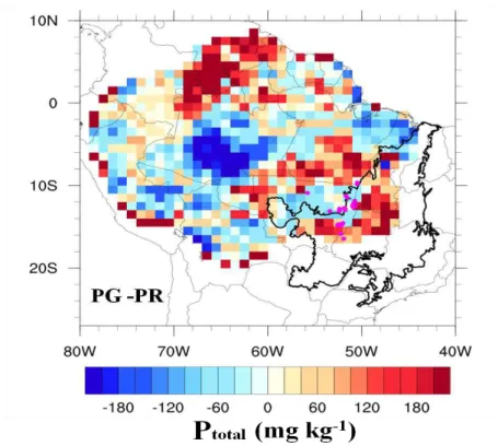
Figure 4. Difference between the global Ptotal maps and regional Ptotal map (PG-PR) in mg kg-1. The Cerrado biome is delimited by the thick black line.

The differences between the absolute values of total phosphorus at a spatial resolution of 1° × 1° varied in the range of ±180 mg kg-1_{, with an average of} 24.19 mg kg-1.

1.3.3 Vmax maps used in this study

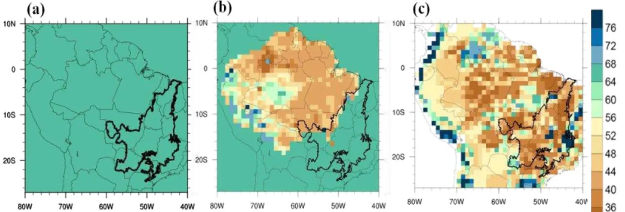
Equation 6 was applied to the regional map of Ptotal (Section 1.2.6) to obtain the regional Vmax map (PR), and to the global Ptotal map (Section 1.2.5) to generate the global Vmax map (PG). Figure 5 shows Vmax calculated from the P datasets. In Figure 5a, all pixels received the same value for Vmax (65 μmolCO2 m-2 s-1), corresponding to the default settings of INLAND. In Figures 5b and 5c it is possible to observe that the Vmax data followed the spatial gradient of the total P content in soil, with values varying

(42)

Figure 5. Default Vmax value of INLAND ‒ PC (a), Regional Vmax dataset ‒ PR (b), Global Vmax dataset ‒ PG (c), all in µmolCO2 m-2 s-1.

The estimated values of Ptotal in the Amazon-Cerrado border were used to expand the regional P map used by Castanho et al. (2013) and thus generate the Vmax map shown in Figure 5b. These new values are described in Table 4 and range from 37.9 to 102.1 μmolCO2 m-2 s-1.

Table 4. Vmax values and Ptotal values for samples in the Amazon-Cerrado transition region.

Samples Average Ptotal Vmax

n=54 Pixel mg kg-1 _{µmolCO2 m}-2_s-1

2 1 83.38 38.48

4 2 111.6 41.34

16 3 101.5 40.32

2 4 711.5 102.1

1 5 79.39 38.08

20 6 114.3 41.62

1 7 141.5 44.38

1 8 117.0 41.89

3 9 77.32 37.87

2 10 141.7 44.39

1 11 84.61 38.61

(43)

1.4 CONCLUSIONS

The recent availability of phosphorus data in the Amazon made possible the development of a model able to estimate Ptotal throught P-Mehlich-1, thus extending the regional soil map in the Amazon-Cerrado transition. This methodology allows new estimates of Ptotal to be obtained from P-Mehlich-1 data collected in the field, using a robust model with 99% confidence in the estimates.

Although a model was developed to estimate Ptotal in the soil, it is recommended that future works interested in evaluating the P content in the plants should not collect only the labile P, but use the Hedley fractionation method, which informs all forms of P for the given soil sample.

(44)

CHAPTER 2 – Effects of climate, fire and phosphorus in the Amazon-Cerrado border simulated with INLAND model ‒ Numeric experiment development

2.1 INTRODUCTION

The transition between the Amazon and Cerrado in Brazil has the largest area of contact between forest and savanna in the tropical regions and these biomes differ fundamentally in their structural characteristics and species composition (Torello-Raventos et al., 2013). In this transition, climate seasonality – especially precipitation – and fire disturbances have an important role in the balance of the vegetation due to influences of the ecological and biogeochemical processes of vegetation directly affecting the carbon fluxes (for example, the Gross Primary Production – GPP, Net Primary Production – NPP and respiration) that, over time, may lead to changes in composition and structure of vegetation (Alves et al., 1997). Tree species associated with forest or savanna vegetation differ in numerous physiological characteristics, such as fire survivorship (Hoffmann et al., 2009; Ratnam et al., 2011), as well as in their wood and foliar characteristics (Gotsch et al., 2010), sometimes related with soil fertility (Ferreira-Ribeiro and Tabarelli, 2002; Miranda et al., 2003; Quesada et al., 2012). Generally, we have an incomplete knowledge on how the trees of these vegetation types differ in photosynthesis characteristics, especially in terms of response to nutrient availability.

(45)

the quantification of phosphorus is poor, since it was believed that, in contrast to tropical forests, photosynthetic capacity in the savannas would be more likely to be limited by N than by P (Lloyd et al., 2009).

However, works from West Africa showed that, depending on the relative concentrations of P and N in the leaves, both Rubisco activity and electron transport activity of African savanna and forest trees can potentially be limited by either N or P (Domingues et al., 2010), so there is no consensus about how the vegetation is limited by these nutrients and how this limitation associated with factors such as climate and fire could act on the areas of transition in a scenario of future climate change. Numerous efforts through dynamic vegetation models (DGVMs) have been conducted on Amazonia forests with the aim of understanding dynamics through the analysis of long-term field observations of tree growth and mortality patterns as they relate to climatic and edaphic variations across the basin (Castanho et al., 2013; Phillips et al., 2004; Quesada et al., 2012).

(46)

(47)

2.2 MATERIALS AND METHODS

2.2.1 Description of the INLAND Surface Model

The INLAND model is the main and the first land-surface component of the Brazilian Earth System Model (BESM). INLAND is based on the IBIS model (Foley et al., 1996) which considers changes in the composition and structure of vegetation in response to the environment and incorporates important aspects of biosphere-atmosphere interactions in South America. The model simulates the exchanges of energy, water, carbon and momentum between soil-vegetation-atmosphere. These processes are organized in a hierarchical framework and operate at different time steps, ranging from 60 minutes to 1 year, coupling ecological, biophysical and physiological processes (Kucharik et al., 2000). The vegetation is represented by two layers, upper and lower canopy, and 12 plant functional types (PFTs): tropical evergreen trees, tropical deciduous trees, temperate evergreen trees (broadleaf), temperate evergreen trees (conifers), temperate deciduous trees (broadleaf), boreal coniferous evergreen trees, boreal deciduous trees (broadleaf), boreal deciduous trees (coniferous), perennial shrubs, deciduous shrubs, herbaceous C3 and grasses C4. The combination of the 12 PFTs creates the distinct ecosystems represented by the model: tropical evergreen forest, tropical deciduous forest, temperate evergreen broadleaf forest, temperate evergreen conifer forest, temperate deciduous forest, boreal evergreen forest, boreal deciduous forest, mixed forest, savanna, grassland, dense shrubland, open shrubland, tundra, desert and polar desert or ice.

(48)

concentration, and the Rubisco enzyme capacity for photosynthesis (Vmax). The maintenance respiration is a function only of Vmax. The yearly dynamic vegetation module computes the following for each PFT: gross and net primary productivity (GPP and NPP), changes in biomass pools, simple mortality disturbance processes and resultant Leaf Area Index (LAI), thus allowing vegetation type and cover to change through time. GPP and NPP are calculated at the end of each year as:

GPP = ∫ �� (7)

�PP = − � ∫ ��, � − �� ,�− �� ,�− ��,� �� (8)

where η (0.33) is the fraction of carbon lost in the construction of net plant material because of growth respiration (Amthor, 1984). The partitioning of the NPP for each plant functional type resolves carbon in three biomass pools: leaves, stems and fine roots. The leaf area index (LAI) of each PFT is obtained by simply dividing leaf carbon by specific leaf area, which in INLAND is considered fixed (one value) for each PFT.

The soil physical properties in INLAND used a multilayer formulation of soil (eight soil layers) to simulate the diurnal and seasonal variations of heat and moisture. Each layer is described in terms of soil temperature, volumetric water content and ice content (Foley et al., 1996; Thompson and Pollard, 1995). Furthermore, all of these processes are influenced by these soil texture and amount of organic matter within the soil profile.

(49)

The soil chemical properties are represented by the carbon cycle (C), nitrogen (N) and phosphorus (P), the latter being recently implemented by Castanho et al. (2013). The carbon cycle is simulated through vegetation, litter and soil organic matter, where the biogeochemical module is similar to the CENTURY model (Parton et al., 1993; Verberne et al., 1990). The amount of C existing in the first meter of soil is divided into different compartments characterized according to their time residence, which can vary in an interval of a few hours for microbial biomass and organic material to several years for lignin. For the nitrogen, the model considers only the soil N transformations and carbon decomposition, not influencing the productivity of vegetation, ie., there is a fixed C:N ratio. Phosphorus is used only to limit the net primary productivity. The total phosphorus available in the soil is used to estimate the maximum capacity of carboxylation by the enzyme Rubisco (Vmax) through a linear relationship, Equation 6.

(50)

INLAND also contains two fire modules. The first module is a simple fixed-value disturbance, which does not depend on the environmental conditions. The second module is based on the fire module of the Canadian model of fire CTEM (Arora and Boer, 2005). In this module, all three aspects of the fire triangle ‒ the availability of fuel to burn, the flammability of vegetation depending on environmental conditions, and the presence of an ignition source ‒ are taken into account. Here, CTEM uses an arbitrary anthropogenic fire probability which is summed to the natural ignition probability.

2.2.2 Model Configuration and Experiment Design

The model was forced with a prescribed climate based on the Climate Research Unit (CRU) databases of the University of East Anglia (New et al., 1999). Two boundary conditions were used; the first is referred to as the monthly climatological average (CA), commonly used by the scientific community to represent the average climate of a 30 year period of the last century (1961-1990). The second boundary condition is the historical dataset, used to represent the actual climate variability for the period 1948-2008 (CV), a continuous record of 61 years. The dataset has a 1-degree spatial resolution and a monthly time resolution.

Soil texture data is based on the IGBP-DIS global soil (Global Soil Data Task 2000) (Hansen and Reed, 2000), and the Quesada et al. (2010) dataset. All of the simulations started with the potential vegetation defined by the Center for Sustainability and the Global Environment (SAGE)(Ramankutty and Foley, 1999), with soil carbon and litter pools set to zero.

(51)

380 ppm and no fire effects (fire module off), for a period of 428 years (equivalent to the period 1581-2008). In the control run (PC) the Vmax data used to calculate productivity were the default global value used by the dynamic vegetation module of the INLAND (65 μmolCO2 m-2_s-1_{) for the plant functional types: tropical evergreen} trees and tropical deciduous trees. Simulations with different combinations between the climate scenarios (CA and CV), different nutritional limitation scenarios provided by Vmax maps (PR and PG), fire effects (F) on or off, and the effects of CO2 fixed (380 ppm) or variable CO2 (270 ppm to 385 ppm) were also performed. A summary of the simulations are presented in Tables 5 and 6.

Table 5. Simulations with different combinations of the factors evaluated by INLAND model considering the climate scenario CA, climatological average (1961-1990).

CO2 Fire (F)

Vmax

PC PR PG

Fixed Off CA+PC CA+PR CA+PG

Fixed On CA+PC+F CA+PR+F CA+PG+F

Variable Off CA+PC+CO2 CA+PR+CO2 CA+PG+CO2

Variable On CA+PC+F+CO2 CA+PR+F+CO2 CA+PG+F+CO2

Table 6. Simulations with different combinations of the factors evaluated by INLAND model considering the climate scenario CV, 1948-2008 monthly data.

CO2 Fire (F)

Vmax

PC PR PG

Fixed Off CV+PC CV+PR CV+PG

Fixed On CV+PC+F CV+PR+F CV+PG+F

Variable Off CV+PC+CO2 CV+PR+CO2 CV+PG+CO2

Variable On CV+PC+F+CO2 CV+PR+F+CO2 CV+PG+F+CO2

(52)

in the NPP, biomass and LAI, and their consequent effect on the position of the Amazon-Cerrado border.

2.2.3 Analysis of the Model Sensitivity

Analyses were performed for the individual effects of climate, phosphorus, fire and CO2 on the explanatory variables: Net Primary Production (NPP), biomass, and leaf area index of the upper and lower canopy (LAIupper, LAIlower).

Analysis of the isolated effect of climate variability was performed using a combination of CV+PC and CA+PC, so that the subtraction between the simulations presents the effect of climate variability isolated: (CV+PC) - (CA+PC) = (CV-CA)|PC; in other words, this is the effect of climate variability for default Vmax (PC).

The same logic was applied to isolate factors such as fire and phosphorus in different climate scenarios, e.g. the isolated effect of fire with an average climate scenario without influence of nutritional limitation is calculated by the difference between CA+PC+F and CA+PC, so that (CA+PC+F) - (CA+PC) = F|CA PC. The isolated effect of fire with a climate variability scenario without influence of nutritional limitation is calculated by the difference between CV+PC+F and CV+PC, so that (CV+PC+F) - (CV+PC) = F|CV PC.

(53)

Table 7. Individual and combined effects for each simulation.

Combined Effects

A B C D E

Climate Phosphorus (P) Fire (F) CO2 CO2+F

1 (CV+PC)-(CA+PC) (CA+PR)-(CA+PC) (CA+PC+F)-(CA+PC) (CA+CO2+PC)-(CA+PC) (CA+PC+F+CO2)-(CA+PC) 2 (CV+PR)-(CA+PR) (CV+PR)-(CV+PC) (CV+PC+F)-(CV+PC) (CV+CO2+PC)-(CV+PC) (CV+PC+F+CO2)-(CV+PC) 3 (CV+PG)-(CA+PG) (CA+PG)-(CA+PC) (CA+PR+F)-(CA+PR) (CA+CO2+PR)-(CA+PR) (CA+PR+F+CO2)-(CA+PR)

4 (CV+PG)-(CV+PC) (CV+PR+F)-(CV+PR) (CV+CO2+PR)-(CV+PR) (CV+PR+F+CO2)-(CV+PR)

5 (CA+PG+F)-(CA+PG) (CA+CO2+PG)-(CA+PG) (CA+PG+F+CO2)-(CA+PG)

6 (CV+PG+F)-(CV+PG) (CV+CO2+PG)-(CV+PG) (CV+PG+F+CO2)-(CV+PG)

Effects

A B C D E

4 P (G-C)|CV F |CV PR CO2|CV PR CO2+F|CVPR

5 F |CA PG CO2|CA PG CO2+F|CA PG

(54)

2.2.4 Determination of the best model configuration

The performace of each model configuration to determine the Amazonia-Cerrado border was evaluated using two different metrics: The first metric is the correlation between total dry season LAI simulated by the model and the MODIS dry season LAI product in five longitudinal transects along the Amazon-Cerrado border, (described in Section 2.2.5). The second metric is correlation between simulated biomass and biomass data provided by Nogueira et al. (2014). The value of biomass was estimated by matching vegetation classes mapped at a scale of 1:250 000 and 29 biomass means from 41 published studies for vegetation types classified as forest (n=2317 plots) and as either non-forest or contact zones (1830 plots). For more details, see Nogueira et al. (2014).

2.2.5 Development of the MODIS LAI Map

The MODIS product used in this work is the MOD15A2, which is responsible for providing leaf area index data every 8 days, totalizing 46 images per year. When drawing up the MODIS LAI map, nine images per year were used, corresponding to the months of July, August and September, for the period of 2000-2008, amounting to 81 leaf area index images. These images were filtered by annual coverage maps and land use also provided by MODIS through the MOD12Q1 product in order to delete information from areas of non-natural vegetation. The filter was made considering a spatial resolution of 1 km.

(55)

the classes: cropland cover (12), urban and built-up (13), cropland/natural vegetation mosaics (14) and sparsely vegetated barrens (15). Then bi-linear interpolation to one-degree resolution was performed and the average of all images resulted on the average dry season leaf area index MODIS (LAIdry), shown in Figure 7.

Figure 7.Map of the average dry season (July, August and September) leaf area index of MODIS product MOD15A2 from 2000 to 2008 and the five transects used in this study.

2.2.6 Statistical Analyses

(56)

2.3 RESULTS AND DISCUSSION

2.3.1 Comparison of simulations (Isolated Effects)

In this section we present the results of the isolated effects of climate, phosphorus, fire and CO2 in the NPP, biomass and LAIlower and LAIupper canopies.

2.3.1.1 Climate effects

Figure 8 shows the influence of the average climate (CA) and interannual variability (CV) on NPP, biomass, and LAIupper and LAIlower.

For both climate conditions used (CA and CV), the INLAND represents well the Amazon-Cerrado transition (Figure 8a and 8b) with higher NPP values in the forest region and lower values in Cerrado.

NPP estimates from INLAND for the Amazon forest were compared against field data from LBA project and RAINFOR network sites (from KM67, ZF-2, UFAC, AGP, CAX, TAM and ZAR) described in Table 8.

(57)

Table 8. NPP estimates from the INLAND and the relative errors for the KM67, ZF-2, UFAC, CAX, TAM, ZAR and AGP sites.

Site Period Observed NPP

Average observed

NPP

NPP INLAND

Error %

Error % CA+PC CV+PC CA+PC CV+PC

KM67 2001 1.23

1.14 1.24 0.94 9 -24

2004 1.06 -11

ZF-2 2001 1.06

1.21 1.22 1.11 1 4

2002 1.36 -18

UFAC 2001 1.34

1.32 1.26 1.16 -5 -14

2002 1.30 -11

CAX 2004-2006 1.40 1.40 1.22 1.10 -13 -21

TAM 2005 1.53 1.53 1.42 1.27 -7 -17

ZAR 2004-2006 0.93 0.93 1.23 1.13 32 22

(58)

Figure 8. Climate variability effect on NPP, biomass, LAIupper and LAIlower. The hatched areas indicate that the variables are statistically different compared to the control simulation at the level of 95% according to the t- test and the thick black line is the geographical limit of the Cerrado biome.

(59)

from 1.2 to 0.8 kg-C m-2_yr-1 _{with a northwest-southeast gradient in Amazonia, and in} Cerrado range between 0.2 and 0.8 kg-C m-2 yr-1 (Figure 8). In percentage terms, NPP decreases 11% in the Amazon and 15% in the Cerrado, when the climate variability was considered.

The decrease in NPP is a consequence of the higher frequency of extreme precipitation, temperature and radiation associated with interanual climate variability, causing differences in the photosynthesis and annual carbon balance. In the Cerrado, the differences between CA and CV were higher because in this biome the seasonal variability of climate affects more intensely the vegetation, exposing the trees to soil water stress, decreasing the NPP more than in the Amazon region, where the seasonality of climate is less pronounced.

The small difference between total NPP values in CA and CV is probably related to the fact that there is offsetting between the LAIupper and LAIlower, which causes the total carbon fluxes to vary little when only the climate varies (Figure 8). This result confirms the findings of Botta and Foley (2002), who found low sensitivity of total LAI and NPP simulated by the IBIS model to interannual climate variability. LAI is an important variable in the INLAND model because it is the main variable used to determine the dominant vegetation type that is assigned to a pixel. The simulated LAI follows the NPP gradient, with values ranging approximately from 5 to 11 m2 m-2 for LAIupper in the Amazon and 0 to 6 m2 m-2 in the Cerrado (Figure 8g and 8h). For LAIlower these values range between 0 and 6 m2_m-2_{in Cerrado and close to zero in} Amazonia (Figure 8j and 8k).

(60)

it can be observed predominance of trees instead of grasses, except for the western region of the state of Mato Grosso, where higher LAIlower values can be observed (Figures 8j and 8k). In the central region of the Cerrado, a small area (along 45°W) with relatively high LAIupper values (Figures 8g and 8h) and low values LAIlower (Figures 8j and 8k) are found, featuring a forest in both climate scenarios.

The LAI simulated values are qualitatively representative, but they are probably overestimated. In the Amazon, LAI values generally vary from 4 to 8 m2_m-2_(Carswell et al., 2002; McWilliam et al., 1993) and they are, in general, larger than the LAI observed in Cerrado. According to Miranda et al. (1997) and Hoffman et al. (2005), observed LAI in Cerrado range from below 1 to 2.5 m2 m-2. In the Amazon region, the CV LAIupper decreased 11.9%, and 12.5% in the Cerrado with respect to the CA simulation, while for the LAIlower, it increased 37% in the Amazon and 548% in Cerrado. The increase of 548% of LAIlower results from areas dominated by very low LAIlower values in CA (ie. areas between 10° S and -8° S in Cerrado domain, Figure 8k) and increased in CV to 6 - 7 m2 m-2.

(61)

the whole Amazon, when CV was used a reduction os arboreal biomass of 10.7% was found, while in the Cerrado, there was an increase of 5%.

2.3.1.2 Phosphorus effect

The analysis of the phosphorus effect under variable climate indicates that the carbon assimilation was strongly limited by the phosphorus availability in the Amazon and the reduction in the NPP was significant for most of the Amazon area for both PR and PG datasets with respect to the PC control simulation (Figures 9 and 10). The decrease in NPP was approximately 0.2 and 0.4 kg-C m-2 yr-1 for PR and PG respectively, when compared to PC, except a few pixels in northeastern Amazonia where NPP decreased by more than 1 kg-C m-2_yr-1 _{for PG simulations.}

In Cerrado, when PR was considered, the decreases in the NPP range from 0.1 to 0.2 kg-C m-2 yr-1 and were statistically different only in the new pixels added to the phosphorus regional dataset, as expected (Figure 9a).

In contrast, we found a small decrease in NPP for most of the Cerrado area when we considered PG. Although the decrease is not statistically significant, except for one pixel close to 52° W, it influences the decline on biomass in Cerrado (Figure 10b).

(62)

the INLAND model in this biome is dominated by grass, which is not influenced by P in the model.

The spatial variability of LAIupper (Figures 9c and Figure 10c) and biomass (Figures 9b and Figure 10b) for PR and PG reflect the spatial patterns of NPP along the Amazon-Cerrado transition.

The biomass decreased in the northwest of Amazonia and in the south (between Amazonas, Pará and northern of Mato Grosso states) from 2 to 5 kg-C m-2 (Figure 9b) when PR was considered. The biomass gradient shows that the regional nutritional limitation is strongly influenced the boundary between Amazonia-Cerrado, following the trend of a more weathered area poor in soil P in the southeastern Amazon (Quesada et al., 2009).

On the other hand, when PG was used, a higher decrease in biomass was shown in Central Amazonia, in the northeast of Pará and in the northeast of Mato Grosso (Figure 10b), which agrees with the study of Mendes et al. (2013), which demonstrated that there is a close relationship between carbon assimilation and leaf phosphorus, in this region. Although the datasets have presented a different spatial gradient, both revealed that phosphorus limitation is higher in Amazonia than in the Cerrado.

(63)

Figure 9.Regional Phosphorus effect (PR) on NPP (a); biomass (b); LAIupper (c); and LAIlower (d). The hatched areas indicate that the variables are significantly different compared to the control simulation at the level of 95% according to the t- test and the thick black line is the geographical limit of the Cerrado biome.

(64)

Figure 10. Global Phosphorus effect (PG) on NPP (a); biomass (b); LAIupper (c); and LAIlower (d). The hatched areas indicate that the variables are significantly different compared to the control simulation at the level of 95% according to the t- test and the thick black line is the geographical limit of the Cerrado biome.

2.3.1.3 Fire Effect

Overall, fire has an effect decreasing Cerrado biomass, decreasing upper canopy LAI and allowing the increase of the lower canopy LAI (Figure 11). Small parts of the dry forest also suffered the same effect, mainly in Rondonia, Bolivia and southern Peru.

(65)

increases in LAIlower between 1 and over 5 m2_m-2_{. In Mato Grosso state, where} transition is longest the increase of LAIlower was above 4 m2 m-2 which indicates high fire activity.

In the Amazon, the small decrease of arboreal biomass in simulations reinforce the idea that the Amazon rainforest is naturally impervious to fire, contrary to the tropical savannas, which are naturally influenced by this disturbance (Lehmann et al., 2011; Murphy and Bowman, 2012). This influence of fire in tropical savannas has a great ecological importance and has been, for example, associated with the expansion of savannas in drier climate conditions as a major contributing factor (Couto-Santos et al., 2014; Silvério et al., 2013). Our results show that the fire effect in the Cerrado domain along the transition implies significant increases in LAIlower, that represents shrubs and herbaceous vegetation (Figure 11g, Figure 11h, Figure 11i) and decreases significantly in LAIupper (Figure 11d, Figure 11e, Figure 11f), that represents trees, thus influencing the dynamics of upper and lower canopies. Under conditions of a future climate change scenario, this competition between trees and grasses can lead to a change in vegetation structure, favoring the expansion of grasses (Malhi et al., 2009).

In the Amazon domain along the transition it is evident that, although there was a significant decrease of the biomass (Figure 11a, Figure 11b, Figure 11c) in response to fire, the decrease in leaf area index was not of the same proportions (Figure 11d, Figure 11e, Figure 11f). This may be due to the much smaller time needed to build a leaf (< 1 year), when compared to the typical interval between disturbances in the forest region (several years).

(66)

comparison to the Cerrado domain, and the latter is dominated by the presence of a continuous grassy layer that regains its flammability very quickly after burning. The Amazon is less flammable, generally burns less frequently and with less intensity, which allow this biome to maintain a dense canopy with distinct ecosystem properties (Eldridge et al., 2011). In the transition, the fire effects on LAIupper and LAIlower were inversely related. The decrease in the LAIupper led to an increase in radiation available to the lower canopy, which led to the spread of a shrub and herbaceous component. Therefore, there was a significant increase in LAIlower, ranging up to 5 m2 m-2 in many places in the Cerrado.

(67)

2.3.2 Longitudinal gradient of biomass and leaf area index in the Amazonia-Cerrado transition ‒ Field observations

The five longitudinal transects used in the transition’s analysis showed higher values in the west and lower values in the east for biomass (Nogueira et al., 2014) and dry season MODIS leaf area index (LAIdry) (Figure 12). This gradient agrees with the trends observed by Malhi et al. (2006), who found higher biomass in the central Amazon compared to lower values in the southeast Amazon region. Observed data fields in the transition region are limited, and the existing data are estimates based on small samples, which reduces in part its reliability. On the other hand, remote sensing data such as MODIS are an alternative to large-scale studies because they provide good estimates of LAI, contributing to information on the dynamics and structure of vegetation.

(68)

(2014), and therefore were excluded from the correlation analysis. In the central Amazonia-Cerrado transition, the observed biomass and LAIdry MODIS showed better correlation with higher values (R). The data for all transects were used in the next Section (2.3.3) for comparison with INLAND model simulations.

(69)

2.3.3 Longitudinal gradient of biomass and leaf area index in the Amazonia-Cerrado transition ‒ Comparison between simulations and field observations

The comparison of simulated results considering the different combinations between nutritional limitation (PR and PG), occurrence of fire (F), interannual climate variability (CV) and average climate (CA) against the dry season LAI (MODIS- LAIdry) and biomass data are presented in this Section.

All transects simulated show overestimated LAI (sum of LAIupper and LAIlower) values and underestimation of biomass values (Appendix, Figures A1 and A2). Although the difference between simulated and observed values are not small, the INLAND model was able to adequately represent the longitudinal gradient for all transects, with higher values to the west and lower LAI and biomass values to the east. The correlations between simulated and observed values of LAI and biomass were higher when considering the interannual climate variability scenario (CV) for most transects, with average values of 0.49 for LAI and 0.71 for biomass (Tables 9 and 10). Table 9. Correlation coefficients of dry season LAI simulated by INLAND and remote sensing estimates by MODIS.

T1 T2 T3 T4 T5 Transects

average

CA CV CA CV CA CV CA CV CA CV CA CV