Non-Linear Distance Transformation Algorithm and
its Application in Medical Image Processing in
Healthcare
Yahia S. AL-Halabi, Professor of Computer Science
Computer Science Department, King Hussain Faculty for Computing Sciences Princess Sumaya University for Technology (PSUT)
Amman, Jordan
Abstract—Medical image processing is one of the most demanding domains of the computing sciences. The importance of the domain is in terms of the CPU and the memory requirements that shall be used by the system to compute the result. Moreover, the volume of the data is often very large in terms of the space and primarily requires many processing tools. At the same time, the tools have to be available as the real time applications, in order to be used by the physicians On the other hand; computational complexity is also another significant issue in the processing of the data. Therefore, the development of advanced and optimized algorithms is now sought as the way to improvise the effectiveness of the processing and development capability of the image processing systems. Thus, distance map (DT) has emerged as one of the most influential types of algorithms to enhance the computational capacity of the unit and further produce better results for the actual outcome of the system. The results of the output have been in high favour of the distance map algorithm. Moreover, the output has witnessed an increasing trend in the performance of the system and has been quite prominent in terms of acquiring the resources. The results of the conclusion has concluded the fact that, the application of the distance map algorithms has resulted in the reliable alternative that can be applied in the field to improvise the running norms and further speed up the existing procedures.
Keywords—Distance map; complexity; nonlinear; medical; image processing
I. INTRODUCTION
It is highly mandatory to have developed methods that can be used to maximize the output with having least amount of input to supply. After the through considerations of all the cases, it has been cited that; most of the modern day application makes the use of the computational devices that can are further facilitating the user in the wellbeing of the subjected cause. Thus, the computational robustness and optimum performance is thought of as highly influential point in evaluating the recital of the system [1-3].
Like most of the domains, the computational advancements have slipped their way in the medical industry as well with having the aim to serve the humanity to the maximum of the extent. In addition, various applications in the domains have supplied with ample of benefits with addressing almost every sub routine of the medical industry. Out of them, medical image processing is one of the most
emerging forms of the computational applications that are heavily supplying with befits to the field of the medical sciences. Medical image processing needs continuous enhancements in terms of the techniques and the procedures that are being followed to gain the desired output. Furthermore, the field needs some serious efforts that can be applied to improve the quality of the services in the health care industry. In this regard, scholars and scientists have brought up various techniques that can be used to improvise the entire output of the system [4]. The techniques include; image compression, image interpolation or image registration. Keeping in mind, all of these techniques are destined to be improved to be abreast with growing demands of the emerging industry. However, the ever growing demands of the medical image processing are in development along with the technologies pertaining to mobile and computing technologies.
Growing interest in the health care domain has paved its way for the upbringing of the innovative and robust approaches for medical diagnosis and clinical practices. As per the saying of the scholar “Health is Wealth”; various personnel are coming up with the efforts to use innovative medical procedures and treatment that can be coupled with technologies in computations, to harness advancements in the hardware resources. After the thorough analysis of the medical industry, it has been found that, the field needs advanced and accurate methods for the diagnosis of the disease with maximum accuracy in the clinical practice. Therefore, the emerging needs in the market has posed the proposition of best practices which are clinically proven. However, the field is still at open notches in terms of the advancements and still many efforts are required to be carried out to unveil the hidden knowledge and maximize the operational flow of the medical industry [1-6].
the processing time and further make it worthy to be applied in the field. In this regard, various scholars have come up with exceptional; yet, remarkable algorithms that can be used to reduce the computational complexity of the medical image processing [4-6, 8].
Along with the added advancements in the processing peripherals, the processing algorithms are categorised under the linear and nonlinear process. The complexity is counted as one of the main obstructions that hinders in the successful execution of the program. Therefore, the consideration has led to a sense of need of such algorithms that are easy to implement along with having the least consequences to bear in terms of the operations that are exhibited by the system [7, 9]. Apart from the successful upbringing of the algorithms, the researchers also have to take care of the complexity that is being held by the system. One of the main reasons for the reduction of the complexity is that, the medical image processing is applicable in real time environments; therefore, it should take the least time to respond to a subjected cause along with the proper processing of the result. The system; since working in the real time must be agile enough to resist any kind of lacks in the executional operations of the system. Moreover, a slightest of the lack in the outcome of the system can result in the production of unwanted and vague results that may not be addressing to the actual scenario. Hence, the reduction of the computation complexity along with maximizing the production of the output of the system is set as one of the primary aims of the computational systems. Therefore, the same evaluation phenomenon applies to the evaluation of the medical imaging units [8]. According to a study, it has been found that, health care industry generates huge amount of data. Thus, the scientists have to consider the proposition of the intelligent processing of such data items that can be used to reveal the hidden relationship among the data items that shall be helping in the improvisation of the clinical practices. On the other hand, the exponential growths in the medical image processing can further improve the standards of the health that are provided to the citizens and in turn reduce the death toll of the entire state. In a whole, it can be said that, medical image processing can help to reduce the diagnosis overheads from the identification of the disease and in turn can helpful in providing the procedures that may be in the best of the interest of the human beings [10].
The most common problems of non-linear computational systems have been mentioned and discussed involving results for computational systems. The asymptotic stages of non-linear computational complexities were potetntial by demanding the sequences that converge the given state into its finite period. The non-linear computational complexities can be appeared into four definite problems. These problems are sub-dividied into 2 design problems: design problem and analysis problem. Furthermore, it is important to observe that algorithms can be used for the corresponding analysis problems when exist for design problem [4, 5, 9]. Therefore, analysis problem are considered to be more easier than design problem to solve. However, analysis problems are harder to illustrate undecideable rather than control problems, when heading towards negative complexity-theoritic results.
In order to focus on these problems, it is important to predict that the system is given in regards of a finite-length description of the function. Moreover, the problems are stated into polynomial time whereas there has been no algorithms present for non-linear systems. It is considerable to discuss that these problems are not interesting to be difficult if they are stated at the level of generality. The problem of non-controllability for common non-linear systems entailed the issues of deciding whether the given non-linear equation has a solution or not. The null-controllable function can be stated as zero, if the function given is considered as null-controllable. Therefore, the null-controlability problem for non-linear computational systems is considered to be difficult to decide whether a given non-linear system has a zero. The types of non-linear systems considered are restricted while focusing towards the intrested problems. The types of non-linear can be classified into two main types: systems with component wise non-linearlities and systems with a single non-linearity [13].
Algorithms are inherently ineffiecint for those systmes that are included in a single scalar non-linearlity. In order to look at this system, an arbitraty non-linear scalar function must be fixed that satisifies
����→−∞�(�)≤ ����→+∞�(�), ∀� ∈ � (1)
The problem must be considered after fixing the arbitrary
function in which ��,��∈ �� are given as input and all trajectories of the
system must be determined in order to converge into the origin. The non-linear system would be considered as linear system if this equation is decided in polynomial time. However, the problem can be considered as the NP-hard for any definite non-constant v. an NP-hardness result can be obtained for a very simple class of non-linear systems, if we focus on the particular case where v is the sign function. It has been reported that these types of systems can be arouse when a non-linear system is controlled by using a controller whereas they also illustrate one of the simplest types of non-linear systems [11, 12].
Chaotic dynamics usually points towards the deterministic development with chaotic results. Nonlinearity in a system generally means the measured values of a system’s properties in a later state rely in a complex way on the measured values in the early state. By complex, it meant something other than the proportional to, or some combination of these two differing by a constant. Although by these statements, it does not mean to imply somewhat complicated phenomena cannot be modelled by linear relationships. The non-linear simple mathematical example would be for noticeable for x in the (n+1)th state which rely on the square of the observable x in the nth state is ��+�=���. These relations are termed as mappings and this is a simple and general example of a non-linear map that exist in the nth state to the (n+1) th state [12].
of these sets of equations. Non-linear relations are not adequate for chaos, but few of the nonlinearities are required for chaotic dynamics [11, 12]. Considering the briefly nonlinear mappings, it has been considered more closely systems modelled by different forms of differential equations to write them in a standard first-order form:
�=�(�,�) (2) If the function f is independent of t then the equation is said to be autonomous and if f is not independent then it is non-autonomous. It must have more than one degree of freedom or being non-autonomous for such systems.
The researchers who are working with the non-linear programming techniques claims the word ‘non-linear’ that indicate the real applications needed for non-linear modelling. This is true for the areas where there are always several goals in real applications, stochastic programming where the data is uncertain and so forth. The quadratic maps and non-linear oscillator might not appear to offer rich diversity of chaos [9].
One of the major objectives is to categorize and classify the deterministic systems that exhibit chaotic dynamics. However, the characterization of the nonlinearity is an important ingredient for the chaotic dynamics that marks the beginning of the classification effort.
The dynamics determined by the field of vector ��(�) and it can be highly complicated. The specific fixed points are of special interest and they are readily recognized as just those values of x for which ��(�)= 0. Fixed points may be stable or unstable and so the behaviour of fixed points is significant. Moreover, ��(�) represents the updated value of the function that has been computed after the proper evaluation of the supplied values.
�(�) =�(��) +��(��)(� − ��) +⋯ (3)
where Df (��) is the matrix of function that is evaluated at the fixed point x. it is clearly true that x is a fixed point of the map and it can be characterized by the fixed points and stability of maps in a manner same as that of flows. Since, the derivative of the function of f with respect to the initial value of x; hence, the x is apparently seeming to be stabilizing; ultimately, mapping the accurate points on the map. In addition, the above mentioned equation shows the expansion of the Taylor series. One of the reasons to incorporate the Taylor series is to simplify the linearity of the subjected cause. Therefore, the application of Taylor series has been selected to reduce the complexity of the equation. Keeping in mind that, the equation is to determine the operational complexity of the distance map algorithm; thus, it is highly recommended to come derive such function that is capable of entertaining the function. This is not to entail that the outcomes might only apply to a Poincare map but rather to recommend about this important application. Poincare map is one of the available mathematical methods that affirms to be the originator of the algebraic topology and supports the theory of analytics functions of complex variables. The map P can be linearized about the x, which is a fixed point in a manner similar to that employed for the flow.
II. MAIN CONCEPTS,COMPLEXITY
The distance transform (DT) is a general operator forming the basis of many methods in computer vision and geometry, with great potential for practical applications. The distance transform (DT) maps each image pixel into its smallest distance to regions of interest. The distance transform (DT) is the transformation that generates a map D whose value in each pixel p is the smallest distance from this pixel p to object O' where:
D(p):= min{d(p,q) | q ∈ O' } =
min{d(p,q) | I( q) = 0 } (4)
and O' is the complement of object O or complement of foreground.
The direct application of this definition leads to the simple definition of DT algorithm which says: for each Pixel p, its distance to each of the black pixels is computed. The distance map at p is equal to the smallest of these distances. Obviously, if p itself is black, then it already has its final value: zero distance. Performance depends on the contents of the input image, not only on its size. Therefore it is not trivial to predict the behavior of a DT algorithm on a given input. In image processing terminology, this is rephrased in the following method.
Let I: Ω ⊂ Z2→{0, 1} be a binary image where the domain Ω is convex and let Ω be defined as: Ω ={1,...,n}×{1,...,n} . Value of 0 is associated to black, and 1 to white. Accordingly an object O represented by all the white pixels is defined as:
O = { p ∈Ω | I (p) =1}. (5)
The set O is called object or foreground and can consist of any subset of the image domain. The elements of its complement, O', the set of black pixels in, are called background. From the DT point of view, the background pixels are called the interest points, seeds, sources, feature points, sites, or Voronoi elements. The complexity of EDT algorithms is an important topic of this algorithm. The asymptotic upper bound O(f(n)), lower bound (f(n)), and equivalence (f(n)), will be expressed as a function of n.
The best possible order for such algorithm will be O(n2), (n2), and thus, (n2) respectively if every DT or Euclidean DT (EDT) algorithm visits each image pixel at least once. Other authored proposed exact EDT algorithms of order O(n2) too. These algorithms, in terms of total number of input pixels, were linear-time in terms of total number of input pixels with a value N = n2. Another convention is that a boundary pixel p (or contour pixel) is a white pixel that has at least one black pixel in its neighborhood N ( p). Boundary (or contour) is the set of all the boundary pixels.
A. Medical Image Processing in Healthcare
this regards, the developments have headed their way towards each and every domain of the human interfaces which includes the health care sector as well. As perceived from the result of prior studies, it has been found that, healthcare sector is one of the most volatile domain of the world that needs to be frequently updated in order to facilitate the respondents to the maximum of the extent. Therefore, swift and robust advancements are being incorporated in the healthcare sector to facilitate the ailing ones to the best of the possible extent. In this context, the development of the medical image processing is one of the most prominent developments that have been witnessed in the prevailing era. Thus, it is the result of the latest innovations and the efforts of the scientists who have been linked with the domain to aim its development [5-8].
The medical image processing is one of the most prominent aspects and a unique mix of the unique techniques that have been brought up to address the needs of the needy patients. However, due to severe lacking of the advanced equipment it had been one of the most difficult tasks to perform. The introduction of the medical imaging units have emerged as one of the most significant developments in the fields [6]. In the past days, it was very difficult for the doctors and other relevant personnel to view right through the skin of the human. Thus, it posed an added obstruction of being restricted to view the upper layer of the body. However, due to swift advancements in the world, people began to grow up such diseases that have never been witnessed before. Hence, it became one of the duties of the scientists to cope up with the encountered problem and facilitate the people to the maximum of the extent. After years of progression, a group of scientists named: Banor Jr. Sehn and Krechel came up with the proposition of the service model known as the “Integrated Image Access and Distributed Processing Service” which was sought to be a distributed environment that was destined to facilitate the radiological medical personnel to gain access to image processing features [2]. In the course of time, another group of authors proposed and automated application that was capable of processing as well as visualizing the inner of the body to study and examine the clinical disorders among the people. Moreover, the emerging trend in the medical image processing also posed other professional to take a holistic view of the internal anatomy of the body to explore the vast and diverse functions of the body [8]. Therefore, it was then considered as the divergent behaviour in the medical sciences to come up with extra cures to the subjected disease. Few years down the line, it is expected to have the field of medical image processing being incorporated with virtual reality that shall be aiding the professionals to improvise the existing situations of the field. Furthermore, it shall also be helping the people to get their sufferings treated the right way.
In the light of the thorough considerations of all of the previously carried out researches; it has been found that all of them have been quiet sufficient in delivering the intended results. Therefore, the inclusion of prior results have successfully supplied with enough evidences that were needed to develop the modified version of the algorithm. Moreover, to establish a firm link with the current study, the prior studies were referred to in order to further help the researchers to develop such resort with having extended features that were
ignored in the previous methods. On the other hand, it was also mandatory to include such practices that were in total accordance of the standards to deliver quality services to the patients along with improvising the existing algorithms such that; it was capable of coping up with the previously existing obstructions.
B. Distance Transformation Algorithm
Distance transformation algorithm has been spotted as one of the most prominent algorithms that can be applied in the field of image processing. From the literature of the previous studies it has been found that, the medical image processing requires intense and immense processing of the images. One of the incurred reasons for the subjected cause is that, it makes the use of high resolution of the pixels. The pixels of the image should be high enough to encompass all of the detailed features of the image. One of the reasons for the cause is that, it needs to display the image such that it is highly convenient for the viewer to analyse the image and track down the actual root cause of the suffering [13].
The distance map algorithms are like the most of the other computationally intensive algorithms that have been the prime purpose of the discussion of many of the derived discussions. In a more general view, the distance map algorithms have been found to be exhibiting various degrees of the accuracy in terms of computational complexity, hardware requirement and conceptual complexity of the algorithms themselves. The distance map algorithm has been the prime topic of discussion; therefore, various authors have come up with multiple ways to make enhance the working of the algorithms.
Distance transform plays an important role in many morphological image processing. Therefore, they have been observed to be extensively studied and have been used in the computational geometry, image processing pattern recognition and computer graphics. In this regard, multiple studies have been carried out to evaluate the advantages and the complexity of the distance transform algorithms. In order to compute the complexity, the model has been set to a rectangular grid of size; let’s say m x n. One of the major problems is to assign an autonomous grid point at every point on (x, y); such that, the computed distance is nearest to the point in point B. In this regard, the application of the Euclidean metric shall be considered to be the as the Boolean array b. Therefore, it shall be needed to compute the two dimensional array as follows:
DT(x, y) = MIN(i, j : 0<i <m ^ 0 < j < n
^ b [i,j] =(x – i)2 + (y – j)2) ) (6) Here the use of the notation MIN (k: P (k): f (k)) for the minimal value of f (k); where, k ranges over all of the values that satisfies P (k); and DT or EDT represents the Euclidean distance. In the minute attention to details, it has been found that, the exact Euclidean distance transform is often regarded as highly computationally exhaustive; therefore, several algorithms have been proposed to mask the image which has to be cleaned in the subsequent scans. The complexity is often termed in the light of other distance computing algorithms such as: city block distance, Chamfer distance and chess board algorithm. In further exploration of the fact, it has been found that, the time complexity is linear in the number of pixels i.e. O (m x n); however, the proposed complexity does not yield any kind of the exact Euclidean distance that is required by some applications. Another reason for the rejection of the previously proposed algorithms is that, they are hard to be parallelized for the parallel computers since previously generated results are propagated during the computation making process.
Few of the first attempts were made to improvise the output of the 2D image. The image was transmitted by the sweeping through the data a number of times by propagating a local mask in a manner such that it was similar to the prior convolutions [1-6]. One the contrary, the distance map algorithms also makes the use of the scalar and integer values that was capable of accurately and efficiently calculating the distance transforms of the 2D and the 3D images. Thus, it can be perceived that the distance map algorithm has its multiple derivatives and can easily be found to be expanding in its multiple domains respectively. Since, distance map algorithm has been highly efficient in evaluating and computing the distance of the images. Therefore, it has its extensive applications in the field of image processing. Moreover, due to
the optimized consumption of the allocated resources, it has been marked as one of the most efficient algorithms to address the need of image processing.
The basics of the distance map algorithms are that it; propagates the distance between the pixels and can be represented as nodes in the graph. Moreover, the distance map algorithm incorporates the sorted lists to order to propagate the data in the graph nodes. Thus, inspired by the studies, few of the authors have presented the use of four algorithms (Euclidean distance, City Block Distance, Chessboard distance and Chamfer distance) to perform the exact Euclidean, n – dimensional distance transformation via the serial compositions of the n – dimensional filters. Moreover, the algorithms for the efficient computation of the distance transform using the parallel architecture [12].
C. Mathematical Evaluation and Implementation of Distance Map Algorithm
The mathematical evaluation of the algorithm shall be performed with restricting the domain to the two dimensional case. However, some of the algorithms have been generalized to higher dimensions. Therefore, the study shall consider pointing out those algorithms. In addition, the evaluation of the algorithms shall not require any kind of the special purpose hardware such as parallel processors. All of the distance transform algorithms that will be described can be said to be relying on the determination of the borders. Therefore, the distance map algorithms will be needed to be timely judged on the basis of the border points to determine them.
In order to determine the border points, it is highly mandatory to determine the following sets. The set of points p (x, y) is an element of an objective iff I (p) = 1. Subsequently, a point q (x, y) is an element of the background iff I (q) = 0. Where, I represent the original image and I’ represents the modified image. However it is not necessary to for the points of the element to lie on the objects of the element. Thus, to determine if an object point p (x, y) is an element of I it is essential to consider the neighbourhood of p to be the set of all points mentioned as the equation below:
N (p) = {(x+dx+dy)| -1 <=dx <=1 and -1 <= dy <= 1} (7)
Thus, the evaluation shall be restricted to the definition of N (p) to include only those nearby elements with the same x or y coordinates as p. Hence, the so called 4 adjacency versus the less restrictive as follows:
N (p) = {(x+dx, y +dy)| -1 <= dx <=1 and -1 <= dy <=1 and |dx+dy| = 1} (8)
According to the above mentioned equation, the existence of one of the point q in N(p) such that q is an element of the background shall tend to count the p as an element as well; thus, the inclusion of the slightest of the point within the domain of the element. Furthermore, the simulation of the algorithm has been done as follows:
for (y=1; y<ySize-1; y++) for (x=1; x<xSize-1; x++)
I(x,y-1) != I’(x ,y) or I’ (x,y+1) != I(x,y)) then (x,y) is a 4-adjacent border element. if ( I(x-1,y-1) != I(x,y) or I(x+1,y-1)] !=I(x,y) or I(x-1,y+1) != I(x,y) or I(x+1,y+1) !=I(x,y) )
then (x,y) is a remaining 8-adjacent border element. In the above mentioned code, xSize is the number of columns in I and I’, and ySize is the number of rows. In further simulations of the distance transform algorithms; it has been found that the definition of the border points to the elements of I only. In the light of the above mentioned algorithm, it is easy to point to out the property of the symmetry under the complement. Let’s consider the complement of C of the binary image I such that C (p) = 1 if I (p) = 0 and C (p) = 0. Here the distance transformation of preserves the symmetry of the same results given under in either C or I mentioned by C’ (p) = I’ (p) for all the p. However, it is very much possible that, the sign may be entirely opposite by the convention. Where, C’ (p) is the complement function of the binary image and I’ (p) represents the inverse function of the modified image. In such case:
|C’ (p)| = |I’ (p)|. Further reduction of the code can be done through:
for (y=1; y<ySize-1; y++) for (x=1; x<xSize-1; x++)
if (I(x,y)==1) //restrict border points to II only if ( I(x-1,y) != I(x,y) or I(x+1,y)] !=I(x,y) or I(x,y-1) != I(x,y) or I(x,y+1) !=I(x,y) ) then (x,y) is a 4-adjacent border element. if ( I(x-1,y-1) != I(x,y) or I(x+1,y-1)] != I(x,y) or I(x-1,y+1) != I(x,y) or I(x+1,y+1) != I(x,y) )
then (x,y) is a remaining 8-adjacent border element. The thing that is to be kept in mind is that, there is no object within the extent of the element that extends to the edge of the discrete matrix in which it is represented. Therefore the normalization of the images has been done on the basis of the above mentioned code. Moreover, the result of the simulation has been mentioned in the below mentioned picture.
Apply the algorithm proposed for computing DTs, constructed for each row (or column) independently; then this intermediate result is used in a second phase to construct the full 2D DT. The first stage is common to all Euclidean.
Accordingly, given an input image I=F, the transformation will generate an image G defined by:
G(i,j) = miny{ (j−y)2 | F(i,y)=0} (9)
This can be evaluated as: for each pixel (i,j), find the square distance to the closest black pixel in the same line. It is much efficient to implement such transformation by initially performing a forward scan (left to right) followed by a backward scan in each line of the image. Both steps depend on independent scanning and the evaluation of the distance will be by using fixed point method defined previously.
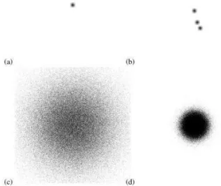
Fig. 1. Sample test images consisting of (a) a single, solitary point-object, (b) a configuration of three single point-objects that is a known problematic configuration, (c) and (d) Randomly generated test images by sampling from a
normal distribution (with different Standard deviations)
III. RESULTS AND EVALUATION
The experimentation was carried out on a Dell 3.6 GHz Pentium 4 system with having 2 GB of RAM. Moreover, the system was running on the RedHat Linux version 2.69 and using the g++ 3.4.2. In the simulation of the experiments, it has been found that, the CPU time for the processing of the images was observed with the exponential time drop. It was also ensured that, none of the other users were logged in the system. The results of the output displayed solitary object consisting of a single point at the centre of the image in figure 1a. The figure 1b consisted of extremely problematic image consisting of the 3 point objects. On the other hand, the randomly generated sets of object were created with having a standard deviation of 0.05 in figure 1c. Finally, figure 1d represents the samples created from the normal distribution with a different standard deviation of 0.05. In addition, each of the input test images has been kept 1000 x 1000 pixels in size. As previously mentioned, distance map algorithm was used; therefore, all of the results have been generated accordingly.
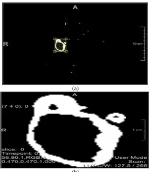
therefore, they all may exhibit same gray level and some shapes for the thyroid images and scanned images of the brain. In the selection of ROI, it is highly mandatory to select the exact region of the analysis. Therefore, it needs to avoid other parts in the image that shall reduce the complexity. Thus, following results were obtained on the run for the ROI.
(a)
(b)
Fig. 2. ROI selection process (a) ROI Selection (b) Extracted Region
In the light of the above mentioned imaging technique, it has been found that, the proposed algorithm has been highly sufficient in reducing the complexity along with producing optimum results.
The second run was to assess the de-noising capability of the algorithm. While considering the medical image processing, it is highly considerable to reduce the noise as much as possible to sharpen the quality of the image. Moreover, noise in the medical imaging can result in the incorrect segmentation of the edge or shape of the region of tissue or an organ. Therefore, the de-noising has been done through median filter. Keeping in mind, the same input image has been used to observe the results. The below mentioned results were obtained:
(a)
(b)
Fig. 3. De-Noising process for the ROI. (a) Original Image (b) Median Filtering
The results obtained from the de-noising process of the ROI by the median filter have been stated in table 1 below. The parameter values of the evaluation have been set as Pixel Value, Volume, Mean and Standard Deviation. Moreover; volume is measured in mm3 and the region of interest has been selected as the brain MRI for the tumour part.
TABLE I. PARAMETER OBTAINED FOR DE-NOISING OF ROI
Parameter Median Filter
Pixel Value 13920
Volume mm3 3079.78
Mean 144.72
Standard Deviation 34.96
From the experimental results, the median filter produced exceptional results, for the de-noising of the image. In a more general perspective, the noise is caused by bit errors during the transmission and the capture of the data. Since, only a small amount of the pixels tend to deviate from the actual points; therefore, the algorithm has been considered to be highly effective in reducing the noise.
Finally, the image was tested for the enhancement of the digital image quality. The work has been analysed on the basis of the histogram equalization method that has been trusted to provide the intensity and grey level enhancement of the image. Therefore the enhancement has been shown in the below mentioned figure:
(b)
Fig. 4. Histogram equalization of brain MRI, (a) Original Image, (b) Enhanced Image
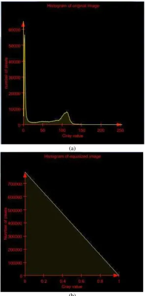
The histogram equalization provides with the normalized range of the image along with uniform intensity of and gray level. Therefore, further elaboration of the histograms has been mentioned below in the figures.
(a)
(b)
Fig. 5. Histogram of images (a) Original Image (b) Normalized Image
In the light of the above mentioned figure, it has been inferred that histogram equalization is one of the most common techniques for enhancing the appearance of the images. In further analysis of the images it has been found that, histogram of the image shows the variation of intensity or gray level. However, it can be avoided by the normalized intensity in the histogram equalization. Therefore, the normalized image provides the uniform intensity throughout the image
After the through considerations of all of the tests that have been conducted to quantify the results, it has been found that, the newly proposed algorithm has been highly effective in terms of the operations that are being evaluated. Therefore, it would not be wrong to state that, the newly derived algorithm has been in high accordance of the optimized procedures. Keeping in mind the optimization is done on the basis of the complexity and the output produced.
IV. CONCLUSION
After the through considerations of all of the operational factors that have been linked with the distance map algorithm; it has been found that, the recently proposed algorithm has been highly effective in meeting the intended goals. Moreover, the computational complexity of the newly developed algorithm has been found to be relatively low as compared to the previous ones. The evaluation of the Taylor series and the comparison to the complexity proposed in the research has posed a significant reduction in the operational norms of the computations. On the other hand, the results also have affirmed the application of the algorithm in critical fields such as medical image processing and others. Thus, it has concluded the fact that, the distance map algorithm has been highly sufficient in addressing the optimum processing of the medical images along with its proper application in the field. Future work is required to improvise the output of the 2D and 3D images. Distance map and other new ideas with new algorithms are possible to make use of the scalar and integer values that are capable of accurately and efficiently calculating the distance transforms of the 2D and the 3D images in a general form and in accurate result. Additionally, future work can be done using other non-linear procedures to be valid and to be used expensively in other applications in the field of image processing, specially, medical images. Future work can be done by applying the proposed algorithm and other modified ones by addressing main concepts of Fractional Calculus for the presentation of derivatives of the non-linear function
which possibly will increase the accuracy and
give better complexity.
REFERENCES
[1] L. Blum, F. Cucker, M. , Shub. and S. Smale, S., . Complexity and real computation. Springer Science & Business Media. 2012.
[2] Nedelcu, V., Necoara, I. and Tran-Dinh, Q. " Computational complexity of inexact gradient augmented Lagrangian methods: application to constrained MPC",. SIAM Journal on Control and Optimization, 52(5), pp.3109-3134 . 2014
[4] R. Miller, ed., Complexity of Computer Computations: Proceedings of a Symposium on the Complexity of Computer Computations, Held March 20–22, 1972, at the IBM Thomas J. Watson Research Centre, Yorktown Heights, New York, and Sponsored by the Office of Naval Research, Mathematics Program, IBM World Trade Corporation, and the IBM Research Mathematical Sciences Department. Springer Science & Business Media. 2013.
[5] A.M. Tillmann, and M.E., Pfetsch,. "The computational complexity of the restricted isometric property, the null space property, and related concepts in compressed sensing" . IEEE Transactions on Information Theory, 60(2), pp.1248-1259.4, 2014
[6] P.J. Dickinson and L. Gijben ," On the computational complexity of membership problems for the completely positive cone and its dual.Computational optimization and applications", 57(2), pp.403-415. 2014
[7] L.Susskind, "Addendum to computational complexity and black hole horizons". Fortschritte der Physik, 64(1), pp.44-48 , 2016.
[8] B. Bognet, F. Bordeu, , F. Chinesta, , A. Leygue, and A. Poitou, "Advanced simulation of models defined in plate geometries: 3D solutions with 2D computational complexity". Computer Methods in Applied Mechanics and Engineering, 201, pp.1-12. 2012.
[9] Y.H., Wang, C.H., Yeh, Young, H.W.V., Hu, K. and M.T., Lo. "On the computational complexity of the empirical mode decomposition algorithm".Physica A: Statistical Mechanics and its Applications, 400, pp.159-167. , 2014.
[10] G., Correa, P. Assuncao, L. Agostini, and L.A., da Silva Cruz, 2012. "Performance and computational complexity assessment of high-efficiency video encoders". IEEE Transactions on Circuits and Systems for Video Technology, 22(12), pp.1899-1909. 2015.
[11] R. Ibsen-Jensen, K. Chatterjee, and M.A. Nowak, "Computational complexity of ecological and evolutionary spatial
dynamics". Proceedings of the National Academy of Sciences, 112(51), pp.15636-15641.2012
[12] A. Arkhipov, and S., Aaronson. "The Computational Complexity of Linear Optics. In Quantum Infomation and Measurement ". Optical Society of America. 2014.
[13] I.M. Bomze, F. Jarre, F. Rendl, Quadratic factorization heuristics for copositive programming. Math. Program. Comput. 3(1), 37–57, 2011. [14] S. Burer. "Copositive programming. In: Handbook of Semidefinite,
Cone and Polynomial Optimization: Theory, Algorithms, Software and Applications", pp. 201–218. Springer, New York, 2012.
[15] P.J.C., Dickinson, M. Dür. "Linear-time complete positivity detection and decomposition of sparse matrices". SIAM J. Matrix Anal. Appl. 33(3), 701–720 2012.
[16] G. Borgefors. " Distance transformations in digital images Computer Vision, Graphics and Image Processing", 34(3):344–371, 1986. [17] A. Barmpoutis, B. Vemuri, and J. Forder. Registration of high angular
resolution diffusion MRI images using 4th order tensors. Med. Image Comput. Comput. Assist. Interv. 10, 908–915. 2007.
[18] E. Paulson, and C., Griffin, "Computational complexity of the minimum state probabilistic finite state learning problem on finite data sets". arXiv preprint arXiv:1501.01300. 2014.
[19] E. D. Andersen and K. D. Andersen. The MOSEK interior point optimizer for linear programming: an implementation of the homogeneous algorithm. In T. T. H. Frenk, K. Roos and S. Zhang, editors, High Performance Optimization, pages 197–232. Kluwer Academic Publishers, 2000.