A discourse on entanglement and its detection in finite dimensions

(1)

A Discourse on Entanglement and its

Detection in Finite Dimensions

Thiago de Oliveira Maciel

(2)

A Discourse on Entanglement and

its Detection in Finite Dimensions

Thiago de Oliveira Maciel

Orientador:

Prof. Dr. Reinaldo Oliveira Vianna

Dissertação apresentada à UNIVERSIDADE FEDERAL DE MINAS GERAIS - UFMG, como requisito parcial para a obtenção do grau de MESTRE EM FÍSICA.

(3)

Dedicate

(4)

(5)

Agradecimentos

Não há como não agradecer, primeiramente, à minha família: a meu pai Ademar e à minha mãe Nara, eles são, simplesmente, os melhores pais que eu poderia ter; à minha irmã Velise, que — graças à ela — pude ir e voltar todos os dias da universidade; à minha irmã Taísa, que me ajuda tanto — nem sei se um dia conseguirei retribuir tudo (cf.esta dissertação escrita toda em inglês: obrigado, mana) —; às minhas tias (Delourdes e Izabel) e tios (Paulo e Sérgio, do lado do pai e Jorge, por parte da mãe), primas (Ceres, Cibele, Jaqueline, Caroline, Gabriela, Daniele, Pâmella e, agora, Gisele), primos (Bruno, Charles, Fábio, Alex, Deivid, Michel, Marcos e, agora, Marcus), agregados e agregadas — que geram todo o meu contexto familiar que me faz ser quem sou e onde as bases para o que ainda posso ser foram construídas — e, claro, ao meu avo Mário Gaspar Maciel: a quem dedico esta dissertação.

Em especial, agradeço ao pessoal do Infoquant (Reinaldo, André Tanus, Debarba e Fernando) e asladiesegentlemen(Geraldo, Campô, Mário Mazzoni, Michelle, Ana Paula, Monique e Luciana Cambraia), mas, independente de qualquer coisa, sempre serei grato aos meus amigos e amigas, que sempre tento cultivar da melhor forma possível: Geraldo, Campô, André Tanus, André Arruda, Michelle, Debarba, Fernando, Ana Paula, Jaque, Ingrid, Julia, Luciana Cambraia, Monique, Mateus, Marco Túlio, Érico, Gláucia, Amanda, Junior, Hobbit, Léo, Gabi, Gabi, Denise, Wanderson, Alex Bueno, Gustavão, Marina, Breno Rotelli, Simone Boff, Isabel Sager, Badaia, Bárbara morena, Bárbara ruiva, Camila, Farley, Palhacinho, Guilherme Almeida, Guilherme (André Matos), Hayssa, Lígia, Lídia, Emílson, Henrique Elias, Lilí, Peter Jaques, Zé Geraldo, Adriani Simonete, Narciso Hansen, Linei Rocha, Reinaldo Portanova, Atos e os Bandidosi. Sem a ajuda do meu amigoπii, não saberia da minha primeira oportunidade de bolsa de iniciação científica com o Reinaldo, portanto, agradeço a ele por isso. Agradeço, também, a Izabella Amim Gomes: que conheço há uns dez anos e por quem tenho um carinho muito especial.

Separo um parágrafo para agradecer a Cyntia, que — na falta de verbetes adequados — digo que preenche os espaços da minha vida com belíssimos interlúdios.

Agradeço, também, ao meu professor e amigo Mário Mazzoni: grande parte do que aprendi sobre física fora ensinado por ele. Também, ao Sebastião

i_{Enumerar pessoas é sempre uma tarefa inglória, perdoem-me caso tenha deixado de citar} alguém.

(6)

de calcular traços de produtos de operadores hermiteanos.

E, claro, agradeço ao meu orientador, professor e amigo Reinaldo Oliveira Vianna: sem a oportunidade de trabalhar com ele, nenhuma palavra estaria escrita neste discurso. Obrigado por me dar a oportunidade de enxergar a mecânica quântica dessa belíssima forma e que, hoje, gera esta dissertação.

(7)

Abstract

We explore procedures to detect entanglement of unknown mixed states, which can be experimentally viable. The heart of the method is a hierarchy of semi-definite programs, which provides sufficient conditions to entanglement. Our numerical investigations indicate that the entanglement is detected with a cost which is much lower than full state tomography. The procedure is ap-plicable to both free and bound entanglements and involves only single copy measurements. The discourse involves density matrices and its properties, quantum manipulations, entanglement and its detection.

Keywords

(8)

(9)

Resumo

Desenvolvemos um método a fim de explorar a detecção do emaranhamento em estados desconhecidos sem tomografia completa. O coração do método está na hierarquia de programação semi-definida. Temos evidências numéricas que indicam que detectar emaranhamento com informação incompleta é possível e tem um custo menor que uma tomografia completa de estado. O método é aplicável tanto ao emaranhamento livre, quanto preso e en-volve medições simples. O discurso aborda matrizes densidades, operações quânticas, caracterização e medição de emaranhamento.

Palavras-chave

(10)

List of Figures

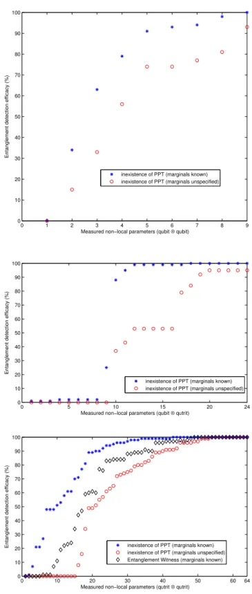
5.1 Fraction of success of entanglement detection against the number of measured non-local parameters —cf.Eq. (5.4)—, for a sample of 104_{random NPT states, using the approaches described in Eqs.} (5.5) and (5.6), for two qubits, one qubit and one qutrit, and two qutrits. For two qutrits, we also show the results using the EW (Eq. (5.8)). . . 60 5.2 Fraction of success of entanglement detection against the number

of measured MUB projectors (cf.Eq. (5.1)) , for a sample of 104 random NPT states, using the approaches described in Eq. (5.5) (Peres-Horodecki criterion), for two qubits (top), and Eqs. (5.5) and (5.8) (EW) for two qutrits (bottom). . . 64 5.3 Fraction of success of entanglement detection against the number

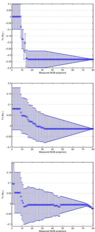
of optimalprojectors (cf.Eq. (5.1) and Table5.3) , for a sample of 104random NPT states, using the approach described in Eq. (5.5) (Peres-Horodecki criterion), for the 2⊗3 system. . . 65 5.4 Estimated EW with its error bar — Eq. (5.8) — for 3 particular

two-qutrit states: (top) Werner state with β=−1, (middle) Werner state withβ=−0.37, (bottom) Horodecki bound entangled state withλ=3.9. In each case, the exact value fortr(Wρρ)corresponds

(13)

List of Tables

5.1 Complete bases of observables in Hilbert spaces of dimensions 2⊗2, 2⊗3 and 3⊗3. Each two-particle observable is the tensor product between one operator of the first line by one operator of the first column. . . 62 5.2 Five maximally commuting classes of observables (cf.Table5.1) for

two qubits. The common eigenvectors of each class form a set of MUBs. . . 62 5.3 Twelve maximally commuting classes of observables (cf.Table5.1)

for qubit⊗qutrit. . . 63 5.4 Ten maximally commuting classes of observables (cf.Table5.1) for

two qutrits. The common eigenvectors of each class form a set of MUBs. . . 63

(14)

(15)

CHAPTER

1

Preface: why do we study

entanglement?!

“Entanglement is not one but rather the characteristic trait of quantum mechanics”.

- Erwin Schrödinger

One of the challenges of understanding nowadays physics is that some of the concepts seem quite abstract when we are discussing about microscopic objects outside the realm of everyday experience. Conventional knowledge holds that quantum mechanics is hard and tough to learn: which is more or less correct — often overstated though —. However, the necessity of abandoning conventional ways of thinking about the world and finding a radically new way — thequantum mechanicalway — may be understood by any curious person willing to spend some mathematics and time concentrating hard. Conveying that understanding is the purpose of this discourse, in particular, we focus on — as Schrödinger said —thecharacteristic trait of quantum mechanics: entanglementi. This exclusive property of quantum systems — which keeps coming back to haunt us — leads the main road of the discourse.

The standard explanation is based on the historical development of quantum mechanics. During that time there were a series of crises to describe the micro-scopical world in physics. The pattern was that each time some experimental fact would be noticed that seemed hard to explain with the old “classical” way of viewing the world. Each time, physicists would bandage over the old classical thinking with anad hocbandaid. This happened over and over again until, in the mid-1920s, the sick patient of classical physics of micro-scopical world finally keeled over completely and was replaced with the new framework of quantum mechanics.

(16)

The problem with this style of explanation, and what makes it confusing, is that none of those early crises was entirely clearcut. In each case, there were physicists who argued that the new experimental results could be explained pretty well with a conventional classical picture.

Imagine one tossing a coin and checking whether is heads or tails. This process of figuring out whether the coin is heads or tails is what physicists call ameasurement process. In physicists’ language, what is going on when we look at the coin is that we aremeasuringa two-valued orbinary property of the coin. This usage of the term measurement is somewhat different from everyday usage, where,e.g., we might measure something with a ruler. But the basic idea is the same: a measurement is a process that determines a physical property — whether it be the length of an object, or the side a coin has landed —.

All this language may seem pedantic: we are just looking at a coin! But it comes in handy when we move from the conventional concepts to standard knowledge. At this point, looking to the quantum mechanics scenario, it is worth quoteii_{Reinaldo Vianna: “In the end, what really matters is the ‘click’} on the detector.”. We believe that no one will look to quantum mechanics in a ‘spooky’ way following this spirit.

The present-day entanglement theory has its roots in the key discover-ies: quantum cryptography with Bell theorem; quantum dense coding and quantum teleportation — including teleportation of entanglement of EPR pairs (so-called entanglement swapping) —. All such effects are based on entanglement and all of them have been demonstrated in pioneering experi-ments. In fact, all these results — including the idea of quantum computation — were a basis for a new interdisciplinary domain calledquantum information:

which have entanglement as a central notion.

Although the reason why we study entanglement is the outstanding applications of this property as resource, it is still a property of quantum compound systems: which needs to be studied carefully and deeply. We will dissect it keenly — with aid of powerful mathematical tools —.

To explore the subject in this keenly fashion, we assume that the reader has the standard lore in quantum mechanics. One remark should be done though: most of the material here has been presented before — this is true for all the literature review and most of the original work —. We just fit it in the main road.

Now, let us explain the road to entanglement presented here in this discourse. In the chapterNice to meet you, density matrix!, we intent to expose and unravel aspects of a density matrix which is forgotten in the standard lore: the concepts of convex sets and positivity of Hermitian matrices.

In the chapterLet entanglement be your puppet: manipulations of quantum states, we gave a unified mathematical representation for quantum manipula-tions. We are pretty sure that — after reading this chapter — the reader will be able to comprehend a vast part of the nowadays literature in the subject.

In the chapterEntang’ what?! Entanglement as a quantum property of com-pound systems, we present entanglement as a property in its full glory, with

(17)

aid of separability criterions, entanglement witness, (un)decomposable maps and describe how we characterize entanglement in a numerical approach.

Finally, equipped with all mathematical tools of the previous chapters, in the last one,A ‘click’ on the detector: measuring entanglement, we make use of them and present our — Thiago O. Macielet al. — work on the subject: checking entanglement with incomplete information about the state —cf.[1]

—.

(18)

(19)

CHAPTER

2

Nice to meet you, density

matrix!

“[...] the most universal picture which remains after the details are forgotten is that of a convex set.”.

- Bogdan Mielnik

Following the spirit of this discourse, we will start the discussion of properties of the object which we used to describe quantum states: the density matrix. One might be satisfied with the standard lore of the subject [2,3]iin

the context of quantum mechanics — but we will explore a little bit furtherii —. Onebona fidedensity matrix should satisfy the following conditions:

(i) Hermitian, ρ=ρ†; (2.1)

(ii) positive semi-definite, ρ≥0; (2.2)

(iii) normalized, tr(ρ) =kρk1=1. (2.3)

But the trace one positive semidefiniteness of the density matrix ρ yields (mathematical) properties which should be unraveled to a careful reader. We start exploring the convex properties of the set of states and, then, go through the conditions (i) and (ii): whereas (ii)implies (i) for complex Hermitian matrices.

2 .

1 The space of density matrices as a convex set

Let us state some general facts and definitions (cf.[5]). There is a restriction

that arises naturally in quantum mechanicsiii_{: the states set must be a}_convex set. A set in which one may form ‘mixtures’ of any points in the set.

i_{And so many others.}

(20)

In a geometric point of view, the mixture of two states may be defined as one point on the segment of the straight line between the two points that represent what we want to mix. In a convex set, all mixtures of this type generates one state belonging to the same set. But, before we see how this restricts the set of the states, we must define what we mean bystraight lines.

Anaffine spaceis just like a flat Euclidean spaceEN_{of dimension}_N_{, except}

that no special choice of origin is assumed. Thus, onestraight linethrough the two pointsρ1andρ2is defined by

ρ= p1ρ1+p2ρ2, p1+p2=1. (2.4)

If we choose one origin inρ0, we see that this generates one plane spanned by the vectorsρ1−ρ0andρ2−ρ0. Then, oneK-dimensional plane is obtained by takingK+1 generic points (withK<_N_{). We call this plane as a}_hyperplane_.

ForK=N, we describe the entire spaceEN_.

Anaffine mapis a transformation that takes lines to lines and preserves the relative length of line segments lying on parallel lines,i.e., a linear transform-ation described by one matrixΛ_{with a translation along a constant vector}_σ

(Λ_ρ₊_{σ) where}Λ_{is an invertible matrix.}

We define a subset of this affine one as aconvex setif, for any pair of points ρ1andρ2belonging to the set, it is true that themixtureρbelongs to the set also,i.e.,

ρ= p1ρ1+p2ρ2, p1+p2=1, p1,p2≥0. (2.5)

The requirement p1,p2 ≥ 0 restrictsρ to belong to the segment of the line lying between the pair of points. The generalization to more points follows from the definition.

We used an affine space as the ‘container’ for the convex sets since con-vexity properties are preserved by general affine transformations, which are common in quantum mechanics.

Given any subset of the affine space, we define theconvex hullof this subset as the smallest convex set that contains the set. The convex hull of a finite set of points is called aconvex polytope. if we take p+1 points that are not confined to any(p−1)-dimensional subspace, then the convex polytope is called ap-simplex,i.e.,

ρ=p1ρ1+· · ·+ppρp, p

∑

i=1

pi=1, pi≥0. (2.6)

Thedimensionof a convex set is the largest number Nsuch that the set contains anN-simplex. A closed and bounded convex set that has an interior is known as aconvex body. Convex bodies always contain some special points that cannot be obtained as mixtures of other points: these points are called pure points, while non-pure points are calledmixed.

Let us quote two useful theorems:

(21)

2.1. The space of density matrices as a convex set

Theorem2(Carathéodory [7]). If X is a subset ofRd_{, then any point in the convex} hull of X can be expressed as a convex combination of at most d+1points in X.

Thus, any point ρ of a convex body S may be expressed as a convex combinationof pure points,i.e.,

ρ=

p

∑

i=1

piρi, p

∑

i=1

pi =1, pi≥0, p≤d+1. (2.7)

TakeL(H)as the space of linear Hermitian operators onH: this is a real vector space of dimensiond=N2−1. The setL+(H)of positive operators is

a convex cone in this space. The set of strictly positive operators is denoted L++(H). It is an open set inL(H)and is a convex cone, also. We will find

much use for the concept ofconvex functions. If f is a map ofL(H)into itself, we say f isconvexif

f((1−α)ρ+ασ)≤(1−α)f(ρ) +αf(σ) (2.8) for allρandσ∈ L(H)and 0≤α≤1. If f is continuous, then f is convex if, and only if,

f

ρ+σ 2

≤ f(ρ) +₂ f(σ) (2.9)

for all ρ andσ. We say f ismonotone if f(ρ) ≥ f(σ)whenever ρ ≥ σ,i.e., ρ−σ≥0 is positive semidefinite.

As ρ is Hermitian, any density matrix can be diagonalized: the set of density matrices that are diagonal in a given basis{|eii}can be written as

ρ=

N

∑

i=1

λi|eiihei|, ρ|eii=λi|eii and N

∑

i=1

λi =1. (2.10)

This set is known aseigenensemble, or as theeigenvalue simplexiv. It forms a particular(N−1)-dimensional cut through the set of density matrices — and every density matrix are placed in some eigenvalue simplex —.

Therankof a point in a convex set is the minimum numberrof pure points that are needed to express it as a convex combination of pure states. Thus, a density matrix of matrix rankrmay be written as a convex sum of no less thanrprojectors — obviously, when diagonalized —. Hence, the maximal rank of a mixed state is equal toN, which is much less than the upper bound N2given by the Carathéodory’s theorem2.

But this is not every possible mixture,e.g., the maximally mixed stateρ⋆

may be obtained as a mixture of pure states by setting equal weights. We may obtainρ⋆ in many other ways. A similar non-uniqueness afflicts all mixed

states: interestingly, this may be expressed in a precise way as follows:

Theorem3(Schrödinger’s mixture theorem [8]). A density matrixρ, having the diagonal form

ρ=

N

∑

i=1

λi|eiihei|,

(22)

may be written in the form

ρ=

M

∑

i=1

pi|ψiihψi|, M

∑

i=1

pi=1, pi ≥0

if, and only if, there exist a unitary M×M matrix U such that

|ψii= √1_p i

N

∑

j=1

Uij p

λi|eii.

Here, all states are normalized to unit length but they need not be orthogonal to each other.

2 .

2 Positive Semidefinite Matrices

The theory of positive definite matrices, positive definite functions and positive linear maps is rich in content. It offers many beautiful theorems that are simple and yet ingenious in their proof, diverse as well powerful in their application. We start with a glimpse of some of the basic properties of positive matrices. This will lead us to main road of the line of thinking followed through the discourse. We will bring mathematical tools in their full glory to dissect the desired properties in the quantum context.

2 .

1 Characterizations

LetHN_{be the}_N_{-dimensional Hilbert space}_CN_{. The inner product between}

two vectors|ψiand|φiis written ashψ|φiv. We denote byL(H)the space of all linear operators onH— sometimes, just a subspace: the space ofN×N matrices of complex entries —. Every elementρ ofL(H) can be identified with its matrix with respect to the standard (canonical) basis{|ii}ofCN. We sayρispositive semidefiniteif

hψ|ρ|ψi ≥0 for all |ψi ∈ H, (2.11) andpositive definiteif, in addition,

hψ|ρ|ψi>0 for all _|_ψ_{i ∈ H}. (₂.₁₂)

A positive semidefinite matrix is positive definite if, and only if, it is invertible. For the sake of simplicity, we use the termpositive matrix for a positive semidefinite — or a positive definite — matrix. Sometimes, if we want to emphasize that the matrix is positive definite, we say that it isstrictly positive. We use the notationρ≥0 to mean thatρis positive andρ>0 to mean it is

strictly positive.

There are some conditions that characterize positive matrices. Some of them are listed below.

(23)

2.2. Positive Semidefinite Matrices

(i) ρis positive if, and only if, it is Hermitian —i.e.,ρ=ρ†— and all its eigenvalues are nonnegative;ρis strictly positive if, and only if, all its eigenvalues are positive;

(ii) ρis positive if, and only if, it is Hermitian and all its principal minors are nonnegative; ρ is strictly positive if, and only if, all its principal minors are positive;

(iii) ρ is positive if, and only if, ρ = AA† for some matrix A; ρ is strictly positive if, and only if, A is nonsingular;

(iv) ρis positive if, and only if,ρ=T†Tfor some upper triangular matrixT. Further,Tcan be chosen to have nonnegative diagonal elements. Ifρis strictly positive, thenTis unique. This is calledCholesky decompositionof ρ;ρis strictly positive if, and only if,Tis nonsingular;

(v) ρis positive if, and only if,ρ= A2for some positive matrixA. Such aA is unique. We write A=ρ1/2and call it the (positive) square root ofρ; ρis strictly positive if, and only if, Ais strictly positive;

(vi) ρis positive if, and only if, there exist|ψ1i, . . . ,|ψni ∈ HNsuch that

ρij≡

ψi ψ_j

;

ρ is strictly positive if, and only if, the vectors ψ_j

, 1 ≤ j ≤ n, are linearly independent.

To illustrate the last condition, let|ψ1i, . . . ,|ψnibe anynvectors in any

Hilbert space. Then, theN×Nmatrix

G(|ψ1i, . . . ,|ψni)ij≡

ψi ψ_j

(2.13)

is positive — being of the formAA†—. It is strictly positive if, and only if, |ψ₁i, . . . ,|ψniare linearly independent. The matrixGis calledGram matrix

associated with the vectors|ψ1i, . . . ,|ψni.

2 .

2 Some theorems

In this section, we present some theorems on positive matricesvi_{. Some} concepts presented here are not that common in quantum literature — but may be useful at some point —. One remark should be done though: we will not make use of these following theorems — in this section and in the next one —- explicitly in this discourse. We present and illustrate them to enforcethe symmetry conditions imposed by positivity in Hermitian matrices. Positive matrices are one special kind of matrix: which will be clear in the last chapterA ‘click’ on the detector: measuring entanglement.

Letρbe a positive operator onH. IfXmaps a Hilbert spaceHintoH′_,

then the operatorXρX†onH′_{is positive also. On the other hand, if}_X_{is an}

invertible operator — andXρX†is positive —, thenρis positive.

(24)

Take ρ andσ: two operators on L(H). We say that ρ is congruentto σ (and writeρ∼σ) if there exists an invertible operatorXonL(H)such that σ =XρX†. Congruence is an equivalence relation onL(H). IfXis unitary, we sayρisunitarily equivalenttoσ(and writeρ≃σ).

Ifρis Hermitian, theinertiaofρis the triple of nonnegative integers

In(ρ)≡(π(ρ),ζ(ρ),ν(ρ)), (2.14)

where π(ρ),ζ(ρ) and ν(ρ) are the number of positive, zero and negative eigenvalues ofρ(counted with multiplicity).

TheSylvester’s law of inertia[11,12] says thatIn(ρ)is a complete invariant for congruence on the set of Hermitian matrices —i.e., two Hermitian matrices are congruent if, and only if, they have the same inertia —.

Let H′ be a subspace ofH and let Pbe the orthogonal projection onto H′_{. If we choose an orthonormal basis in which}_H′ _{is spanned by the first}_k

vectors, then we can write an operatorρonHas a block matrix

ρ=

ρ11 ρ12 ρ21 ρ22

and

PρP=

ρ₁₁ 0

0 0

.

IfXis the one-to-one map ofH′ _into_H_{, then}_X_ρ_X†₌_ρ

11. We say thatρ11is thecompressionofρtoH′_.

If ρ is (strictly) positive, then all its compressions are (strictly) positive. Conversely, if all the principal subdeterminants ofρare nonnegative, then the coefficient in the characteristic polynomial ofρalternate in sign. Hence — by theDescartes’ rule of signsvii—ρhas no negative root.

Takeρ[j]denoting thej×j(for 1≤j≤N) block in the top left corner of

the matrixρ. We call this theleading j×jsubmatrix ofρand its determinant, subdeterminant. If all the leading subdeterminants of a Hermitian matrixρ are positive, thenρis strictly positiveviii. Positivity of other principal minors follows as a consequence.

We denote byρ⊗σthe tensor product of two operatorsρandσ — acting possibly on different Hilbert spacesHAandHB—. As we already know from

standard quantum loreix_{, if}_ρ_and_σ_{are positive, then}_ρ_⊗_σ_{is positive also.} IfρandσareN×Nmatrices, we writeρ◦σfor their entrywise product —i.e., for the matrix which the entries are given byρijσij—. We call thisSchur

vii_{The rule states that if the terms of a single-variable polynomial with real coefficients are} ordered by descending variable exponent, then the number of positive roots of the polynomial is either equal to the number of sign differences between consecutive nonzero coefficients, or is less than it by a multiple of2. Multiple roots of the same value are counted separately.

viii_{The example}_ρ₌ 0 0 0 −1

is a clear example that non-negativity of the two leading subdeterminants is not adequate to ensure positivity ofρ

(25)

productx. Ifρandσare positive, the so isρ◦σ. One way of seeing this is by observing thatρ◦σis a principal submatrix ofρ⊗σxi.

TakeρandσHermitian — or positive — operators, then the sumρ+σis positive also; their productρσis, however, Hermitian if, and only if,[ρ,σ] =0: i.e.,ρandσcommute. Let us take thesymmetrized product, which reads

Υ₌_ρσ₊_σρ. ₍2.15)

Now, if bothρandσare Hermitian, thenΥ_{is Hermitian also. However, if}

ρandσare positive, thenΥ_{need not be positive:} _e.g._{, the matrices}

ρ=

1 0 0 α

and σ=

1 β

β 1

are positive ifα>0 and 0<_β<1, butΥ_{is not positive when}_α_{is close to}

zero andβis close to one. The fact that ifΥ_{is positive and}_ρ_{strictly positive,}

thenσ is positive might be considered surprising: that is why we need to clarify.

Proposition4. Let ρ andσ be Hermitian and suppose ρ strictly positive. If the symmetrized productΥ₌_ρσ₊_σρis (strictly) positive, thenσis (strictly) positive.

Proof. Choose an orthonormal basis in whichσis diagonal:i.e.,diag(ς₁,· · ·,ςn).

ThenΥ_ii₌_2ς_i_ρ_ii_{. Now, observe that the diagonal entries of a (strictly) positive}

matrix are (strictly) positive.

An amusing corollary of Proposition4is a simple proof of the operator monotonicity of the mapρ7→ρ1/2on positive matrices.

If ρ andσ are Hermitian, we say that ρ ≥ σ ifρ−σ ≥ 0; andρ > _σ if

ρ−σ>0.

Proposition5. Ifρandσare positive andρ>_σ_{, then}_ρ1/2>_σ1/2

Proof. Using the identity

ρ2−σ2= (ρ+σ)(ρ−σ) + (ρ−σ)(ρ+σ)

2 , (2.16)

ifρ and σ are strictly positive, then ρ+σ is positive also, so, ifρ2−σ2 is positive, thenρ−σis positive — by Proposition4—.

Remember that ifρ≥σ, then we not always haveρ2>_σ2_:_e.g._{, consider}

ρ=

2 1 1 1

and σ=

1 1 1 1

.

x_{Also called the}_{Hadamard product}_. xi _ρ

ij◦σij

ij=

ρij⊗σkl

kl

(26)

2 .

3 Block matrices

In pursuit of properties yielded by (non-)separable density matrices, the study of block matrices arises as by-product. Although not very common in quantum literature, we present some useful theorems.

We will see that simple 2×2 block matrices play remarkable role in the study of positive matrices.

Let ρbe a block matrix with entries A,B,Cand D, N×Nmatrices: as

ρ =

A B C D

. So,ρ is an element ofL(H2N₎ _{— or}_L₍_HN_{⊕ H}N₎ _{—. We}

will see that several properties of ρ can be obtained from those of a block matrix in whichAis one of the entries.

We denote A=UP for thepolar decompositionof A, whereUis unitary andPis positive.Pcan be readP= (A†A)1/2: this is called thepositive part— or theabsolute value— ofAand is written as|A|. We haveA†=PU†and

|A†|= (AA†)1/2= (UP2U†)1/2=UPU†.

A is said to be normal if AA† = A†A. This condition is equivalent to UP=PUand|A|=|A†|.

We write A = USV for singular value decomposition (SVD) of A, where U andV are unitary and S is diagonal with nonnegative diagonal entries s₁≥ · · · ≥sN: these are the singular values ofA— or the eigenvalues of|A|

—.

The symbol kAkwill denote, in this section, the norm of Aas a linear operator on the Hilbert spaceL(H),i.e.

kAk ≡ sup

k|ψik=1k

A|ψik= sup

k|ψik≤1k A|ψik.

It is easy to see thatkAk=s₁.

Some important properties of this norm are the followingxii_:

kAB_{k ≤ k}A_kkB_k; (2.17) kAk=

A

†

; (2.18)

kAk=kU AVk, (2.19) for all unitaryUandV. This last property is calledunitary invariance. Finally,

A

†_A

=kAk

2_. ₍₂_.₂₀₎

There are other norms onL(HN₎_{that satisfy the first three properties. It}

is the condition (2.20) that makes the operator normk·kvery special. We sayAiscontractive, orAis acontraction, ifkAk ≤1.

Proposition6.The operator A is contractive if, and only if, the operator

₁

A A† 1

(27)

Proof. Let A=USV, then

₁

A A† 1

=

₁

USV V†SU† 1

=

U O

O V†

₁

S S 1

U† O

O V

This matrix is unitarily equivalent to

₁

S S 1

, which in turn is unitarily equivalent to the direct sum

₁

s₁ s1 1

⊕

₁

s2 s2 1

⊕ · · ·

₁

sN

sN 1

,

where s1,· · ·,sN are the singular values of A. These 2×2 matrices are all

positive if, and only if,s₁≤1 (i.e.,kA_{k ≤}1).

Proposition7. Take A and B positive matrices, then the matrix

A X

X† B

is

positive if, and only if, X= A1/2KB1/2for some contraction K.

Proof. Assume first that AandBare strictly positives. Thus allow us to use the congruence

A X

X† B

∼

A−1/2 O O B−1/2

A X

X† B

A−1/2 O O B−1/2

=

₁

A−1/2XB−1/2 B−1/2XA−1/2 1

.

LetK= A−1/2XB−1/2, then by Proposition6, this block matrix is positive if, and only if,Kis a contraction. This proves the proposition when AandB are strictly positive. The general case follows by continuity argument.

One may see that, from Proposition7, if

A X

X† B

is positive, then the

range ofXis a subspace of the range of Aand the range ofX†is a subspace of the range ofB. The rank ofXmay not exceed either the rank ofA, or the rank ofB.

Theorem 8. Let A and B be strictly positive matrices, then the block matrix

A X

X† B

is positive if, and only if, A≥XB−1X†. Proof. Using the congruence

A X

X† B

∼

₁

−XB−1

O 1

A X

X† B

₁

O −B−1X† 1

=

A−XB−1X† O

O B

.

(28)

Lemma9. The matrix A is positive if, and only if,

A A A A

is positive.

Proof. We may write

A A A A

=

A1/2 O A1/2 O

A1/2 A1/2

O O

,

which is positive being of the formXX†.

Corolarium10. Let A be any matrix, then the matrix

|A| A† A |A†|

is positive.

Proof. Use the polar decomposition A=UP, thus

|A| A† A |A†|

=

P PU† UP UPU†

=

₁

O O U

P P P P

₁

O O U†

,

(29)

CHAPTER

3

Let entanglement be your

puppet: manipulations of

quantum states

“[...] quantum phenomena do not occur in a Hilbert space, they occur in a laboratory”.

- Asher Peres

To acquire the full glory of the entanglement as resource, one definitely needs some manipulations of quantum states and — in some cases — classical com-munication.This chapter intend to give a unified mathematical representation for these manipulations: the so-called Kraus formalism [13–15].

This chapter is organized as follows: first we present a general overview of quantum operations, then we will explore a little bit further and present the whole quantum maps framework — where the knowledge of the content in the appendixIn the toolbox: matrix reshaping and reshufflingis assumed —. Finally, we separate quantum operations in classes where increasing degrees of communication are allowed.

3 .

1 General quantum operations

We can construct the formalism of general quantum operations in two ways [3, 16]. In the former, we have an axiomatic point of view: we restrict ourselves to

a class of linear mapsΛ_{which maps a state}_ρ_{acting on}_H₁_{into ˜}_ρ_on_H₂_,i.e.,

Λ:_L₍_H₁₎_{→ L}₍_H₂₎_{, in addition to some physically motivated constraints}

(30)

the one which can be obtained by combining operations from a certain set of elementary operations. They are both equivalenti_.

In the standard lore of quantum operations, there are basically four types of manipulations:

(O1)Unitary transformations:ρ→UρU†, withUU†=1;

(O2)Adding an uncorrelated ancilla: ̺→ρ⊗σ, withσa density operator;

(O3) Tracing out part of the system: ρ₁ → tr_H₂(ρ) with ρ acting on H=H1⊗ H2;

(O4)Projective measurements and postselection:ρ→∑k_i₌₁PiρPi, withPi

pairwise orthogonal projectors such that∑n_i₌₁Pi=1 withk≤n.

It is easy to see that operations (O1)-(O3) can be represented as trace preserving completely positive maps — or CP-map, for short —. The inverse holds also,i.e., any trace preserving CP-map can be executed by means of the quantum manipulations (O1)-(O3). This result follows from the Stinespring dilation theorem [13,16,18,21].

Now, with aid of the Choi-Kraus representation, any CP-mapΛ_{can be}

written asΛ₍_ρ_{) =}∑_iEiρE†i ∀ρ∈ L(H). The operatorsEiare commonly called

the Kraus operators. For a trace preserving CP-map, we have∑_i₌₁E†_iEi=1,

but, in the case we allow (O4), we need to relax this constraint to∑_iE_i†Ei≤1

and renormalize the stateii_{. Thus we may summarize this as follows (}_cf._[₁₃_]):

Theorem11. A quantum operationΛ_{can be decomposed into operations of the form}

(O1)-(O4) if and only ifΛacts as a CP non-increasing map:Λ(ρ) =∑_iEiρE†i, with

∑_iE†_iEi ≤1.

3 .

2 Positive and completely positive maps

With a carefully study of the previous section, one should be able to get the idea presented in most of quantum protocols in the literature. But there are lots of things to say when dealing with quantum operations. To explore quantum maps in their full glory, we need a consistent framework: that is what we will explain in this section — we remark here that, at this point, one shouldunderstand the content in the appendixIn the toolbox: matrix reshaping and reshuffling—. So, let’s start with the ‘indices juggling’!

We are particularly interested in a class of mapsΛ_{which maps a state}_ρ

acting onHN_{into ˜}_ρ_on_HN_, _Λ_:_L₍_HN₎_{→ L}₍_HN₎_{. So, what conditions need}

to be fulfilled by a mapΛ_{to represent a physical operation?}

As the linearity of quantum mechanics is assumed here in this discourseiii_, our first constraint on Λ _{is that the map should be a linear one,} i.e., we postulate the existence of alinear superoperatorΛ_,

˜

ρ=Λ_ρ _{or ˜}_ρ_m_µ₌Λmµ

nνρnν, (3.1)

i_{It was introduced, in physics, by Kraus [17] — based on an earlier theorem by Stinespring} [18] — and, independently, by Sudarshanet al.[19].Cf.[14] and [20] also.

ii_{We can also maintain}_∑

iEi†Ei=1but allowing postselection on the outcomes ofi.

(31)

3.2. Positive and completely positive maps

where summation over repeated indices is understood throughout this section. One may understand the first equality in Eq. (3.1) as(Λ_ρ_↓₎_,_i.e._{, a}

superop-erator acting on the reshapedρ(as a column vector) and, then, reshaped back to de square form. This form includes inhomogeneous maps also, ˜ρ=Λ_ρ₊_σ

reads

Λmµ

nνρnν+σmµ≡(Λmnνµ+σmµδnν)ρnν=

˜

Λmµ

nνρnν (3.2)

directly from the fact thattr(ρ) =1,i.e., we are dealing with affine maps of density matrices.

Now that we dealt with linearity, we should take into account the preserva-tion of the density matrices properties of the image ˜ρ: (i) Hermiticity; (ii) trace equals one and (iii) positivity. These requirements impose three constraints on the matrixΛ_:

(i) ρ˜=ρ˜† ⇔ Λmµ

nν =

Λ∗_µ_m

νn so

Λ∗₌ΛS_; ₍₃_.₃₎ (ii) tr(ρ˜) =1 ⇔ Λmm

nν =δnν ; (3.4)

(iii) ρ˜≥0 ⇔ Λmµ

nνρnν≥0 when ρ≥0. (3.5)

Which, presented this way, is notthatilluminating.

To unravel these constraints in a clear way, we may reshuffleΛ_{— as in Eq.}

(A.12) — and define thedynamical matrixiv

DΛ≡ΛR so that Dmn

µν =Λmnµν. (3.6)

The dynamical matrixDΛuniquely determines the mapΛ. Which obeys

DaΛ+bΦ=aDΛ+bDΦ, (3.7)

i.e., it is a linear function of the map.

Now we are able to write the three conditions as

(i) ρ˜=ρ˜† ⇔ Dmn

µν =D

†

mn

µν so DΛ=D

†

Λ; (3.8)

(ii) tr(ρ˜) =1 ⇔ Dmn

mν =δnν ; (3.9)

(iii) ρ˜≥0 ⇔ Dmn

µνρnν≥0 when ρ≥0. (3.10)

Which gives us a better picture. The condition (i) holds if, and only if,DΛis

Hermitian; condition (ii) takes a familiar form also:

Dmn

mν =δnν ⇔ trA(DΛ) =1, (3.11)

i.e., the partial trace with respect to the first subsystem is equal the identity operator for the second subsystem; only the condition (iii) needs further explanation.

(32)

This requirement stands for the positivity of the map,i.e.,Λ_{should map}

positive matrices to positive matrices — so (iii) must holds —. Consider the original density matrix be a pure one, so thatρnν=znz∗ν. Then its image will

be positive if, and only if, for all vectorsxm,

xmρ˜nνxµ∗ = xmznDmn

µνx

∗

µz∗ν ≥0. (3.12)

In the usual notation, one reads this equation as

hx|ρ˜|xi=hx|⊗hz|DΛ|xi⊗|zi ≥0. (3.13)

But note that, juggling indices, is an easier way to show the equality. The equations (3.12) and (3.13) mean that the dynamical matrix itself must be positive when acts on product states inHN2_{. This property is called}

block-positivity. Which lead us to the following theorem (cf.[23]):

Theorem12(Jamiołkowski). A linear mapΛ_:_L₍_H_A₎_{→ L}₍_H_B₎_{is positive if,}

and only if, the corresponding dynamical matrix DΛis block-positive.

The converse holds also, since (3.12) is strong enough to ensure that (3.10) holds for all mixed statesρas well.

Some remarks about the positivity condition should be done: first, it is difficult to work with — since must holds forallproduct vectors acting on HN2 _{—; another point is that any quantum state}_ρ _{may be extended by an}

ancilla to a state ρ⊗σ of larger composite system. This simple point lead us to check rather the mapΛ_⊗1remains positive. Since the map leaves the ancilla unaffected, this may seem like a foregone conclusion. Classically it is so, but quantum mechanically it is not. So, we must introduce the concept of K-positivity: aK-positive map is a positive map such that the induced map

Λ_⊗1K, where _L₍_HN₎_{→ L}₍_HN_{⊗ H}K₎, (₃.₁₄)

is positive for k ≥ 1. Λ _{is said}_{a completely positive map} _{if, and only if, is}

K-positive for all k ≥ 1. But, check for all possible extensions looks non-operational, so, let us call the dynamical matrix properties of the map to unravel this. SinceDΛis an Hermitian operator acting onHN

2

, it admits a spectral decomposition

DΛ= r

∑

i=1

λi|ξiihξi| so that Dmn

µν =

N2

∑

i=1

λiΞimn(Ξµνi )∗, (3.15)

whereris the rank ofDλ; the eigenvaluesλi are real and the matricesΞimn

are reshaped vectors inHN2_.

Now we are able to check the positivity of the induced mapΛ_⊗1when it acts on matrices inL(HNK_{) =}_L₍_HN_{⊗ H}K₎_{. We pick an arbitrary vector}_z

nn′

inHNK_{and act with our map on the corresponding pure state:}

˜

ρmm′µµ′ =Λmµ

nνδm′µ′

n′ν′

znn′z∗νν′ =Dmn

µνznm′z

∗

νµ′=

∑

i

λiΞimnznm′(Ξiµνzνµ′)∗.

(33)

Let us pick another arbitrary vector xmm′ and test whether ˜ρ is a positive

operator:

xmm′ρ˜mm′µµ′x∗_µµ′ =

∑

i

λi|Ξimnxmn′znm′|2≥0, (3.17)

which must hold for arbitraryxmm′andzmm′, thus all the eigenvaluesλi must

be non-negative. This leads us to Choi’s theorem:

Theorem13(Choi #2). A linear mapΛ_{is completely positive if, and only if, the}

corresponding dynamical matrix DΛis positive.

It is remarkable that we are able to check complete positiveness of the map by looking to the non-negative eigenvalues of the dynamical matrixv_.

The set of complete positive maps is isomorphic to the set of positive matricesDΛof sizeN2. When the map is trace preserving also, we need to

add the condition (3.11), which implies that tr(DΛ) = N. We may think of

the set of trace preserving completely positive maps as a subset of the set of density matrices inL(HN2₎_{, with a unusual normalization though}vi_.

So, the dynamical matrix is positive if, and only if, it may be written in the form

DΛ=

∑

i

|EiihEi| so that Dmn

µν =

∑

i

Eimn(Eiµν)∗, (3.18)

where the vectors|Eiiare arbitrary to an extent given by Schrödinger’s mixture

theorem. Thus, we arrive at an alternative characterization of completely positive maps. They are the maps that may be written in theoperator sum representation:

Theorem14(Choi #1). A linear mapΛ_{is completely positive if, and only if, it is of}

the form

Λ₍_ρ_{) =}

_∑

i

EiρEi†. (3.19)

This also known as theKrausorStinespring form, since its existence follows from theStinespring dilation theoremvii. The operatorsEi are known asKraus

operators. The map will betrace preservingif, and only if, the condition (3.9) holds, which reads

∑

i

E†_iEi =1. (3.20)

Trace preserving completely positive maps go under various names: determin-isticorproper quantum operations,quantum channels, orstochastic maps. This is the most general class that we need to consider.

The convex set of proper quantum operations is denotedCPN_{. To find}

its dimension, we note that the dynamical matrices belong to the positive cone in the space of Hermitian matrices of size N2 (i.e., N2×N2), which

v_Cf._{[24] for further explanation.}

(34)

has dimension N4(i.e.,N4linearly independent parameters); the dynamical matrix corresponds to a trace preserving map if, and only if, (3.11) holds,i.e., the partial trace is the identity operator, so it is subject toN2conditions. Thus, the dimension ofCPN equals_N4₋_N2.

Since the operator sum representation does not determine the Kraus operators uniquely, we would like to bring it to a canonical form. The problem is quite similar to that of introducing a canonical form for a density matrix: its eigenstates. Such a decomposition of the dynamical matrix was given in Eq. (3.15). A set of canonical Kraus operators may be obtained by settingEi =√λiΞi. Which leads us to the following results:

Definition15(Canonical Kraus form). A completely positive mapΛ_:_L₍_HN₎_→

L(HN₎_{may be represented as}

Λ₍_ρ_{) =}

r≤N2

∑

i=1

λiΞiρΞ†i = r

∑

i=1

EiρE†i, (3.21)

where

tr(E†_i Ej) = q

λiλjξi ξ_j

=λiδij. (3.22)

If the map is trace preserving also, then

∑

i

E†_iEj=1 ⇒

∑

i

λi=d2. (3.23)

IfDΛis non-degenerate, the canonical form is unique up to phase choice

for the Kraus operators. TheKraus rankof the map is the number of Kraus operators that appear in the canonical form and equals the rank r of the dynamical matrix.

As in Eq. (A.7), the operator sum representation may be written as

Λ₌

N2

∑

i=1

Ei⊗E∗i = N2

∑

i=1

λiΞi⊗Ξ∗i. (3.24)

The canonical operator sum representation may be considered as a Schmidt decomposition (A.9) ofΛ_{— with Schmidt coefficients}_λi

schmidt=λi—.

We will continue the discussion of positive maps and the duality mapsvs. states in the next chapter.

In the next subsections we will describe the most common classes of quantum operations in the bipartite caseHA⊗ HB(Alice and Bob) without

loss of generality in the multipartite case. The extension to more parties,e.g., Clarice, David, Eve,etc.viiiis straightforward. We now review these classes of operations: where increasing degrees of communication are allowed [13, 25–27].

(35)

3 .

2 .

1 Local operations

Local operations are the most simple manipulations that we are able to perform. This class is generated by the Kraus operators of the formAi⊗1and

1_⊗_B_i, with∑_iA†_iAi =∑iB†iBi =1. In this case, the parties are not allowed

to communicate and the operations are non-measuring. Blending them, we are able to describe local operations as follows:

Λ₍_ρ_{) =}

_∑

i,j

(Ai⊗Bj)ρ(Ai⊗Bj)†. (3.25)

3 .

2 .

2

1 -local operations

Now communication starts to play a few roles: suppose we allowlocal op-erations and one-way communicationfrom Alice to Bob. Now Alice performs a generalized measurement on her subsystem, with Kraus operatorsAi⊗1,

with∑_iA†_iAi=1. If the result of her operation isi, the operation on the state

acts asix

(Λ_i_⊗1₎₍_ρ_{) = (}_A_i_⊗1₎_ρ₍_A_i_⊗1₎†.

Alice is able to pick up the phonex_{and tell Bob that she found result}_i_{, and,} depending on that outcome, he decides which trace preserving operation (defined by Bji operators with ∑jB†jiBji = 1) he will perform. The indexi

denotes the operation Bob implements depends on the result that he got from Alice. The global state now reads

(Λ_iA_⊗ΛB_ji₎₍_ρ_{) =}

_∑

j

(1_⊗_B_ji₎₍_A_i_⊗1₎_ρ₍_A†

i ⊗1)(1⊗B†ji).

If they continue this protocol on many particles, the total ensemble will change as

ΛAB₍_ρ_{) =}

_∑

i,j

(Ai⊗Bji)ρ(Ai⊗Bji)†. (3.26)

Obviously, postselection for certain i may occur in some terms of this expression. The equation (3.26) describes the local operations and one-way communication. The quantum teleportation protocol is the most famous case of this scheme: where Alice performs a Bell measurement.

3 .

2 .

3

2 -local operations: the paradigm of LOCC

The generallocal operations and classical communication(LOCC) paradigm was first formulated in [28]. Distant parties (in this case we consider Alice and

Bob) are allowed to perform arbitrary local quantum manipulations and communicate classically. Note thatnoquantum communication is allowed, i.e., no transfer of quantum systems between the parties can be done.

ix_{Notice that is a trace decreasing operation — as it will occur only with a certain probability} —.

(36)

The mathematical description of the local operations and two-way com-munication is quite complicated and the notation tends to be cumbersome, but we will try to explain in a clear way. In this situation it is useful to do alternating measurements and communications. We follow the same strategy of1-local, focus on one particular outcome and do the summation at the end. Alice starts the protocol and make her measurement, she findsi₁as result, therefore the main operator here isAi1⊗1. Now she pick up the phone and tells her result to Bob, he will then perform1_⊗_B_j

1(i1)— which is a function of Alice’si1outcome — and communicate his result to Alice. She decides then executeAi₂(i1,j1)⊗1— which is function of Bob’s outcome (which is function of Alice’s first outcome)xi_{—. All these operators satisfy similar normalization} properties (sum the products to identity).

In the end of the LOCC protocol (for the total ensemble) we have

Λ₍_ρ_{) =}

_∑

k

(Ak⊗Bk)ρ(Ak⊗Bk)†, (3.27)

with k={i₁,i2,. . . ,in,j1,j2,. . . ,jn} and

Ak =Ain(i1,i2, . . . ,in−1;j1,j2, . . . ,jn−1). . .Ai2(i1,j1)Ai1 Bk =Bjn(i1,i2, . . . ,in;j1,j2, . . . ,jn−1). . .Bj2(i1,i2,j1)Bj₁(i1).

Postselection can be done also for particular choices ofi₁,i₂, . . . ,in,j1,j2, . . . , jn−1.

3 .

2 .

4 Separable operations

This class of quantum manipulations was considered in [27,29]. Separable

operations are defined as any operation which can be written as

Λ₍_ρ_{) =}

_∑

i

(Ai⊗Bi)ρ(Ai⊗Bi)†, (3.28)

where each Ai andBi are arbitrary operations — measurements included —

with the usual normalization condition∑_i(Ai⊗Bi)†(Ai⊗Bi) =1. It follows

that any LOCC is also separable, but the reverse is generally not true [25].

However, we do have the following theorem (cf.[26]):

Theorem 16. It isalways possible to simulate a separable operation using only LOCC, but with probability possibly smaller than one.

Proof. Suppose Alice and Bob have two sets of operatorsAiandBi such that

∑_i(Ai⊗Bi)†(Ai⊗Bi) =1 and a stateρ. Generally, we have∑i=1Ai†Ai 6=1

and∑_i₌₁B†_iBi 6=1. So we are able to rescale the operators to ˜Ai =aAi and

˜

Bi =bBi so that∑i=1A†iAi ≤1and∑i=1B†iBi ≤1. Alice and Bob then will

perform a LOCC and will obtain two outcomes:kAekB. Their strategy is to

maintain the state only if the outcomes coincide (kA =kB). Without keeping

track of the outcomes,ρis mapped into

Λ₍_ρ_{) =}_N

_∑

i

pi

(A˜i⊗B˜i)ρ(A˜i⊗B˜i)†

tr((A˜i⊗B˜i)ρ(A˜i⊗B˜i)†)

=

∑

i

(Ai⊗Bi)ρ(Ai⊗Bi)†, (3.29)

(37)

with pi≡tr((A˜i⊗B˜i)ρ(A˜i⊗B˜i)†)and N a normalization factor.

3 .

2 .

5 PPT-preserving operations

This class of quantum manipulations does what its name says: maps ancilla PPT states into PPT states. We can follow the Rains’ definition [30, 31],

operationsΛ_{such that the induced map}

1_⊗Λ:_ρ_→Λ₍_ρTB₎TB

is completely positive (with TB stands for partial transposition in the Bob

subsystem). We remark here that all separable operations are PPT-preserving (cf.[16])

h

(A⊗B)ρ(A⊗B)†iTB =h(A⊗(B†)T)ρTB₍_A†_⊗_B₎ixii.

Note that PPT-preserving operations are the first class of operations which can be regarded as non-localxiii_{. The key result on this class is that they may} be implemented probabilistically by means of LOCC when both parties share a specific entangled PPT state. This was first realized in [26] by Cirac et al.. They characterized completely general quantum operations (in particular entangling ones) on bipartite systems by means of a generalized Jamiołkowski isomorphism.

3 .

2 .

6 Entangling operations

The Jamiołkowski isomorphism [23] is an isomorphism between a linear map

from an input space to an output space and an operator defined over the tensor product of these two spaces. This correspondence is useful when the map acts on one part of a bipartite system, but, on compound systems, it is not so clear how to interpret this duality. The physical interpretation came in a very elegant way in [26].

Suppose one have two systems, A and B, each consisting of twod-level subsystems A = A₁,A₂ and B = B₁,B₂ respectively. We will establish an isomorphism between a CP-mapΛ₌Λ_A_1,_B

1 :L(HA1,B1) → L(HA1,B1)and an operator O = OA₁,A₂,B₁,B₂ acting on the total system HA⊗ HB. The

isomorphism reads

O ≡1_A_2,_B

2⊗ΛA1,B1(PA1,A2⊗PB1,B2), (3.30) where Λ_{acts only on the systems} _A₁ _and_B₁_{. Here}_P_A

1,A2 is the projector

on the maximally entangled state|ψiA1,A2 ≡ 1 √ d

d−1

∑

i=0|

iiiA1,A2 (analogously for

PB1,B2). Equivalently, we have

Λ₍_ρ_A_1,_B₁₎_≡d2trA2,B2(OρTA₂,B₂)≡d4trA2,A3,B2,B3(OρA3,B3PA2,A3PB2,B3).

xii_{This equation may be written in more concise way, with aid of the four index notation.}

Cf.the appendixIn the toolbox: matrix reshaping and reshuffling.

(38)

From (3.30) it follows thatOis the result of the action ofΛ_{on two systems}

A₁andB₁which are prepared in a maximally entangled state with two acillary systems.

The second form has an equally simple interpretation: if both parties share a stateO, then they may implement the mapΛ_{probabilistically on a}

certain stateρA1,B1 by simultaneously projecting and postselectingρA3,B3, and O on the maximally entangled states ofA2A3andB2B3with the probability of p = 1_d — where d is the dimension of the Hilbert space —. From this isomorphism one can easily deduce the following correspondences:

1. Λ_{is a separable operation if} _O _{is separable, and conversely} Λ _{is an}

entangling operation ifOis entangled — with respect to A and B —;

2. Λ _{is a PPT-preserving operation if and only if} _OTA ≥ 0. Thus any

PPT-preserving operation may be implemented probabilistically locally with aid of a shared PPT state.

This isomorphism has a large number of applications (cf.[26,32]) which

we will not explore further. A simple application is the classification of global unitaries according to their entangling power on composite systems [33–35]. Entangling power of a unitary is defined as the average entanglement

a unitary creates on product states. WhenΛ_{is a unitary map,}_O _{is a pure}

(39)

CHAPTER

4

Entang’ what?! Entanglement

as a quantum property of

compound systems

“Thus one disposes provisionally (until the entanglement is re-solved by actual observation) of only acommon description of the two in that space of higher dimension. This is the reason that knowledge of the individual systems can decline to the scantiest, even to zero, while that of the combined system remains continu-ally maximal. Best possible knowledge of a whole doesnotinclude

best possible knowledge its parts — and this is what keeps coming back to haunt us.”.

- Erwin Schrödinger

There is no manner to introduce entanglement without a brief historical overviewi_{. Starting with EPR}_gedanken_{experiment [}₃₇_,₃₈_{], from the}₁₉₃₀_’s, entanglement was vastly explored in the scenario of the completeness of quantum mechanics: which was put in solid mathematical grounds in the 1960’s — by the striking works of Gleason [39], Kochen and Specker [40] and

Bell [41,42]. Bell’s work dealt directly with th EPRgedankenexperiment and is of a major importance as it showed that entanglement is incompatible with a certain local hidden variable model (LHV) hypothesis. For deep treatments on Bell’s inequalities,cf.[43,44].

Nowadays, the problem of completeness seems well proposed and consid-erable effort has been put into understanding the mathematical structure of entanglement: which lead us to the spirit of this discourse. The first problem is: given an arbitrary quantum state, determine whether it is entangled, or not.

(40)

The study of this problem came together with the realisation that Bell-like inequalities are pretty weak tests for entanglement. The breakthrough came when notions from convex analysis and C∗-algebrasii were applied to the problem (cf.[46, 47]). We will review these results leading to the general

framework of entanglement witnesses and its dual formulation in terms of positive maps. We introduce the so-called PPT entangled states and relate them to classical problems in linear algebra. The separability problem has been shown to beNP-hard [48], therefore, there is no hope of finding a simple

analytical method and no efficient algorithm which is able to distinguish all entangled states from all separable ones (cf.[49,50]). Thus, interest has grown

in finding good numerical heuristics in tackling the problem in low dimen-sions. We will apply tools from semidefinite programming to the separability problem. In particular, we focus on the work by Brandão and Vianna [51–53].

For reviews of entanglement versus separability problem from different viewpoints,cf.[16,54–61].

4 .

1 Characterizing entanglement

In spite of the fact that violation of Bell-like inequalities reveals that quantum correlations may be greater than classical ones, it will be clear that Bell inequalities are a poor test of non-classical behavior. It is possible to show that, for any entangled pure state shared by an arbitrary number of parties, there exists a Bell inequality which is violated [62,63]. For mixed states, this

story has lots of complications and open problems, but it has been shown that although a state might not violate any Bell-like inequalities, it still may be useful for teleportation — using entanglement as resource — [64,65]. In

other scenarios, there are some states which only violate some inequality after a certain local generalized measurement [66, 67]; other states only show a

violation when multiple copies are measured collectively [68].

So, given the difficulties of check entanglement with inequalities, it is convenient to characterize the set of entangled mixed states with some reason-able mathematical definitions. The advantage of this approach is to have a workable definition of what is entangled — and what is not —.

Let us present the definition of entanglement for bipartite systems — the generalization to multipartite is straightforward —, starting with pure states [69, 70]. Let _H be a Hilbert space such that_H = HA⊗ HB, as we said in

chapterNice to meet you, density matrix!, we denote byHd_{the Hilbert space of}

dimensiondwhich is∼=Cd, thus, let_Hd₌_Hda_{⊗ H}db, where_d₌_d_a×_d_b ≥4,

Definition17. A pure state|ψi ∈ Hd_{shared by two parties, Alice and Bob, is called}

separable if, and only if, it may be written as

|ψi=|ψAi ⊗ |ψBi,

with|ψAi ∈ HAand|ψBi ∈ HB,i.e., belongs to the Cartesian productHA× HB⊂

HA⊗ HB. Otherwise, we call|ψientangled.

A discourse on entanglement and its detection in finite dimensions

A Discourse on Entanglement and its

Detection in Finite Dimensions

Thiago de Oliveira Maciel

A Discourse on Entanglement and

its Detection in Finite Dimensions

Thiago de Oliveira Maciel

Orientador:

Prof. Dr. Reinaldo Oliveira Vianna

Dedicate

Agradecimentos

Abstract

Resumo

Contents

List of Figures

List of Tables

CHAPTER

1

Preface: why do we study

entanglement?!

CHAPTER

2

Nice to meet you, density

matrix!

2

.

1

The space of density matrices as a convex set

∑

∑

∑

∑

∑

∑

∑

∑

∑

2

.

2

Positive Semidefinite Matrices

2

.

2

.

1

Characterizations

2

.

2

.

2

Some theorems

2

.

2

.

3

Block matrices

CHAPTER

3

Let entanglement be your

puppet: manipulations of

quantum states

3

.

1

General quantum operations

3

.

2

Positive and completely positive maps

∑

∑

∑

∑

∑

∑

∑

∑

_∑

_∑

_∑

_∑

_∑

_∑

_∑