C¹ Positive Surface over Positive Scattered Data Sites.

Data Sites

Farheen Ibraheem1*, Malik Zawwar Hussain2, Akhlaq Ahmad Bhatti1

1National University of Computer and Emerging Science, Lahore, Pakistan,2Department of Mathematics, University of the Punjab, Lahore, Pakistan

*farheen.butt@gmail.com

Abstract

The aim of this paper is to develop a local positivity preserving scheme when the data amassed from different sources is positioned at sparse points. The proposed algorithm first triangulates the irregular data using Delauny triangulation method, therewith interpolates each boundary and radial curve of the triangle byC¹ rational trigonometric cubic function. Half of the parameters in the description of the interpolant are constrained to keep up the positive shape of data while the remaining half are set free for users’requirement. Orthogo-nality of trigonometric function assures much smoother surface as compared to polynomial functions. The proposed scheme can be of great use in areas of surface reconstruction and deformation, signal processing, CAD/CAM design, solving differential equations, and image restoration.

1. Introduction

Data measured or amassed from many engineering and scientific fields, is often positioned at sparse points. For example, meteorological measurements at different weather stations [1], density measurements on different positions within the human body, heart potential measure-ments at random points in the diagnosis of various ailmeasure-ments of heart [2], 3D photography, aeronautical engineering and industrial design, structural graph networks [3], graph entropy [4], [5], [6]. A visual model is often required to get a clear understanding of underlying phe-nomena as colossal amount of data is difficult to analyse or communicate a message in raw form. Further, a meticulous visual representation obligates the interpolating function to affirm intrinsic attributes of data like positivity, monotonicity and convexity. Although, tensor prod-uct provides a robust medium for fitting surface to rectilinear data sites, it can not be used to fit a surface over sparse data points. This paper addresses the problem of retaining positivity over scattered data points.

Several approaches have been proposed in literature to address the problem of positivity preserving interpolating surfaces. Amidor [7] surveyed method to interpolate scattered data necessitating from electronic imaging system. The author mainly examined radial basis func-tion method, tetrahedral interpolafunc-tion, cubic triangular interpolafunc-tion, triangle based blending interpolation, inverse distance method and neutral neighbourhood. The difference between

a11111

OPEN ACCESS

Citation:Ibraheem F, Hussain MZ, Bhatti AA (2015) C¹ Positive Surface over Positive Scattered Data

Sites. PLoS ONE 10(6): e0120658. doi:10.1371/ journal.pone.0120658

Academic Editor:Cheng-Yi Xia, Tianjin University of Technology, CHINA

Received:July 12, 2014

Accepted:February 5, 2015

Published:June 9, 2015

Copyright:© 2015 Ibraheem et al. This is an open access article distributed under the terms of the

Creative Commons Attribution License, which permits unrestricted use, distribution, and reproduction in any medium, provided the original author and source are credited.

Data Availability Statement:All relevant data are within the paper.

Funding:The authors have no support or funding to report.

scattered data interpolation and scattered data fitting was also demonstrated in the survey. Cubic and quintic Hermite interpolants were used for preserving monotonicity, positivity and convexity of discrete data by [8]. Piah, Goodman, Unsworth [9] first triangulated the data points by Delaunay triangulation and constructed the interpolating surface consisting of“cubic Bezier triangular patches”. Positivity of data was achieved by imposing sufficient conditions on Bezier ordinates in each triangular patch. The proposed scheme was local andC1continous. Hussain and Hussain [10] arranged the scattered data over a triangular grid to preserve the positivity and monotonicity. The authors used a cubic interpolant with one parameter to inter-polate the boundary of each triangular patch while linear interpolant was used in Nielson side vertex method to obtain radial curves. Final surface patch was obtained by convex combination of interpolants. Positivity and monotonicity was retained by deriving data dependent con-straints on free parameters.C1Quadratic splines and Powell-Sabin splines were used as inter-polating function to tackle the problem of range restricted univariate and bivariate scattered data by Hermann et. al. [11]. The authors obtained a system of inequalities for the gradients and positivity was accomplished by deriving sufficient conditions on this system. AC1local ra-tional cubic Bernstein Bezier interpolatory scheme was proposed by Hussain and Hussain [12] to retain positivity of scattered data. In each triangular patch, inner and boundary Bezier ordi-nates were confined for positivity. If in any triangular grid, Bezier ordiordi-nates failed to attain pos-itive shape of data, then these were varied by the weights described in formation of rational cubic Bernstein Bezier interpolant. Sarfraz et. al. [1] established a localC1approach to keep up the positivity of scattered data positioned over a triangular domain. They employedC1rational cubic function with four parameters in Nielson side vertex technique to formulate the interpo-lating surface. Two of the four parameters were constrained for positivity.

Although several approaches have been proposed to retain the positivity of data, little atten-tion has been paid towards the use of trigonometric basis funcatten-tion. This paper develops a posi-tivity preserving scheme for scatter data by takingC1rational trigonometric function [13] into account. Delaunay triangulation method has been used to place scatter data as vertices of trian-gle. Nielson side vertex method [14] has been employed in each triangle to construct triangular patches. TheC1rational trigonometric cubic function [13] with four parameter has been used for the interpolation along boundary and radial curve of the triangle. Positivity is attained by deriving data dependent condition on half of the parameters in the description ofC1rational trigonometric cubic function [13].

The remainder of the paper is formulated as: Section 2 reviews the ratonal trigonometric cubic function [13]. Nielson side vertex method [14] to formulate triangular patches is detailed in Section 3. Positivity preserving algorithm is developed and explained in Section 4. Section 5 demonstrates the developed algorithm and presents graphical results. Section 5 summarizes this research and draws conclusion.

2. Rational Trigonometric Cubic Function

Let {(xi,yi),i= 0,1,2,. . .,n−1} be the given set of data points defined over the interval [a,b]

wherea=x0<x1<x2<. . .<xn=b. A piecewise rational trigonometric cubic function is

de-fined over each subintervalIi= [xi,xi+1] as

SiðxÞ ¼

piðyÞ

qiðyÞ

piðyÞ ¼ aifið1 sinyÞ

3

þ b_ifiþ 2hiaidi

p

sinyð1 sinyÞ2

þ g_ifiþ1

2hididiþ1

p

cosyð1 cosyÞ2þd_ifiþ1ð1 cosyÞ 3

qiðyÞ ¼ aið1 sinyÞ

3

þb_isinyð1 sinyÞ2þg_icosyð1 cosyÞ2þd_ið1 cosyÞ3

where

y¼p

2

x xi

hi

;hi ¼xiþ1 xi; i¼0;1;2; :::;n 1

The rational trigonometric cubic function (Eq 1) satisfy the following properties:

SðxiÞ ¼fi;Sðxiþ1Þ ¼fiþ1;S0ðxiÞ ¼di;S0ðxiþ1Þ ¼diþ1: ð2Þ

dianddi+1are derivative at the endpoints of the intervalIi= [xi,xi+1].αi,βi,γiandδiare the

free parameters. The following result has been proved in [13].

Theorem 2.1The C1piecewise rational trigonometric cubic function preserve the positivity of positive data if in each subinterval Ii= [xi,xi+1], the parametersβiandγisatisfy the following

suf-ficient conditions

b_i¼uiþmax 0;

2hidiai

pfi

;ui>0;

g_i¼viþ max 0;

2hidiþ1di

pfiþ1

;vi>0:

3. Nielson Side Vertex Method

Consider a triangle4V1V2V3with verticesV1,V2,V3having edgese1,e2,e3andu,v,wbe the

barycentric coordinates such that any pointVon the triangle can be written as:

V¼:uV1þvV2þwV3; ð3Þ

where

uþvþw¼1andu;v;w0:

The interpolant defined by Nielson [14] to generate surface over each triangular patch is de-fined as the following convex combination:

Pða;b;cÞ ¼v

2_w2_Q

1þu

2_w2_Q 2þu

2_v2_Q 3

v2_w2_þu2_w2_þu2_v2 : ð4Þ

whereQi

0

srepresent line segments joining verticesV0

isto pointsS

0

ison the opposite boundary.

Eq (4)interpolates data at the vertices as well asfirst order derivatives at the boundary. Since the barycentric coordinates at the vertices of triangle is simultaneously zero, the interpolantEq (4)takes the following values:

Pða;b;cÞ ¼Q1whenv¼w¼0;

Pða;b;cÞ ¼Q2whenu¼w¼0;

Pða;b;cÞ ¼Q3;whenv¼u¼0;

4. Positive Scatter Data Interpolation

This section details the derivation of sufficient conditions forC1triangular patches to be posi-tive. Let the given positive scattered data set arranged over a triangular domain be {(xi,yi,Fi),

i= 1,2,. . .,n}. The resulting surfaceS(x,y) described as

Sðxi;yiÞ ¼Fi;i¼1;2; :::;n; ð5Þ

is positive if

Sðx;yÞ>0;8ðx;yÞ 2D: ð6Þ

4.1 Domain Triangulation

Triangulation of data is performed by Delaunay triangulation method such that dataFi, fall on

vertices {Vi= (xi,yi),i= 1,2,3,. . .,n} of the triangles.

4.2 Estimation of Derivatives

Partial derivatives at the verticesVi,i= 1,2,3 of each triangle are calculated by derivative

esti-mation scheme suggested by Goodman et. al. [15]

4.3

C

_{Positive triangular patch}

LetV1V2V3be the given triangle with edgesei,i= 1,2,3 opposite to the verticesVi,i= 1,2,3

re-spectively andSi,i= 1,2,3 be the points on the edges opposite to verticesVi,i= 1,2,3. The radial

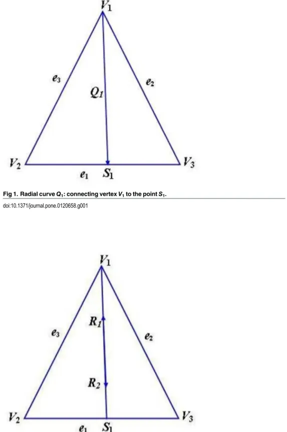
curveQ1connecting vertexV1to the pointsS1on the opposite edgese1is defined as (Fig 1):

Q1¼

Q1n

Q1d

; ð7Þ

where

Q1n ¼ ð1 sinlÞ

3

F1a1þsinlð1 sinlÞ 2

b1F1þ

2R1a1

p

þ cosl^ð1 cos^lÞ2

g1FðS1Þ

2d₁R2

p

þ ð1 cos^lÞ3

d1FðS1Þ;

Q1d ¼ a1ð1 sinlÞ 3

þb₁sinlð1 sinlÞ2þg₁cos^lð1 cos^lÞ2þd₁ð1 cosl^Þ3:

such that

l¼p

2ð1 uÞ; ^

l¼1 l:

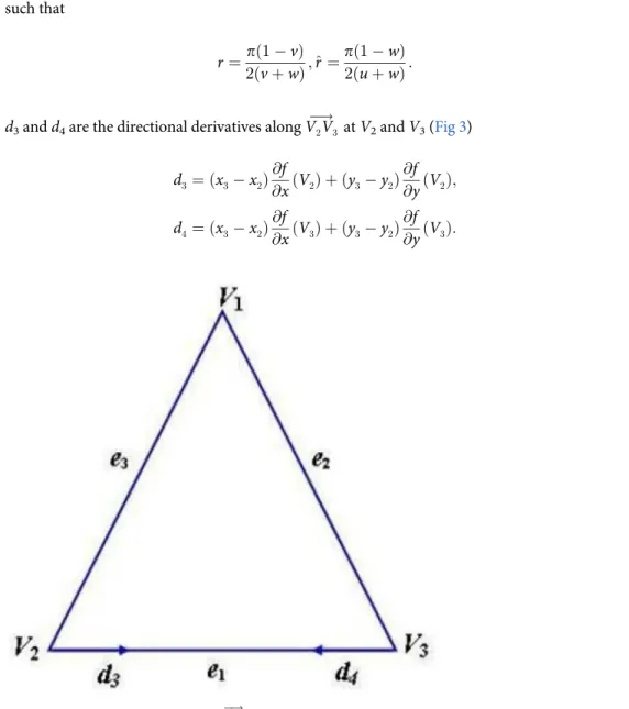
R1andR2are the directional derivatives atV1andS1(Fig 2) defined as

R1 ¼ ðxs1 x1Þ

@f

@xðV1Þ þ ðys1 y1Þ

@f

@yðV1Þ;

R2 ¼ ðxs1 x1Þ

@f

@xðS1Þ þ ðys1 y1Þ

@f

@yðS1Þ:

andF(S1) is the boundary curve along the edgee1evaluated from the following expression

FðS1Þ ¼

F1n

F1d

Fig 2. Directional derivatives alongS₁!V₁.

doi:10.1371/journal.pone.0120658.g002

Fig 1. Radial curveQ₁: connecting vertexV₁to the pointS₁.

where

F1n ¼ ð1 sinrÞ

3

F2a4þsinrð1 sinrÞ 2

b₄F2þ

2d3a4

p

þ cos^rð1 cos^rÞ2 g4F3

2d4d4

p

þ ð1 cos^rÞ3d4F3;

F1d ¼ a4ð1 sinrÞ 3

þb4sinrð1 sinrÞ 2

þg4cos^rð1 cos^rÞ 2

þd4ð1 cos^rÞ 3

:

such that

r¼pð1 vÞ

2ðvþwÞ;^r ¼

pð1 wÞ

2ðuþwÞ:

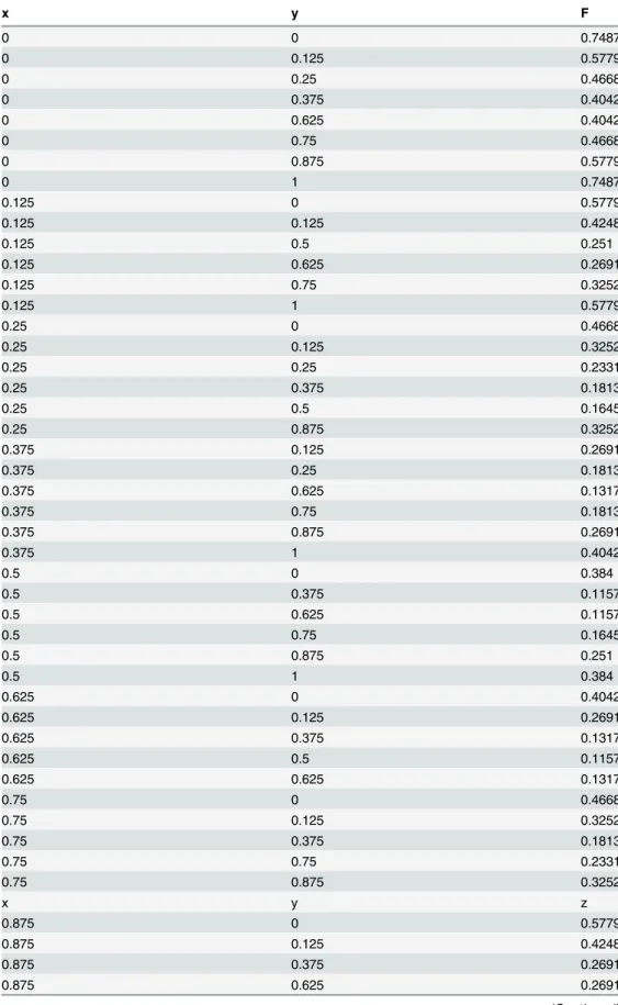
d3andd4are the directional derivatives alongV2V3

!

atV2andV3(Fig 3)

d3¼ ðx3 x2Þ @f

@xðV2Þ þ ðy3 y2Þ @f

@yðV2Þ;

d4¼ ðx3 x2Þ @f

@xðV3Þ þ ðy3 y2Þ @f

@yðV3Þ:

Fig 3. Directional derivatives alongV₂!V_3.

FromEq 7,Q1>0 if

Q1n>0andQ1d >0:

Now,Q1n>0 if

a1 >0;d1>0;

b1>

2R1a1

pF1 ;

g₁> 2R2d1

pFðS1Þ ;

FðS1Þ>0 :

ð8Þ

From Theorem 2.1,F(S1)>0 if

b4>

2a4d3

pF2 ;g4>

2d4d4

pF3

: ð9Þ

Now,Q1d>0 if

a₁ >0;b₁>0;g₁>0and d₁ >0:

Likewise, radial curveQ2connecting vertexV2to the pointsS2on the opposite edgese2is

de-fined as

Q2 ¼

Q2n

Q2d

; ð10Þ

where

Q2n ¼ ð1 sinmÞ

3

F2a2þ sinmð1 sinmÞ 2

b2F2þ

2R3a2

p

þ cosm^ð1 cosm^Þ2 g2FðS2Þ

2d₂R4

p

þ ð1 cosm^Þ3d2FðS2Þ;

Q2d ¼ a2ð1 sinmÞ 3

þb₂sinmð1 sinmÞ2þg₂cosm^ð1 cos^mÞ2þd₂ð1 cosm^Þ3:

such that

m¼p

2ð1 vÞ;m^¼1 m: ð11Þ

R3andR4are the directional derivatives atV2andS2

R3 ¼ ðxs2 x2Þ

@f

@xðV2Þ þ ðys2 y2Þ

@f

@yðV2Þ

R4 ¼ ðxs2 x2Þ

@f

@xðS2Þ þ ðys2 y2Þ

@f

@yðS2Þ

andF(S2) is the boundary curve along the edgee2to be evaluated from the following

expres-sion

FðS2Þ ¼

F2n

F2d

where

F2n ¼ ð1 sinsÞ

3

F3a5þsinrð1 sinrÞ 2

b₅F3þ

2d5a5

p

þ cosrð1 cosrÞ2 g₅F1

2d5d6

p

þ ð1 cosrÞ3d₅F1;

F2d ¼ a5ð1 sinrÞ 3

þb5sinrð1 sinrÞ 2

þg5cosrð1 cosrÞ 2

þd5ð1 cosrÞ 3

:

d5andd6are the directional derivatives alongV1V3

!

atV1andV3

d5 ¼ ðx1 x3Þ @f

@xðV3Þ þ ðy1 y3Þ @f

@yðV3Þ;

d6 ¼ ðx3 x2Þ @f

@xðV1Þ þ ðy3 y2Þ @f

@yðV1Þ:

FromEq 10,Q2>0 if

Q2n>0andQ2d >0:

Now,Q2n>0 if

a2>0; d2>0;

b2>

2R3a2

pF2 ;

g2 >

2R4d2

pFðS2Þ ;

FðS2Þ>0 :

ð12Þ

From Theorem 2.1,F(S2)>0 if

b5 >

2a5d5

pF3 ;g5 >

2d5d6

pF1

: ð13Þ

Now,Q2d>0 if

a2>0;b2 >0;g2 >0andd2>0:

and the radial curveQ3connecting vertexV3to the pointS3on the opposite edgee3is defined

as

Q3 ¼

Q3n

Q3d

; ð14Þ

where

Q3n ¼ ð1 sinnÞ

3

F3a3þsinnð1 sinnÞ 2

b₃F3þ

2R5a3

p

þ cosnð1 cosnÞ2

g3FðS3Þ

2d3R6

p

þ ð1 cosnÞ3

d3FðS3Þ;

Q3d ¼ a3ð1 sinnÞ 3

þb3sinnð1 sinnÞ 2

þg3cosnð1 cosnÞ 2

þd3ð1 cosnÞ 3

whereR5andR6are the directional derivatives atV3andS3defined as

R5 ¼ ðxs3 x3Þ

@f

@xðV3Þ þ ðys3 y3Þ

@f

@yðV3Þ

R6 ¼ ðxs3 x3Þ

@f

@xðS3Þ þ ðys3 y3Þ

@f

@yðS3Þ

andF(S3) is the boundary curve along the edgee3to be evaluated from the following

expres-sion

FðS3Þ ¼

F3n

F3d

;

where

F3n ¼ ð1 sintÞ

3

F1a6þ sintð1 sintÞ 2

b6F1þ

2d1a6

p

þ costð1 costÞ2 g₆F2

2d₆d2

p

þ ð1 costÞ3d₆F2;

F3d ¼ a6ð1 sintÞ 3

þb₆sintð1 sintÞ2þg₆costð1 costÞ2þd₆ð1 costÞ3:

d1andd2are the directional derivatives alongV1V2

!

atV1andV2

d5 ¼ ðx2 x1Þ @f

@xðV1Þ þ ðy2 y1Þ @f

@yðV1Þ;

d6 ¼ ðx2 x1Þ @f

@xðV2Þ þ ðy2 y1Þ @f

@yðV2Þ:

FromEq 14,Q3>0 if

Q3n>0 and Q3d >0:

Now,Q3n>0 if

a3>0; d2>0;

b3>

2R5a3

pF3 ;

g3 >

2R6d3

pFðS3Þ ;

FðS3Þ>0 :

ð15Þ

From Theorem 2.1,F(S3)>0 if

b₆ > 2a6d1

pF1

;g₆ >2d6d2

pF2

: ð16Þ

Now,Q3d>0 if

a₃ >0;b₃>0;g₃>0and d₃ >0:

Theorem 4.1The C1triangular pactch P inEq (4)is positive if the following conditions are attained.

a₁>0;a₂>0;a₃ >0;a₄>0;a₅>0;a₆ >0;

d1>0;d2>0;d3 >0;d4>0;d5>0;d6 >0;

b₁> max 0; 2R1a1

pF1

;g₁ > max 0;2R2d1

pFðS1Þ

;

b2> max 0;

2R3a2

pF2

;g2 > max 0;

2R4d2

pFðS2Þ

;

b3> max 0;

2R5a3

pF3

;g3 > max 0;

2R6d3

pFðS3Þ

;

b4> max 0;

2a₄d3

pF2

;g4> max 0;

2d₄d4

pF3

;

b₅> max 0; 2a5d5

pF3

;g₅> max 0;2d5d6

pF1

;

b₆> max 0; 2a6d1

pF1

;g₆> max 0;2d6d2

pF2

:

The above constraints can be rearranged as

b1>l1þmax 0;

2R1a1

pF1

;g1 >m1þmax 0;

2R2d1

pFðS1Þ

;l1;m1>0;

b2>l2þmax 0;

2R3a2

pF2

;g2 >m2þmax 0;

2R4d2

pFðS2Þ

;l2;m2>0;

b₃>l3þmax 0;

2R5a3

pF3

;g₃ >m3þmax 0;

2R6d3

pFðS3Þ

;l3;m3>0;

b₄>l4þmax 0;

2a4d3

pF2

;g₄>m4þmax 0;

2d4d4

pF3

;l4;m4>0;

b5>l5þmax 0;

2a5d5

pF3

;g5>m5þmax 0;

2d5d6

pF1

;l5;m5>0;

b6>l6þmax 0;

2a6d1

pF1

;g6>m6þmax 0;

2d6d2

pF2

;l6;m6>0:

5. Numerical Examples

This section illustrates the positivity preserving scheme for scattered data devised in Section 4.3.

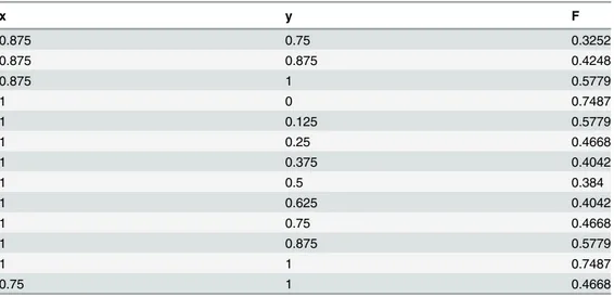
Example 5.1Positive scattered data is taken inTable 1.Fig 4represents corresponding delau-nay triangulations. The data is interpolated first byEq (4)for arbitrary values of free parame-ters,α1= 4.1,α2= 3;α3= 2.5,α4= 1.6,α5= 2.7,α6= 2.8,β1= 3.8,β2= 2.4,β3= 4.2,β4= 2.5,β5

Table 1. A Positive scattered data set I.

x y F

0 0 0.7487

0 0.125 0.5779

0 0.25 0.4668

0 0.375 0.4042

0 0.625 0.4042

0 0.75 0.4668

0 0.875 0.5779

0 1 0.7487

0.125 0 0.5779

0.125 0.125 0.4248

0.125 0.5 0.251

0.125 0.625 0.2691

0.125 0.75 0.3252

0.125 1 0.5779

0.25 0 0.4668

0.25 0.125 0.3252

0.25 0.25 0.2331

0.25 0.375 0.1813

0.25 0.5 0.1645

0.25 0.875 0.3252

0.375 0.125 0.2691

0.375 0.25 0.1813

0.375 0.625 0.1317

0.375 0.75 0.1813

0.375 0.875 0.2691

0.375 1 0.4042

0.5 0 0.384

0.5 0.375 0.1157

0.5 0.625 0.1157

0.5 0.75 0.1645

0.5 0.875 0.251

0.5 1 0.384

0.625 0 0.4042

0.625 0.125 0.2691

0.625 0.375 0.1317

0.625 0.5 0.1157

0.625 0.625 0.1317

0.75 0 0.4668

0.75 0.125 0.3252

0.75 0.375 0.1813

0.75 0.75 0.2331

0.75 0.875 0.3252

x y z

0.875 0 0.5779

0.875 0.125 0.4248

0.875 0.375 0.2691

0.875 0.625 0.2691

Table 1. (Continued₎

x y F

0.875 0.75 0.3252

0.875 0.875 0.4248

0.875 1 0.5779

1 0 0.7487

1 0.125 0.5779

1 0.25 0.4668

1 0.375 0.4042

1 0.5 0.384

1 0.625 0.4042

1 0.75 0.4668

1 0.875 0.5779

1 1 0.7487

0.75 1 0.4668

doi:10.1371/journal.pone.0120658.t001

Fig 4. Delaunay triangulation of positive data inTable 1.

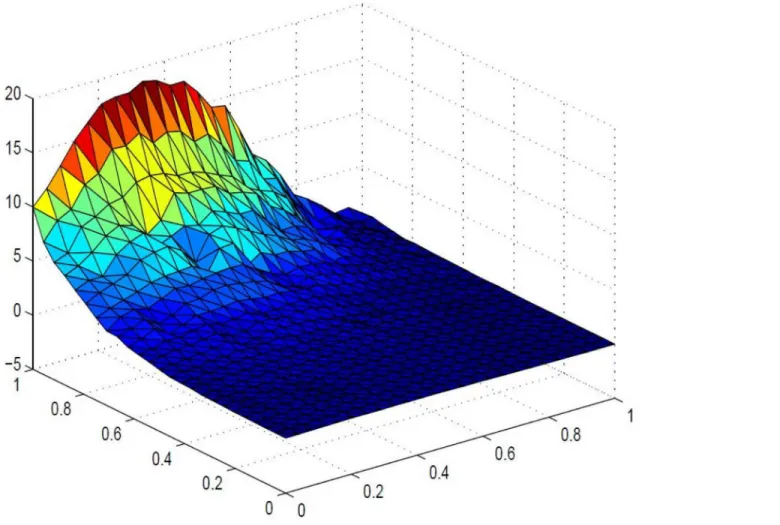
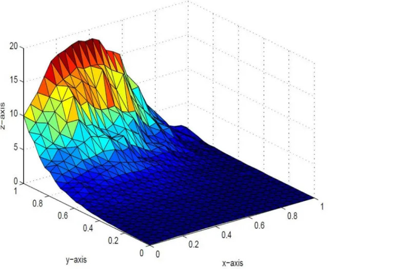
of positivity of data could no be held in visual model. This detriment is removed inFigs6,7and 8by implementing positivity preserving conditions summarized in Theorem 4.1. It is worth men-tioning here that parametersα_iandδ_ifor i= 1,2,. . .,6are left free to refine the shape according to user’s requirement. The effect of free parameters are shown inFigs6,7and8. Figs6and7are constructed against the parameter choiceα₁= 12,α₂= 0.4,α₃= 13,α₄= 0.22,α₅= 12,α₆= 0.33,

δ1= 13,δ2= 0.3,δ3= 14,δ4= 0.3,δ5= 15,δ6= 12 andα1= 0.1,α2= 1.0,α3= 0.5,α4= 1.6, α₅= 0.7,α₆= 0.8,δ₁= 0.8,δ₂= 0.4,δ₃= 1.2,δ₄= 1.5,δ₅= 1.5,δ₆= 1.0respectively, which lacks smoothness. A smooth visibly pleasant representation is obtained inFig 8by settingα1= 1.0, α₂= 1.0,α₃= 0.5,α₄= 0.6,α₅= 0.7,α₆= 0.8,δ₁= 0.8,δ₂= 0.4,δ₃= 1.2,δ₄= 0.5,δ₅= 1.0,

δ6= 1.0

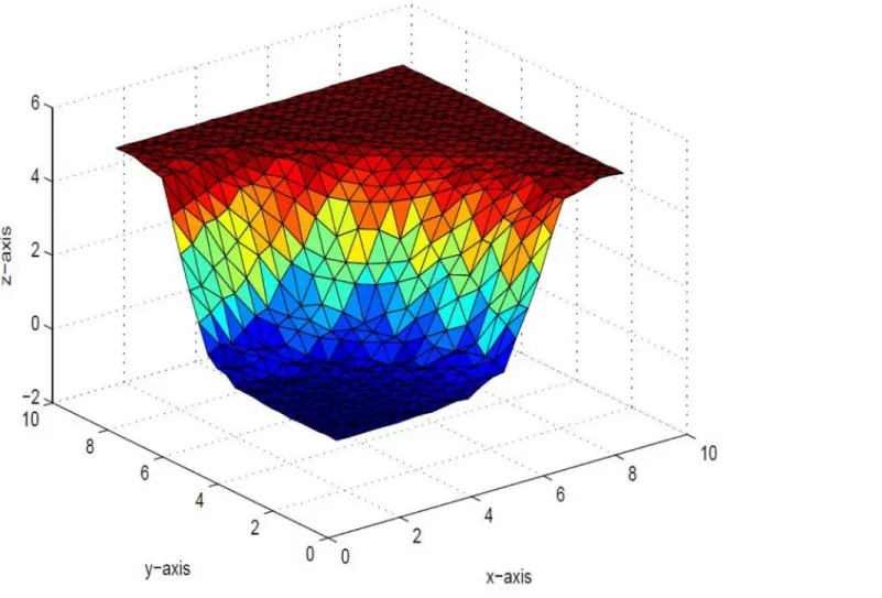
Example 5.2A Positive scattered data set is displayed inTable 2.Delauny triangulation is il-lustrated inFig 9and the corresponding surface inFig 10is obtained by interpolating the data Fig 5. Rational cubic trigonometric surface of the positive data inTable 1.

for arbitrary values of free parameters,α₁= 4.1,α₂= 3;α₃= 2.0,α₄= 1.5,α₅= 2.7,α₆= 2.5,β₁= 3.5,β2= 2.3,β3= 3.2,β4= 2.2,β5= 1.0,β6= 4.5,γ1= 1.4,γ2= 5.5,γ3= 1.5,γ4= 2.2,γ5= 1.5,γ1

= 2.5,δ₁= 0.5,δ₂= 3.1,δ₃= 3.5,δ₄= 0.4,δ₅= 2,δ₆= 1.2,in description ofEq (4).It is evident fromFig 10that the positivity of data could not be conserved in visual model. This impediment is removed inFigs11,12andFig 13by implementing positivity preserving constraints on parame-tersβi,γifor i= 1,2,. . .,6,summarized in Theorem 4.1. Here, it is noteworthy that parametersαi

andδ_ifor i= 1,2,. . .,6are set free to refine the shape as required by the user. The effect of free pa-rameters are shown inFigs11,12and13. Figs11and12are constructed against the parameter choiceα₁= 2.0,α₂= 0.1,α₃= 0.5,α₄= 0.5,α₅= 1.0,α₆= 0.63,δ₁= 1.0,δ₂= 0.33,δ₃= 0.5,δ₄= 0.4,δ5= 1.0,δ6= 0.3andα1= 2.2,α2= 1.1,α3= 2.5,α4= 1.5,α5= 1.0,α6= 1.0,δ1= 1.0,δ2=

1.0,δ₃= 1.5,δ₄= 1.4,δ₅= 1.0,δ₆= 0.3respectively, which lacks smoothness. A smooth visibly pleasant representation is obtained inFig 13by settingα1= 2.0,α2= 0.4,α3= 0.5,α4= 0.5,α5=

1.0,α₆= 0.63,δ₁= 0.3,δ₂= 0.33,δ₃= 0.5,δ₄= 0.3,δ₅= 0.5,δ₆= 0.2. Fig 6. Positive surface generated from Theorem 4.1 of the positive data inTable 1.

Conclusion

In this study, positivity preserving algorithm for scattered data arranged over a triangular do-main, is established. The rational trigonometric cubic function [13] with four free parameters is used for the interpolation along each boundary and radial curve. Nielson side vertex has been applied to construct the interpolating surface. Constraints on half of the parameters are obtained to guarantee the positive shape of data while half are set free for users modification. The proposed algorithm, surpasses many prevailing approaches in literature. In [10], authors Fig 7. Positive surface generated from Theorem 4.1 of the positive data inTable 1.

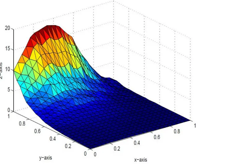
Fig 8. Positive surface generated from Theorem 4.1 of the positive data inTable 1.

doi:10.1371/journal.pone.0120658.g008

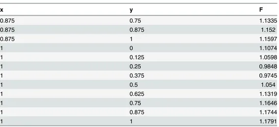
Table 2. A Positive scattered data set II.

x y F

0 0 0.4486

0 0.125 0.3616

0 0.25 0.4692

0 0.375 0.6827

0 0.5 0.786

0 0.625 0.836

0 0.75 0.8765

0 0.875 0.9125

0 1 0.9447

0.125 0 0.3369

0.125 0.125 0.0001

0.125 0.375 0.6256

0.125 0.625 0.8621

Table 2. (Continued₎

x y F

0.125 0.875 0.9334

0.125 1 0.9634

0.25 0 0.4529

0.25 0.125 0.1767

0.25 0.25 0.3217

0.25 0.375 0.7005

0.25 0.5 0.8555

0.25 0.625 0.9327

0.25 0.75 0.9775

0.25 0.875 0.9686

0.25 1 0.9926

0.375 0 0.696

0.375 0.375 0.8363

0.375 0.625 1.2176

0.375 0.875 1.028

0.375 1 1.0284

0.5 0 0.8329

0.5 0.125 0.8315

0.5 0.25 0.821

0.5 0.375 0.8498

0.5 0.5 0.925

0.5 0.625 1.0925

0.5 0.75 1.1688

0.5 0.875 1.0568

0.5 1 1.0662

0.625 0 0.9049

0.625 0.125 0.8376

0.625 0.375 0.7163

0.625 0.5 0.8608

0.625 0.75 1.0671

0.625 0.875 1.0883

0.625 1 1.1023

0.75 0 0.9639

0.75 0.125 0.8326

0.75 0.25 0.6283

0.75 0.375 0.5976

0.75 0.5 0.8075

0.75 0.625 1.0136

0.75 0.75 1.0989

0.75 0.875 1.1231

0.75 1 1.134

0.875 0 1.0355

0.875 0.125 0.922

0.875 0.25 0.7477

0.875 0.375 0.7193

0.875 0.5 0.893

0.875 0.625 1.0638

Table 2. (Continued₎

x y F

0.875 0.75 1.1335

0.875 0.875 1.152

0.875 1 1.1597

1 0 1.1074

1 0.125 1.0598

1 0.25 0.9848

1 0.375 0.9745

1 0.5 1.054

1 0.625 1.1319

1 0.75 1.1646

1 0.875 1.1744

1 1 1.1791

doi:10.1371/journal.pone.0120658.t002

Fig 9. Delaunay triangulation of positive data inTable 2.

utilized a cubic function with one free parameter to retain the positive shape of data. Positive surface was obtained by drawing data dependent constraints on this free parameter, and, hence the scheme did not offer refinement in the shape. The scheme suggested in this paper does not suffer this detriment. The developed algorithm is local and can be applied to data with or with-out derivatives. Moreover, shape preserving algorithms play an instrumental role in many areas of visualization such as geometric modelling, robot trajectories, evolution game theory, prisoner’s dilemma game [16], [17], [18], meshless method and inverse kinemaics etc. Fig 10. Rational cubic trigonometric surface of the positive data.

Author Contributions

Conceived and designed the experiments: FI MZH AB. Performed the experiments: FI MZH AB. Analyzed the data: FI MZH AB. Contributed reagents/materials/analysis tools: FI MZH AB. Wrote the paper: FI MZH AB.

References

1. Sarfraz M, Hussain MZ, Arfan M. Positivty preserving scattered data interpolation scheme using the side vertex method. Applied Mathematics and Computation. 2012; 218(15):7898–7910. doi:10.1016/j. amc.2012.01.072

2. Franke R, Nielson GM. Smooth interpolation of larger sets of scattered data. International Journal of Numerical Methods in Engineering. 1980; 15:1691–1704. doi:10.1002/nme.1620151110

3. Kraus V, Dehmer M, Emmert-Streib F. Probabilistic inequalities for evaluating structural network mea-sures. Information Sciences. 2014; 288:220–245. doi:10.1016/j.ins.2014.07.018

4. Dehmer M, Emmert-Streib F, Shi Y. Interrelations of graph distance measures based on topological in-dices. PLoS ONE. 2014; 9.

5. Cao S, Dehmer M, Shi Y. Extremality of degree-based graph entropies. Information Sciences. 2014; 278:22–33. doi:10.1016/j.ins.2014.03.133

6. Gupta MK, Niyogi R, Misra M. A 2D Graphical Representation of Protein Sequence and Their Similarity Analysis with Probabilistic Method. MATCH Communications in Mathematical and in Computer Chem-istry. 2014; 72:519–532.

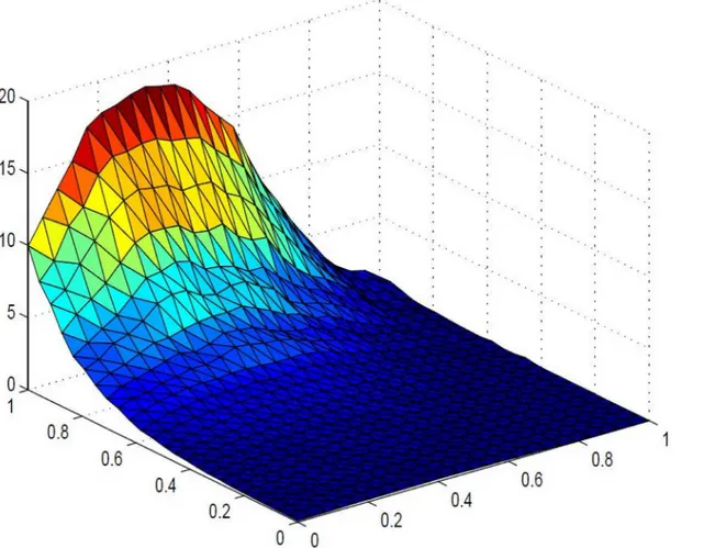
Fig 13. Positive surface generated from Theorem 4.1.

7. Amidor I. Scattered data interpolation methods for electronic imaging systems:survey. Journal of Elec-tronic Imaging. 2002; 11(2):157–176. doi:10.1117/1.1455013

8. Dougherty RL, Edelman Z, Hyman JM. Non-negativity, monotonicity or convexity preserving cubic and quintic Hermite interpolation. Mathematics of Computation. 1989; 52(186):471–494. doi:10.1090/ S0025-5718-1989-0962209-1

9. Piah ARM, Goodman TNT, Unsworth K. Positivity preserving scattered data interpolation. In: Martin R, Bez H, Sabin M, editors. Proceeding of Mathematics of Surfaces, Lecture Notes in Computer Sci-ence,3604. New York: Springer-Verlag Berlin Heidelberg; 2005. p. 336–349.

10. Hussain MZ, Hussain M. Shape preserving scattered data interpolation. European Journal of Scientific Research. 2009; 25(1):151–164.

11. Hermann M, Mulansky B, Schmidt JW. Scattered data interpolation subject to piecewise quadratic range restriction. Journal of Computational and Applied Mathematics. 1996; 73:209–223. doi:10.1016/ 0377-0427(96)00044-1

12. Hussain MZ, Hussain M.C1positivity preserving scattered dat interpolation using Bernstein Bezier tri-angular patch. Journal of Applied Mathematics and Computing. 2011; 35:281–293. doi:10.1007/ s12190-009-0356-0

13. Ibraheem F, Hussain M, Hussain MZ, Bhatti AA. Data visualizaation using Trigonometric function. Jour-nal of Applied Mathematics. 2012; 2012:1–19. doi:10.1155/2012/247120

14. Nielson GM. The side-vertex method for interpolation in triangles. Journal of Approximatio Theory. 1979; 25:316–336.

15. Goodman TNT, Said HB, Chang LHT. Local derivative estimation for scattered data interpolation. Ap-plied Mathematics and Computation. 1995; 68:41–50. doi:10.1016/0096-3003(94)00086-J

16. Davidson KR. The Evolution of Cooperation. Newyork: Basic Books; 2006.

17. Ma ZQ, Xia CY, Sun SW, Wang L, Wang HB, Wang J. Heterogeneous link weight promotes the cooper-ation in spatial prisoner’s dilemma. International Journal of Modern Physics C. 2011; 22:1257–1258. doi:10.1142/S0129183111016877