SRef-ID: 1684-9981/nhess/2006-6-115 European Geosciences Union
© 2006 Author(s). This work is licensed under a Creative Commons License.
and Earth
System Sciences
Landslide hazard assessment in the Collazzone area, Umbria,
Central Italy
F. Guzzetti, M. Galli, P. Reichenbach, F. Ardizzone, and M. Cardinali
IRPI CNR, via Madonna Alta 126, 06128 Perugia, Italy
Received: 2 November 2005 – Revised: 20 December 2005 – Accepted: 20 December 2005 – Published: 31 January 2006
Abstract. We present the results of the application of a
re-cently proposed model to determine landslide hazard. The model predicts where landslides will occur, how frequently they will occur, and how large they will be in a given area. For the Collazzone area, in the central Italian Apennines, we prepared a multi-temporal inventory map through the in-terpretation of multiple sets of aerial photographs taken be-tween 1941 and 1997 and field surveys conducted in the pe-riod between 1998 and 2004. We then partitioned the 79 square kilometres study area into 894 slope units, and ob-tained the probability of spatial occurrence of landslides by discriminant analysis of thematic variables, including mor-phology, lithology, structure and land use. For each slope unit, we computed the expected landslide recurrence by di-viding the total number of landslide events inventoried in the terrain unit by the time span of the investigated period. Assuming landslide recurrence was constant, and adopting a Poisson probability model, we determined the exceedance probability of having one or more landslides in each slope unit, for different periods. We obtained the probability of landslide size, a proxy for landslide magnitude, by analysing the frequency-area statistics of landslides, obtained from the multi-temporal inventory map. Lastly, assuming indepen-dence, we determined landslide hazard for each slope unit as the joint probability of landslide size, of landslide tempo-ral occurrence, and of landslide spatial occurrence.
1 Introduction
Prediction of landslide hazard involves determining “where” landslides are expected, “when” or how frequently they will occur, and the “magnitude” of the landslides, i.e., how large or destructive the slope failures will be. Several methods have been proposed to evaluate where landslides are ex-pected (e.g., Carrara, 1983; Carrara et al., 1991, 1995; van
Correspondence to: F. Guzzetti
Westen, 1994; Soeters and van Westen, 1996; Chung and Fabbri, 1999; Guzzetti et al., 1999, and references herein). To predict the location of future landslides, these meth-ods use statistical classification techniques and exploit the known, inferred, or expected relationship between past land-slides in an area and a set of geo-environmental thematic variables in the same area. Attempts have been made to pre-dict “when” landslides will occur by determining the proba-bility of landslide occurrence in a given period (e.g., Keaton et al., 1988; Lips and Wieczorek, 1990; Coe et al., 2000; Crovelli, 2000; Guzzetti et al., 2003). Most commonly, the temporal probability of landslide occurrence is obtained from catalogues of historical landslide events or multi-temporal landslide inventory maps. No single measure of landslide “magnitude” exists (Hungr, 1997). For some landslide types, landslide area is a reasonable proxy for landslide magnitude. The frequency-area statistics of landslides can be obtained from accurate landslide inventory maps (Stark and Hovius, 2001; Guzzetti et al., 2002; Malamud et al., 2004), and this information can be used as a proxy for the distribution of landslide magnitude in an area.
In this paper, we apply a recently proposed model for the probabilistic assessment of landslide hazard (Guzzetti et al., 2005). The model exploits information obtained from a multi-temporal inventory map to predict where landslides will occur, how frequently they will occur, and how large they will be. We test the model in the Collazzone area, in the central Apennines of Italy, and we discuss the results ob-tained.
2 The study area
Fig. 1. Location map. (A) Shaded relief image of the Umbria Re-gion. (B) Shaded relief image showing morphology in the Col-lazzone area. (C) Lithological map for the ColCol-lazzone area: (1) Alluvial deposits, Holocene in age, (2) Continental deposits, Plio-Pleistocene in age, (3) Travertine, Plio-Pleistocene in age, (4) Layered sandstone and marl, Miocene in age, (5) Thinly layered limestone, Lias to Oligocene in age. (D) Image showing a three-dimensional view of the study area seen from West.
Rio creeks. Landscape is predominantly hilly, and lithology and the attitude of bedding planes control the morphology of the slopes. Valleys oriented N–S are shorter, asymmetri-cal, and parallel to the main direction of the bedding plains, whereas valleys oriented E–W are longer, symmetrical, and mostly perpendicular to the direction of the bedding planes. In the area crop out sedimentary rocks, including (Fig. 1c): (i) recent fluvial deposits, chiefly along the main valley bot-toms, (ii) continental gravel, sand and clay, Plio-Pleistocene in age, (iii) travertine deposits, Pleistocene in age, (iv) lay-ered sandstone and marl in various percentages, Miocene in age, and (v) thinly layered limestone, Lias to Oligocene in age (Conti et al., 1977; Servizio Geologico Nazionale, 1980; Cencetti, 1990; Barchi et al., 1991). Soils in the area range in thickness from a few decimetres to more than one meter, they have a fine or medium texture, and exhibit a xenic mois-ture regime, typical of the Mediterranean climate. Annual rainfall averages 885 mm, and is most abundant in the period from September to December. Landslides are abundant in the area, and range in type and volume from very old and partly dismantled large deep-seated slides to shallow slides and flows).
3 Probabilistic model of landslide hazard
We have recently proposed a probabilistic model for the as-sessment of landslide hazard (Guzzetti et al., 2005). The model is based on the definition given by Guzzetti et al. (1999), who defined landslide hazard as “the probability
of occurrence within a specified period and within a given area of a potentially damaging landslide of a given magni-tude”. Guzzetti et al. (1999) amended the definition of
land-slide hazard given by Varnes and the IAEG Commission on Landslides and other Mass-Movements (1984) to include the magnitude (i.e., the size, intensity or destructiveness) of the expected landslide event (Einstein, 1988; Canuti and Casagli, 1994; Hungr, 1997; Guzzetti et al., 2005).
In mathematical terms, the adopted definition of landslide hazard can be written:
HL=P[AL≥aL in a time interval t, given
{morphology, lithology, structure, land use,. . .}](1) where,ALis the area of a landslide greater or equal than a minimum size,aL,measured e.g., in square meters. For any given area, proposition (1) can be written as:
HL=P (AL)×P (NL)×P (S) (2)
that expresses landslide hazardHLas the conditional prob-ability of landslide size P (AL), of landslide occurrence in an established periodP (NL), and of landslide spatial occur-renceP (S), given the local environmental setting.
Equation (2) assumes independence of the three individ-ual probabilities, i.e., of the three components of landslide hazard. From a geomorphological point of view, this as-sumption is severe and may not hold, always and everywhere (Guzzetti et al., 2005). In many areas we expect slope fail-ures to be more frequent (time component) where landslides are more abundant and landslide area is large (spatial com-ponent). However, given the lack of understanding of the landslide phenomena, independence is an acceptable approx-imation that makes the problem mathematically tractable and easier to work with. In the discussion, we will examine the validity of this assumption for the study area.
In a previous work, we have proposed a method to obtain all the relevant information needed to apply the probabilis-tic model (Guzzetti et al., 2005). The method is based on the systematic interpretation of multiple sets of aerial pho-tographs of different dates, aided by historical investigations and field surveys, to obtain a detailed multi-temporal land-slide inventory map. The multi-temporal inventory is then exploited to: (i) obtain the spatial probability of landslide oc-currence, given the local environmental setting, (ii) estimate the temporal probability of landslides, from the empirical re-currence of slope failures, and (iii) determine the probabil-ity of landslide size (area), considered a proxy for landslide magnitude.
In the following, we first describe how we have collected the landslide information in the Collazzone area. Next, we demonstrate how the landslide information can be used to determine landslide hazard. Lastly, we discuss the problems encountered and the limitations of the obtained hazard as-sessment.
4 Multi-temporal landslide inventory map
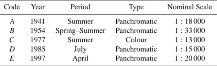
Table 1. Collazzone study area, central Umbria. Aerial pho-tographs used to prepare the multi-temporal landslide inventory map shown in Fig. 2.
Code Year Period Type Nominal Scale
A 1941 Summer Panchromatic 1:18 000
B 1954 Spring–Summer Panchromatic 1:33 000
C 1977 Summer Colour 1:13 000
D 1985 July Panchromatic 1:15 000
E 1997 April Panchromatic 1:20 000
the interpretation of multiple sets of aerial photographs and detailed geological and geomorphological field mapping (Fig. 2). To prepare the landslide inventory, we used five sets of aerial photographs ranging in scale from 1:13 000 to 1:33 000 and covering unsystematically the period from 1941 to 1997 (Table 1). A team of two geomorphologists car-ried out the interpretation of the aerial photographs in the 5-month period from July to November 2002. The interpreters analyzed each pair of aerial photographs using a mirror stere-oscope (4×magnification) and a continue-zoom stereoscope (3×to 20×magnification). Both stereoscopes allowed the interpreters to map contemporaneously on the same stereo pair. The interpreters used all morphological, geological and landslide information available from published maps, and previous works carried out in the same area (e.g., Servizio Geologico Nazionale, 1980, Guzzetti and Cardinali, 1989, 1990; Antonini et al., 20021). Care was taken in identifying areas where morphology had changed in response to individ-ual or multiple landslides, and to avoid interpretation errors due to land use modifications or to different views provided by aerial photographs taken at different dates.
The inventory map obtained from the analysis of the aerial photographs was successively updated to cover the period from 1998 to 2004 through field surveys conducted chiefly following periods of prolonged rainfall. Due to lack of aerial photographs taken after recent rainfall events, the rainfall-induced landslides were mapped directly in the field at 1:10 000 scale. Colour photographs taken in the field with a handheld digital camera were used to aid the mapping and the classification of the landslides locally.
Adopting an established procedure in Umbria (Cardinali et al., 2002b; Reichenbach et al., 2005), in the multi-temporal 1Antonini, G., Ardizzone, F., Cacciano, M., Cardinali, M.,
Castellani, M., Galli, M., Guzzetti, F., Reichenbach, P., and Sal-vati, P.: Rapporto Conclusivo Protocollo d’Intesa fra la Regione dell’Umbria, Direzione Politiche Territoriali Ambiente e Infrastrut-ture, ed il CNR-IRPI di Perugia per l’acquisizione di nuove infor-mazioni sui fenomeni franosi nella regione dell’Umbria, la realiz-zazione di una nuova carta inventario dei movimenti franosi e dei siti colpiti da dissesto, l’individuazione e la perimetrazione delle aree a rischio da frana di particolare rilevanza, e l’aggiornamento delle stime sull’incidenza dei fenomeni di dissesto sul tessuto inse-diativo, infrastrutturale e produttivo regionale, (in Italian), Unpub-lished report, May 2002, 140 p., 2002.
F1 - F2 - F3
E1 - E2
D1 - D2
C1 - C2
B1 - B2
A2
A1
A0
Fig. 2. Multi-temporal landslide inventory map for the Collazone area. See Fig. 1 for location. Colours show landslides of different age, inferred from the date of the aerial photographs and of field surveys. A0, very old relict landslide; A1, landslides older than 1941; A2, active landslides in 1941; B1–B2, landslides in the period from 1941 to 1954; C1–C2, landslides in the period from 1954 to 1977; D1–D2, landslides in the period from 1977 to 1985; E1–E2, landslides in the period from 1985 to 1997; F1–F2–F3; landslides in the period from 1998 to 2004. See Table 2 and text for explanation.
age of a mass movement based on its appearance (McCalpin, 1984).
In each of the five sets of aerial photographs used to pre-pare the multi-temporal inventory, we separated landslides that appeared “fresh” on the aerial photographs, from the other landslides. We assigned the “fresh” slope failures the date (i.e., year) of the aerial photographs used to identify the landslides. The other slope failures (i.e., the “non-fresh” landslides) were attributed to the period between two suc-cessive sets of aerial photographs. The latter groups include landslides that exhibited morphological changes with respect to one or more of the older sets of aerial photographs. Land-slides mapped in the field after rainfall events in the period between 1998 and 2004 were attributed to three different dates, depending on the dates of the field surveys.
In the multi-temporal inventory (Fig. 2), very old (relict) landslides include deep-seated slope failures with an area AL>6.3×10⁴m2 (i.e., >6.3 ha) and an estimated volume VL>×106m3. These very old failures are present mostly in the head section of minor catchments, and are largely con-trolled by lithology, structure and the attitude of the bedding planes. In places, the very old landslides are covered by mul-tiple generations of younger landslides that have dismantled and cancelled the older landslides, making their recognition problematic. Old landslides include deep-seated and shal-low slope failures. The old, deep-seated failures are mostly rock/earth slides and complex earth slides – earth flows, extending from less than 1.0×10⁴m2 (1 ha) to more than 1.7×10⁵m2(17 ha). The morphology of the old landslides is similar to the morphology of the relict landslides, but the old failures are less affected by more recent slope failures. For this reason, recognition of old landslides is easier, in the field and from the aerial photographs. The old shallow landslides are mostly slide and flow, extending in area from less than 1.0×10³m2to 2.8×10⁴m2(2.8 ha). Recent landslides in the multi-temporal inventory consist chiefly of shallow failures that occurred in the 64-year period from 1941 to 2004, and include active slope failures at the date of the field surveys.
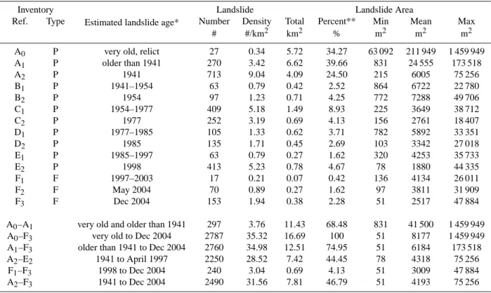
Table 2 summarizes statistics for the landslides in the multi-temporal inventory map. The entire inventory, cov-ering an undetermined period from pre-1941 to 2004 (A0– F3 in Table 2), shows 2787 landslides, including 27 very old and relict landslides, for a total mapped landslide area of 22.79 km2, which corresponds to a landslide density of 35.32 slope failures per square kilometre. Due to geographi-cal overlap of landslides of different periods, the total area af-fected by landslides is 16.69 km2, 21.16% of the studied area. Mapped landslides extend in size from 51 m2 to 1.45 km2, and the most represented (i.e., numerous, abundant) failures shown in the map have an area of about 8.15×10²m2. The inventory lists 2490 landslides (89.34%) for which the date or the period of occurrence was determined (A2–F3 in Ta-ble 2). These landslides have an average landslide size of 4.19×10³m2, for a total landslide area of 10.24 km2, cover-ing 7.81 km2(9.89% of the study area). These figures com-pare with 297 (10.66%) old and very old landslides whose age remained undetermined but was older than 1941. The old
and very old landslides have an average area of 4.15×10⁴m2, for a total landslide area of 12.34 km2, covering 11.43 km2 (14.48% of the study area). We attribute the largest abun-dance of landslides in the period from 1941 to 2004 to in-completeness of the multi-temporal map before 1941. We further attribute the large average landslide area of the very old and old landslides to amalgamation of smaller landslides into larger landslide areas. Very old and relict landslides may have also formed under different and more severe climatic or seismic conditions (Carrara et al., 1995).
5 Landslide hazard assessment
The Collazzone study area was first subdivided into slope units to determine landslide hazard. Slope units are terrain units bounded by drainage and divide lines (Carrara et al., 1991). Starting from a digital terrain model with a ground resolution of 10 m×10 m and a simplified representation of the main drainage lines, specific software partitioned the study area into 894 slope units. For each slope unit, the soft-ware computed 21 morphometric and hydrological parame-ters useful to explain the spatial distribution of landslides. To better represent the distinct limit between the hills and the Tiber River flood plain, avoiding the problem of slope units characterized by two distinct terrain types (e.g., sloping ter-rain and the flat terter-rain in the flood plain), a synthetic river channel was drawn in correspondence to the brake in slope. 5.1 Probability of landslide size
We ascertained the probability of landslide area, a proxy for landslide magnitude, for two datasets: (i) the entire multi-temporal inventory listing 2787 landslides (A0–F3 in Ta-ble 2), and (ii) the multi-temporal inventory covering the 64-year period from 1941 to 2004, listing 2490 landslides (A2–F3in Table 2). We obtained the area of the individual landslides in the GIS. Care was taken to calculate the ex-act size of each landslide, avoiding topological and graphical problems related to the presence of smaller landslides inside larger mass movements. For the deep-seated landslides, we merged the crown area and the deposit, and we used the total landslide area in the analysis.
Table 2. Collazzone study area, central Umbria. Landslide size and abundance. Figures obtained from the multi-temporal inventory map shown in Fig. 2. Inventory type: P, obtained from the systematic interpretation of stereoscopic aerial photographs; F, obtained through direct field mapping. See Table 1 for date of the aerial photographs used to complete the inventory. * Landslide age estimated from the date of the aerial photographs and the morphological appearance of the landslide. ** Percentage of landslide area with respect to the total area covered by landslides (A0–F3).
Inventory
Estimated landslide age*
Landslide Landslide Area
Ref. Type Number Density Total Percent** Min Mean Max
# #/km2 km2 % m2 m2 m2
A0 P very old, relict 27 0.34 5.72 34.27 63 092 211 949 1 459 949
A1 P older than 1941 270 3.42 6.62 39.66 831 24 555 173 518
A2 P 1941 713 9.04 4.09 24.50 215 6005 75 256
B1 P 1941–1954 63 0.79 0.42 2.52 864 6722 22 780
B2 P 1954 97 1.23 0.71 4.25 772 7288 49 706
C1 P 1954–1977 409 5.18 1.49 8.93 225 3649 38 712
C2 P 1977 252 3.19 0.69 4.13 156 2761 18 407
D1 P 1977–1985 105 1.33 0.62 3.71 782 5892 33 351
D2 P 1985 135 1.71 0.45 2.69 103 3342 27 018
E1 P 1985–1997 63 0.79 0.27 1.62 320 4253 35 733
E2 P 1998 413 5.23 0.78 4.67 78 1880 44 335
F1 F 1997–2003 17 0.21 0.07 0.42 136 4134 26 011
F2 F May 2004 70 0.89 0.27 1.62 97 3811 31 909
F3 F Dec 2004 153 1.94 0.38 2.28 51 2517 47 884
A0–A1 very old and older than 1941 297 3.76 11.43 68.48 831 41 500 1 459 949
A0–F3 very old to Dec 2004 2787 35.32 16.69 100 51 8177 1 459 949
A1–F3 older than 1941 to Dec 2004 2760 34.98 12.51 74.95 51 6184 173 518
A2–E2 1941 to April 1997 2250 28.52 7.42 44.45 78 4318 75 256
F1–F3 1998 to Dec 2004 240 3.04 0.69 4.13 51 3009 47 884
A2–F3 1941 to Dec 2004 2490 31.56 7.81 46.79 51 4193 75 256
Table 3. Collazzone study area, central Umbria. DP, double Pareto distribution (Stark and Hovius, 2001); IG, inverse Gamma distribution (Malamud et al., 2004).
Data set Period α Size of most abundant landslide (m
2)
DP IG DP IG
A0−F3 very old to Dec 2004 2.15 2.18 816 816
A2−F3 1941 to Dec 2004 2.48 2.54 881 1019
and the double Pareto distributions predict a significantly larger proportion of large (AL>1×10⁴m2) and very large (AL>1×10⁶m2)landslides, when compared to the estimates obtained from the reduced landslide dataset (A2–F3). We at-tribute the difference to the presence of a few very large and relict landslides in dataset A0–F3, which are not present in dataset A2–F3.
Figure 3II shows the probability of landslide size, i.e., the probability that a landslide will have an area smaller than a given size (left axis), or the probability that a landslide will have an area that exceeds a given size (right axis). Us-ing dataset A2–F3, the probability that a landslide exceeds 1×10³m2(i.e., slightly larger than the area of the most abun-dant landslide mapped in the multi-temporal inventory) is ∼0.80, and the probability that a landslide exceeds 1×10⁴m2
is∼0.10. We will use these statistics to ascertain landslide hazard.
5.2 Frequency of landslide occurrence
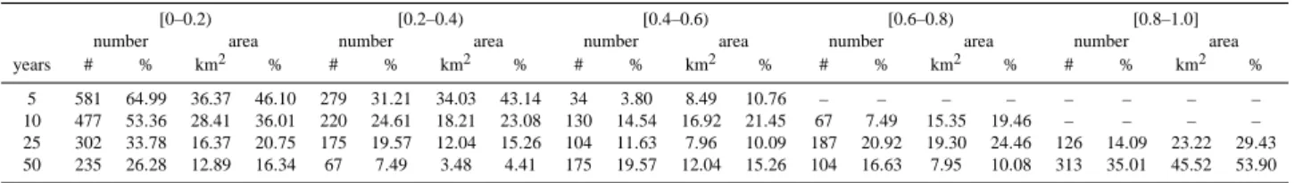
Table 4. Number and percentage of slope units, and total area and percentage of slope units, in five classes of the probability of temporal landslide occurrence (see Fig. 4). Square bracket indicates class limit is included; round bracket indicates class limit is not included. Temporal probability of landslide occurrence obtained exploiting the multi-temporal landslide inventory map (Fig. 2) and adopting a Poisson probability model. See text for explanation.
[0–0.2) [0.2–0.4) [0.4–0.6) [0.6–0.8) [0.8–1.0] number area number area number area number area number area years # % km2 % # % km2 % # % km2 % # % km2 % # % km2 %
5 581 64.99 36.37 46.10 279 31.21 34.03 43.14 34 3.80 8.49 10.76 – – – – – – – – 10 477 53.36 28.41 36.01 220 24.61 18.21 23.08 130 14.54 16.92 21.45 67 7.49 15.35 19.46 – – – – 25 302 33.78 16.37 20.75 175 19.57 12.04 15.26 104 11.63 7.96 10.09 187 20.92 19.30 24.46 126 14.09 23.22 29.43 50 235 26.28 12.89 16.34 67 7.49 3.48 4.41 175 19.57 12.04 15.26 104 16.63 7.95 10.08 313 35.01 45.52 53.90
Table 5. Variables entered into the seven discriminant models of landslide susceptibility (see Fig. 5). (A) Model obtained using landslides identified in the period A1; (B) model obtained using landslides in the period A1–A2; (C) model obtained using landslides in the period A1– B2; (D) model obtained using landslides in the period A1–C2; (E) model obtained using landslides in the period A1–D2; (F) model obtained using landslides in the period A1–E2; (G) model obtained using landslides in the period A1–F3. Standard discriminant function coefficients (SDFC) show the relative importance of each variable in the discriminant function. Coefficients shown in bold are strongly associated with the presence/absence of landslides. Positive coefficients are correlated to the absence of landslides. Negative coefficients are correlated to the presence of landslides.
Variable description Variable Model SDFC
A B C D E F G
Drainage channel order ORDER .162 .280 .181 .148 .146 .138
Drainage channel length LINK LEN –.425 –.198
Slope unit area SLO AREA –.358 –.269 –.255 –.264 –.247
Slope unit mean elevation ELV M –.673
Slope unit terrain elevation standard dev. ELV STD –.250 –.362 –.307 –.372 –.379 –.377
Slope unit mean terrain gradient SLO ANG –.385 –.695 –.675 –.392
Slope unit terrain gradient standard dev. ANG STD .310 .381 .308 .298 .355
Slope unit length SLO LEN –.230 –.210 –.213
Slope unit length standard deviation LEN STD .257
Slope unit terrain gradient (lower portion) ANGLE1 –.327 –.192
Slope unit terrain gradient (middle portion) ANGLE2 .343 .276
Slope unit terrain gradient (upper portion) ANGLE3 –.349 –.390 –.517 –.549 -.365
Concave profile down slope CONV .121
Convex-concave profile COC COV .137
Complex slope profile CC .499 .471 .442 .583 .436
Recent alluvial deposits ALLUVIO .196 .324 .218 .283 .216
Sandstone AREN .164
Limestone CARBO .836 .623 .769 .699 .770 .784 .825
Travertine TREVERTI .372 .238 .126 .162 .152
Clay ARGILLA –.102 –.128 –.116
Gravel GHIAIA .100
Continental deposits CONTI –.144 –.178
Marl MARNE .109 .113
Sand SABBIA –.165 –.108
Forested area BOSCO .151 .227 .277 .355
Cultivated area SA –.190 –.101 .295
Fruit trees and vineyards FRUTT .101 .106
Bedding dipping into of the slope REG .260
Bedding dipping out of the slope FRA –.582 –.277 –.288 –.241 –.152 –.160
Bedding dipping across the slope TRA –.219 –.159
Slope unit facing S-SE TR2 .188 .325 .284 .186 .233 .273 .275
Very old (relict) landslide (A0) FRA OLD –.159 –.164
A0-F3
A2-F3 A2-F3
A0-F3
Double Pareto Inverse Gamma
Probability density, p (m
-2
)
Landslide Area, A
L(m
2)
I
10-10
10-9
10-8
10-7
10-6
10-5
10-4
10-3
101 102 103 104 105 106 107
0.0 0.1 0.2 0.3 0.4 0.5 0.6 0.7 0.8 0.9 1.0
Probability, p (A
L
<a
L
)
0.0
0.1
0.2
0.3
0.4
0.5
0.6
0.7
0.8
0.9
1.0
Probability, p (A
L
≥
a
L)
Landslide Area, A
L(m
2)
101 102 103 104 105 106 107
II
Fig. 3. Probability density (I) and probability (II) of landslide area. Blue and orange lines show inverse Gamma distribution (blue line, Malamud et al., 2004) and double Pareto distribution (orange line, Stark and Hovius, 2001) for landslides in the period from very old to 2004 (A0–F3). Green and pink lines are inverse Gamma distribu-tion (green) and double Pareto distribudistribu-tion (pink) for the inventory covering the period from 1941 to 2004 (A2–F3).
of landslide occurrence we obtained the landslide recurrence, i.e., the expected time between successive failures. Know-ing the mean recurrence interval of landslides in each map-ping unit (from 1941 to 2004), assuming the rate of slope failures will remain the same for the future, and adopting a Poisson probability model (Crovelli, 2000; Guzzetti et al., 2003, 2005), we then computed the exceedance probability of having one or more landslides in each slope unit.
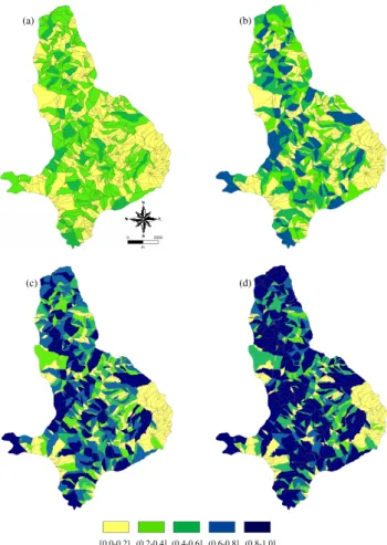
Fig-(b)
(d)
[0.0-0.2] (0.2-0.4] (0.4-0.6] (0.6-0.8] (0.8-1.0]
(c) (a)
Fig. 4. Exceedance probability of landslide temporal occurrence obtained computing the mean recurrence interval of past landslide events from the multi-temporal inventory map (Fig. 2), assuming it will remain the same for the future, and adopting a Poisson proba-bility model. Exceedance probaproba-bility shown for four periods: (a) 5 years, (b) 10 years, (c) 25 years, and (d) 50 years. Square bracket indicates class limit is included; round bracket indicates class limit is not included.
ure 4 shows the exceedance probability of landslide occur-rence for four different periods, from 5 to 50 years. We will use these statistics to ascertain landslide hazard. Table 4 lists the number and total area of slope units in five classes of the estimated probability of temporal landslide occurrence. 5.3 Landslide susceptibility
(g)
[0.0-0.2] (0.2-0.45] (0.45-0.55] (0.55-0.8] (0.8-1.0]
(a) (b) (c)
(d) (e) (f)
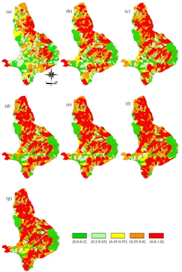
Fig. 5. Landslide susceptibility models obtained through discrimi-nate analysis of the same set of independent thematic variables (Ta-ble 5) and changing the landslide inventory map (dependent vari-able, Fig. 2 and Table 2). (a) Model obtained using landslides iden-tified in the period A1; (b) model obtained using landslides in the period A1–A2; (c) model obtained using landslides in the period A1–B2; (d) model obtained using landslides in the period A1–C2;
(e) model obtained using landslides in the period A1–D2; (f) model
obtained using landslides in the period A1–E2; (g) model obtained using landslides in the period A1–F3. Colours indicate spatial prob-ability in 5 classes. Square bracket indicates class limit is included; round bracket indicates class limit is not included.
area in each slope unit. We selected a threshold of 3% of landslide area to determine if a slope unit was: (i) free of landslides (≤3%) group 0, or (ii) contained slope failures (>3%) group 1. We selected this threshold to account for possible mapping, drafting and digitizing errors in the com-pilation of the landslide inventory map.
Figure 5 shows seven susceptibility maps obtained from seven statistical models prepared using the same set of envi-ronmental variables, and changing incrementally the land-slide inventory map. We prepared the first susceptibility model (Fig. 5a) using only the old landslides (A1 in Ta-ble 2). We then added to the inventory the landslides identi-fied as active in the 1941 aerial photographs and we obtained
a new estimate of the probability of spatial landslide occur-rence (Fig. 5b). We repeated the same procedure adding the slope failures that we identified and mapped using the 1954, 1977, 1985, and 1997 aerial photographs (Figs. 5c–f). To prepare the last model (Fig. 5g), we added all the slope fail-ures mapped in the field in the period from 1998 to 2004.
At each step, we obtained a different susceptibility map, i.e., a different estimate of the probability of landslide spa-tial occurrence,P (S). At each step, a different discriminant function selected different variables as the best predictors of landslide occurrence. Table 5 lists the variables entered in the seven discriminant models. In this table, the standard discriminant function coefficients (SDFC) show the relative importance of each variable in the discriminant function as a predictor of slope stability or instability. Variables with large coefficients, in absolute value, (shown in bold), are strongly associated with the presence/absence of landslides. In particular, positive coefficients are correlated to the ab-sence of landslides, and negative coefficients are correlated to the presence of landslides.
Inspection of Table 5 reveals that two variables (CARBO and TR2) entered all seven discriminant models, and five variables (ORDER, ELV STD, CARBO, FRA, TR2) entered six discriminant models. Further inspection of Table 5 in-dicates that eleven of the 46 thematic variables (23.9%) en-tered at least five susceptibility models, confirming their im-portance in explaining the geographical distribution of past landslides. These variable include morphological (ORDER, SLO AREA, ELV STD, ANG STD, ANGLE3, CC, TR2), lithological (ALLUVIO, CARBO, TRAVERTI), and struc-tural (FRA) conditions. Five variables entered at least five models with large standard discriminant function coefficients (SDFC>|0.300|). Of the latter variables, three are associ-ated with stable conditions (ANG STD, CC, CARBO), and two variables are associated with unstable slope conditions (ELV STD, ANGLE3).
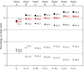
Figure 6 compares the fitting performances of the seven susceptibility models. By upgrading the landslide inventory, the total number of mapping units correctly classified – a measure of model fit – increased from 73.8% to 83.0%. This confirms that a more complete inventory improves the model fit (Guzzetti et al., 2005). Further inspection of Fig. 6 reveals that the two most significant improvements in terms of fitting performance occurred: (i) when the 713 landslides identified as active in the 1941 aerial photographs (A2)were added to the inventory A1, and (ii) when the 413 landslides identified as active in the 1997 (E2)aerial photographs were added to the inventory A1–E1. These new landslides represent an in-crease of 70.59% in number and 18.92% in area (A2), and 16.21% in number and 1.58% in area (E2), with respect to the previous inventories, respectively.
A1 A1-A2 A1-B2 A1-C2 A1-D2 A1-E2 A1-F3 70.3 70.7 69.3
67.6 68.9 67.6
26.9 29.3 30.7
32.4 31.1 32.4
15.3 16.2 14.6 13.5
10.1 10.2 84.7 83.8 85.4 86.5 89.9 89.8
78.4 78.6 79.7 80.1
83.3
73.1
29.7
25.0 75.0 73.8
83.0
0 20 40 60 80 100
Percentage of slope units
Model A
Model B
Model C
Model D
Model E
Model F
Model G
Fig. 6. Degree of fit for seven landslide susceptibility models. x-axis identifies the model, and y-x-axis shows percentage of mapping units in each model. Large red squares: overall percentage of map-ping units correctly classified by the 7 susceptibility models. Black and open symbols show mapping units correctly and incorrectly classified, respectively. Black diamonds show percentage of map-ping units free of landslides classified as stable. Black squares show percentage of mapping units having landslides classified as unsta-ble. Open circles show percentage of mapping units free of land-slides misclassified as unstable (type 1 error). Open triangles show percentage of mapping units having landslides misclassified as sta-ble (type 2 error).
to 2004, the model fitting performance did not improve; it decreased 0.3% (from 83.3% to 83.0%).
Based on the results shown in Fig. 6, we selected model E (Fig. 5e) as the predictor of landslide susceptibility in the Collazzone area, and we adopted this model to determine landslide hazard. We selected model E as a compromise be-tween model performance and the amount of landslide infor-mation used to construct the model. Model E was prepared using 2044 landslides (74.1%) in the period from pre-1941 to 1985 (A1–D2), which allowed using a considerable number of landslides (716, 25.9%) occurred in the period from 1985 to 2004 (E1–F3)for the validation of the prediction skill of the susceptibility model.
For the selected susceptibility model, we attempted an as-sessment of the uncertainty (i.e., the error) associated with the susceptibility estimate. To accomplish this, we prepared an ensemble of 50 susceptibility models obtained from the same set of 46 independent thematic variables and the same multi-temporal landslide map (A1–E2), but using 50 differ-ent and randomly selected subsets of slope units. Each subset contained 760 slope units, i.e., 85% of the entire set of slope units. Next, we prepared a landslide susceptibility model for each subset, obtaining 50 different susceptibility models, i.e., 50 forecasts of landslide susceptibility for the Collaz-zone area.
Slope unit mean probability value
Slope unit single probability value
0.0 0.2 0.4 0.6 0.8 1.0
0.0 0.2 0.4 0.6 0.8 1.0
Fig. 7. Red dots show the relationship between the average value of 50 probability estimates obtained using randomly selected sub-sets of 760 mapping units (85% of total number of map units) (x-axis), and the single probability value obtained for the susceptibility model shown in Fig. 5e (y-axis). Correlation coefficient, r2=0.9876. See text for explanation.
Probability of landslide spatial occurrence
0.0 0.2 0.4 0.6 0.8 1.0
0.16
0.12
0.08
0.04
0
2 standard deviations
low susceptibility
high susceptibility
Fig. 8. Landslide susceptibility model error. The graph shows, for each of the 894 mapping units, the mean value of 50 prob-ability estimates (x-axis) against two standard deviations (2σ )of the probability estimate (y-axis). Along x-axis mapping units are ranked from low (left, green) to high (right, red) spatial probability of landslide occurrence. Colours indicate spatial probability in the same 5 classes shown in Fig. 5. Thick blue line shows estimated model error obtained by linear regression fit. Correlation coeffi-cient, r2=0.8416. See text for explanation.
[0.000-0.015] (0.015-0.030] (0.03-0.045] (0.045-0.060] (0.060-0.080]
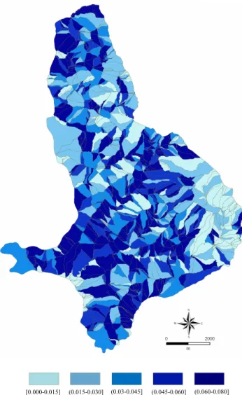
Fig. 9. Map showing estimated model error (2σ )for the
suscepti-bility model shown in Fig. 5e. Model error computed using Eq. (3) is shown in 5 classes. Square bracket indicates class limit is in-cluded; round bracket indicates class limit is not included. See text for explanation.
with the single probability estimate obtained for the model shown in Fig. 5e (y-axis), which was prepared using the en-tire set of 894 slope units. The correlation between the two estimates of landslide susceptibility is very high (r2=0.9876). This is indication that the two classifications – despite some scatter – are very similar. Based on this result, we prepared Fig. 8 that shows, for the 894 slope units, the relationship between the ranking of landslide susceptibly (x-axis) and 2 standard deviations (2σ )of the probability estimate (y-axis). Inspection of Fig. 8 reveals that the measure of 2σ is low (<0.05) for slope units classified as highly susceptible (prob-ability>0.80) and as largely stable (probability<0.20). The scatter in the probability estimate is larger for intermediate values of the probability (i.e., between 0.40 and 0.60). This indicates that for slope units having intermediate values of probability, not only is model E incapable of satisfactorily classifying the terrain as stable or unstable, but also that the
[0.00-0.02] (0.02-0.04] (0.04-0.06] (0.06-0.08] (0.08-0.10] (0.10-0.30] (0.30-0.50] (0.50-0.70] (0.70-1.00]
10 years 5 years
25 years
50 years
AL≥1×10³m2 AL≥1×10⁴m2
Fig. 10. Examples of landslide hazard maps for four periods, from 5 to 50 years (from top to bottom), and for two landslide sizes,AL≥ 1000 m2(left) andAL≥10 000 m2, i.e. 1 ha (right). Colours show different joint probabilities of landslide size, of landslide temporal occurrence, and of landslide spatial occurrence (susceptibility).
obtained estimate is highly variable and, most probably, un-reliable. The variation in the probability estimate of landslide susceptibility can be approximated by the following equa-tion, obtained by linear regression fit (least square method): y= −0.3218x2+0.3212x 0≤x ≤1 (r2=0.8416)(3) where,x is the estimated value of the probability of pertain-ing to an unstable slope unit, andyis the corresponding 2σ of the probability estimate.
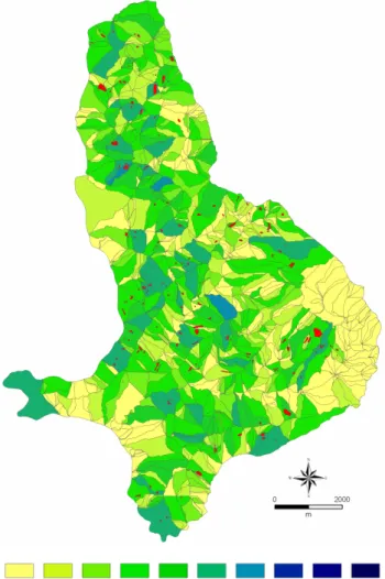
[0.0-0.1] (0.1-0.2] (0.2-0.3](0.3-0.4](0.4-0.5](0.5-0.6] (0.6-0.7](0.7-0.8] (0.8-0.9] (0.9-1.0]
Fig. 11. Exceedance probability of landslide temporal occurrence in the 7-year period from 1998 to 2004 (F1–F3)based on the record of landslide occurrence in the period between 1941 and 1997 (A2– E2) obtained from the multi-temporal inventory. Square bracket indicates class limit is included; round bracket indicates class limit is not included.
landslide susceptibility assessment provided by model E, and shown in Fig. 5e.
5.4 Landslide hazard
We now have all the information required to determine quan-titatively landslide hazard in the study area. We use:
(i) the probability of landslide size, a proxy for landslide magnitude, obtained from the statistical analysis of the frequency-area distribution of the mapped landslides (Fig. 3),
(ii) the probability of landslide occurrence for established periods, obtained by computing the mean recurrence in-terval between successive failures in each mapping unit, and adopting a Poisson probability model (Fig. 4, Ta-ble 4), and
Cumulative landslides (%)
Exceedence probability
010 20 30 40 50 60 70 80 90 100
0.0 0.1 0.2 0.3 0.4 0.5 0.6 0.7
Fig. 12. Estimate of the prediction skill of the temporal forecast shown in Fig. 11. x-axis shows classes of the temporal probability obtained considering landslides in the period from 1941 to 1997 (A2–E2). y-axis shows cumulative percentage of landslide area and landslide number in the period from 1998 to 2004 (F1–F3). Red line shows cumulative percentage of landslide area. Blue line shows cumulative percentage of landslide number.
(iii) the spatial probability of slope failures (i.e., susceptibil-ity) obtained through discriminant analysis of 46 envi-ronmental variables (Fig. 5).
Assuming independence, we multiply the three probabilities and we obtain landslide hazard, i.e., the joint probability that a mapping unit will be affected by future landslides that ex-ceed a given size, in a given time, and because of the lo-cal environmental setting. Figure 10 shows examples of the obtained landslide hazard assessment. This figure portrays landslide hazard for four periods (i.e., 5, 10, 25 and 50 years), and for two different landslide sizes, greater or equal than 1×10³m2, and greater or equal than 1×10³m4(1 ha).
6 Model validation
0 20 40 60 80 0 20 40 60 80
Area in susceptibility class (%)
Landslide area in
susceptibility class (%)
(a)
0 20 40 60 80 100
Landslide area in
susceptibility class (%)
Area in susceptibility class (%) 0
20 40 60 80 100
(b)
0 20 40 60 80
0 20 40 60 80 100
(c)
Landslide area in
susceptibility class (%)
Area in susceptibility class (%)
0 20 40 60 80
0 20 40 60 80 100
Landslide area in
susceptibility class (%)
(d)
Area in susceptibility class (%)
0 20 40 60 80
0 20 40 60 80 100
Landslide area in
susceptibility class (%)
(e)
Area in susceptibility class (%)
0 20 40 60 80
0 20 40 60 80 100
Landslide area in
susceptibility class (%)
(f)
Area in susceptibility class (%)
0 20 40 60 80
0 20 40 60 80 100
Landslide area in
susceptibility class (%)
(g)
Area in susceptibility class (%)
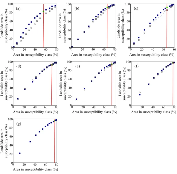
Fig. 13. Comparison of the susceptibility model fit and prediction performance. In the graphs, x-axes show the percentage of study area in each susceptibility class, ranked from most (left) to least (right) susceptible, and y-axes show the percentage of landslide area in each susceptibility class. Filled symbols measure the degree of model fit and open symbols measure the prediction skill of the susceptibility models. Red lines show 0.5 probability threshold, separating unstable (P (S)<0.5) and stable (P (S)>0.5) slope units.
occurrence in the 7-year period from 1998 to 2004 (Fig. 11). We then counted the number of landslides occurred in the pe-riod in each probability class. Results are shown in Fig. 12. In the 7-year considered period, the largest expected proba-bility of landslide occurrence is 0.7, indicating that nowhere in the study area landslides are expected to be “certain” in the period. Most of the mapped landslides (∼79%) and most of the landslide areas (∼81%) occurred in slope units with an expected probability of experiencing landslides ranging between 0.3 and 0.6. This is not a bad result, considering the difficulty of the task, and in particular considering: (i) the comparatively limited number of landslides occurred in the short validation period, (ii) the simplicity of the adopted Poisson model, and (iii) the temporal variability of landslide phenomena in the examined period.
Next, we attempted a validation of the spatial forecast of landslide occurrence, i.e., of landslide susceptibility. To ac-complish this, we computed the total area of new landslides
threshold, i.e., the limit between slope units classified as un-stable (P (S)<0.5) or un-stable (P (S)>0.5) by the discriminant functions.
Inspection of Fig. 13 reveals that for models A, B and C, prepared using landslides A1, A1–A2 and A1–B2, respec-tively, model fit (filled symbols) is significantly better than model prediction skill (open symbols). The difference be-tween degree of model fit and model prediction skill de-creases for the other models. We attribute the reduced differ-ence to the increased number of landslides used to prepare the models, which corresponds to a larger proportion of the study area affected by slope failures. The percentage of terri-tory classified as unstable by the seven susceptibility models increases from 55.6% (model A, A1)to 76.6% (model F, A1– E2). Table 6 shows similar results. In this table, each block row corresponds to a susceptibility model and lists the per-centage and the total landslide area mapped in a given period that falls in five classes of landslide susceptibility, from very high (VH) to very low (VL) susceptibility. The figures indi-cate how well a model was capable of predicting future land-slides. All the models correctly classified as landslide prone more than 50% of the areas where “future” (with respect to the model) landslides occurred. As an example, model A (first block row in Table 6), which was prepared using only 270 landslides older than 1941 (A1), was capable of predict-ing 63.6% of all the landslides recognized as active in 1941 (A2)and which occurred within high (H, 41.4%) and very high (VH, 22.2%) susceptibility classes. Model A misclas-sified 23.5% of the landslide areas occurred in 1941 in slope units classified of low (L, 20.6%) or very low (VL, 2.9%) susceptibility. Model A performed less efficiently in pre-dicting landslides occurred in the period from 1955 to 1977 (C1–C2). For this period, the model was capable of correctly predicting 57.7% of the new landslides, and failed to predict 31.3% of the slope failures that occurred in low (24.4%) and in very low (6.9%) susceptibility areas. It is useful to check the ability of Model A to predict the location of the most recent landslides occurred in the Collazzone area, i.e., the landslides mapped in the period from 1998 to 2004 (F1–F3). For this period, model A was capable of correctly predicting 58.1% of the new landslides, and failed to predict 30.6% of the slope failures that occurred in low (25.0%) and in very low (5.6%) susceptibility areas. Considering that model A was prepared using only 270 landslides, and considering the time elapsed from model “prediction” (1941) to model “ver-ification” (2004), performance of the model should be con-sidered satisfactory.
Data listed in Table 6 can also be used to determine the contribution of new landslides to the model prediction skills. Considering the last column, one can see that model A was capable of predicting 58.1% of the landslides occurred in the period from 1998 to 2004 (F1–F3), whereas model E cor-rectly predicted 89.7% of the landslides in the same period, with the majority of the slope failures (61.4%) falling in the very high susceptibility class and only 2.0% of the landslides occurring in the very low susceptibility class.
7 Discussion
The adopted landslide hazard model holds under a set of as-sumptions (Guzzetti et al., 2005), namely that: (i) landslides will occur in the future under the same circumstances and because of the same factors that produced them in the past, (ii) landslide events are independent (uncorrelated) random events in time, (iii) the mean recurrence of slope failures will remain the same in the future as it was observed in the past, (iv) the statistics of landslide area do not change in time, (v) landslide area is a reasonable proxy for landslide magnitude, and (vi) the probability of landslide size, the probability of landslide occurrence for established periods, and the spatial probability of slope failures, are all independent. We now discuss the validity of these assumptions for the Collazzone study area. We anticipate that the results are not significantly different from the results obtained previously in the northern Italian Apennines (Guzzetti et al., 2005).
That landslides will occur in the future under the same conditions and because of the same factors that triggered them in the past – a consequence of the principle of uni-formitarianism – is a recognized postulate for all functional susceptibility or hazard assessments (Carrara et al., 1991; Hutchinson, 1995; Aleotti and Chowdhury, 1999; Chung and Fabbri, 1999; Guzzetti et al., 1999). This assumption has ge-omorphological limitations (Guzzetti et al., 2005). First-time failures occur under conditions of peak resistance (friction and cohesion), whereas landslide reactivations occur under intermediate or residual conditions. Slope failures change the morphology of the terrain where the failures occur, and when a landslide moves, it may change the hydrological con-ditions of the slope. Further, landslides can change their type of movement and velocity with time. Lastly, landslide occur-rence and abundance are a function of environmental condi-tions that vary with time at different rates. Some of these environmental variables are affected by human actions (e.g., land use, deforestation, irrigation, etc.), which are also highly changeable. Because of these complications, each landslide occurs in a distinct local environmental context. Despite the inherent limitations, in this work we have assumed that in the study area future landslides will occur on average under the same circumstances and because of the same conditions that triggered them in the past. We further assumed that our knowledge of the distribution of past failures was reasonably accurate and complete.
Table 6. Validation of landslide susceptibility models prepared for the Collazzone area. Susceptibility classes are: VH, very high [1.0–0.8); H, high [0.8–0.6); U, uncertain [0.6–0.4); L, low [0.4–0.2); and VL, very low [0.0–0.2]. Square bracket indicates class limit is included; round bracket indicates class limit is not included. See text for explanation.
Landslides
Susceptibility A2 B1–B2 C1–C2 D1–D2 E1–E2 F1–F3
class m2 % m2 % m2 % m2 % m2 % m2 %
Model A VH 911 140.6 22.2 270 108.7 23.9 454 661.6 21.1 198 483.3 18.7 180 541.5 17.4 158 462.5 23.1 (A1) H 1 697 192.4 41.4 403 642.4 35.8 787 829.8 36.6 459 594.8 43.4 458 563.8 44.2 240 365.7 35.0 U 528 725.9 12.9 127 781.7 11.3 234 966.3 10.9 116 624.4 11.0 97 879.6 9.4 78 145.6 11.4 L 843 823.1 20.6 261 978.1 23.2 525 874.0 24.4 241 526.1 22.8 213 053.2 20.5 171 694.4 25.0 VL 117 690.9 2.9 65 517.8 5.8 147 766.3 6.9 42 881.7 4.0 87 558.2 8.4 38 142.0 5.6
Model B VH 541 984.9 48.0 992 951.9 46.2 542 926.3 51.3 480 519.6 46.3 308 755.7 45.0 (A1–A2) H 371 180.2 32.9 685 888.0 31.9 363 631.1 34.3 379 343.5 36.6 189 673.3 27.6
U 101 845.1 9.0 159 079.9 7.4 44 413.2 4.2 67 523.6 6.5 80 850.9 11.8 L 86 376.4 7.7 263 763.8 12.3 88 732.4 8.4 61 269.9 5.9 84 186.9 12.3 VL 27 642.0 2.4 49 414.4 2.3 19 407.4 1.8 48 939.8 4.7 23 343.3 3.4
Model C VH 1 016 348.7 47.2 535 420.5 50.6 562 019.0 54.2 309 502.5 45.1 (A1–B2) H 707 578.8 32.9 325 653.6 30.7 318 229.8 30.7 230 271.7 33.5
U 106 075.3 4.9 99 624.3 9.4 40 110.7 3.9 40 036.0 5.8
L 275 302.8 12.8 90 518.6 8.5 73 078.6 7.0 86 976.5 12.7
VL 45 792.3 2.1 7893.5 0.7 44 158.2 4.3 20 023.4 2.9
Model D VH 716 215.8 67.6 733 293.9 70.7 413 097.3 60.1
(A1–C2) H 252 034.5 23.8 191 491.7 18.5 199 123.4 29.0
U 21 060.9 2.0 17 116.3 1.6 20 407.3 3.0
L 49 859.5 4.7 52 290.9 5.0 34 293.2 5.0
VL 19 939.8 1.9 43 403.6 4.2 19 888.8 2.9
Model E VH 697 304.1 67.2 421 936.4 61.4
(A1–D2) H 232 577.8 22.4 194 225.1 28.3
U 19 079.0 1.8 31 693.8 4.6
L 50 110.9 4.8 25 008.2 3.6
VL 38 524.5 3.7 13 946.5 2.0
Model F VH 478 955.5 69.7
(A1–E2) H 159 285.7 23.2
U 24 279.4 3.5
L 10 343.0 1.5
VL 13 946.5 2.0
changes are not expected. Inspection of Table 5 indicates that 29 of the 32 thematic variables entered into the suscepti-bility models are not expected to change significantly in the considered period. However, land use types (three variables, BOSCO, SA, FRUTT) may change significantly in the pe-riod. In a representative portion of the Collazzone area, com-parison of land-use maps obtained form aerial photographs taken in 1941 (B in Table 1) and aerial photographs taken in 1999, revealed a reduction of about 65% of the forest cov-erage in the 57-year period, in favour chiefly of cultivated land. In the same period, agricultural practices have changed significantly, largely aided by new mechanical equipments. In the central Apennines, areas recently deforested for agri-cultural purposes are generally more prone to shallow land-slides. If this will be the case for the Collazzone area, some of the environmental variables considered in the susceptibil-ity model will change, possibly hampering the validsusceptibil-ity of the model, and new variables describing land use change should be considered to forecast the location of new slope failures.
The available susceptibility model (Fig. 5e, Table 5) does not consider the landslide triggering factors, i.e., rainfall, seismic shaking or snow melting. Changes in the frequency or inten-sity of the driving forces will not affect (at least not in the considered period) the susceptibility model. However, they may affect the rate of occurrence of landslide events.
Analysis of the historical record of damaging landslide events in Umbria indicates that in the 85-year period from 1917 to 2001, 1497 landslide events occurred at 1286 differ-ent sites, with only 75 sites affected two or more times, and only one site affected four times. Based on this historical record, the same landslide site was affected on average 1.16 times, indicating a low rate of recurrence of landslide events at the same site. Despite known incompleteness of the histor-ical record (Guzzetti et al., 2003; Guzzetti and Tonelli, 2004), the obtained findings concur to determine that for the period of our hazard assessment (50 years), in the Collazzone area landslides can be considered uncorrelated random events in time.
Further analysis of the historical record of landslide events in Umbria reveals that of the 889 events for which the trig-gering mechanism is known, the majority (720, 80.9%) were the result of intense rainfall. The remaining landslide events were due to rapid snow melting (37, 4.2%), infiltration (135, 15.2%), earthquake shaking (38, 4.3%), erosion of the toe of the slope (59, 6.6%), human actions on artificial slopes (81, 9.1%), and other causes (39, 4.3%). The statistics indi-cates that meteorological triggers (rainfall and snow melting) cause most of the landslides in Umbria (and in the Collaz-zone area). If the rate of occurrence of the meteorological events that trigger landslides changes, the mean rate of slope failures will also change. If the intensity (amplitude and du-ration) of the rainfall will change, the rate of slope failures might change, in a way that is not easily predictable. Modi-fications in land use induced by changes in agricultural prac-tices may also change the rate of occurrence of landslides.
Determining the statistics of landslide areas is no trivial task (Malamud et al., 2004). The (scant) available informa-tion indicates that the frequency-area statistics of landslide areas does not change significantly across lithological or physiographical boundaries. Malamud et al. (2004) showed that three different populations of landslides produced by dif-ferent triggers (i.e., seismic shaking, intense rainfall, rapid snow melting) in different physiographical regions (southern California, central America, central Italy), exhibit virtually identical probability density functions. Unpublished work conducted in central Italy indicates that for the same phys-iographical region the probability density of landslide area does not change significantly in time. It is therefore safe to assume that in the Collazzone area the frequency-area statis-tics of landslide area will not change in the 50-year period of the hazard assessment. Since the most abundant landslides in the study area are small (∼1×10³m2, Fig. 3a), great care must be taken in mapping accurately the small slope failures. The slope of the heavy tail of the probability density distri-bution shown in Fig. 3a is controlled by a limited number of landslides. There are 23 landslides (0.82%) larger than 1×10⁵m2 and only one landslide (0.03%) larger than one square kilometre. Care must be taken in mapping the largest landslides, and in deciding whether they represent an indi-vidual slope failure or the result of two or more coalescent landslides.
No unique measure of landslide magnitude is available. Hungr (1997) proposed to use destructiveness as a measure of landslide magnitude. In this work, we have adopted land-slide area as a proxy for landland-slide destructiveness and of landslide magnitude. We obtained the area of the individ-ual slope failures from the multi-temporal landslide inven-tory. To determine if landslide area is a reasonable measure of landslide destructiveness in the Collazzone area we have analysed the historical catalogue of damaging slope failures in Umbria. Information on the size (area, length, width) of landslides is available for 344 events (22.9%), which range from 1.0×10³m2 to more than one square kilometre (mean=1.64×10⁴m2). Damage caused by these landslides was mostly to the road network (73 events) and, subordi-nately, to private homes (53 events) and to the infrastructure (30 events). Twenty-two landslide events produced casual-ties, and 12 landslides produced 22 fatalicasual-ties, none of which in the Collazzone area. Information on the landslide type is available for 368 events (24.6%), of which 152 were slides, 31 flows and 148 falls. Slides and flows caused the most se-vere damage, and falls produced minor interruptions along the roads. As a whole, the available historical information on damaging slope failures in Umbria concurs to establish that: (i) damage in the Collazzone area is expected mostly from slow to rapid moving slides and flows, i.e., the type of failures considered in the hazard assessment, and (ii) large landslides are expected to produce a larger damage, particu-larly to roads and private buildings in old villages and single dwellings.
The last assumption of the adopted hazard model is that the probabilities of landslide sizeP (AL), of temporal occur-renceP (NL), and of spatial incidence of mass movements P (S) are independent. The legitimacy of this assumption is difficult to prove. We have shown that the probability of landslide area is largely independent from the physiograph-ical setting. As a first-approximation, it is safe to conclude that the probability of landslide area is independent from sus-ceptibility. The susceptibility model was constructed without considering the driving forces (meteorological or else) that control the rate of occurrence of slope failures in the study area. We conclude that the rate of landslide events is in-dependent from susceptibility. The catalogue of historical damaging landslides reveals that landslides occurred in all sizes. We consider this an indication that the rate of failures is independent from landslide size.
8 Concluding remarks
hazard from a detailed multi-temporal inventory map, pre-pared through the interpretation of five sets of aerial pho-tographs and field surveys. The adopted model proved ap-plicable in the test area. We judge the model appropriate in similar areas, and chiefly where a multi-temporal landslide inventory captures the types, sizes, and expected recurrence of slope failures. We tested the model ability to predict the location of new or reactivated landslides, and the predicted temporal occurrence of the slope failures. We found the for-mer better than the latter, confirming the difficulty in predict-ing when or how frequently slope failures will occur in an area.
We conclude by pointing out that the main scope of a landslide hazard assessment is to provide probabilistic ex-pertise on future slope failures to planners, decision makers, civil defence authorities, insurance companies, land devel-opers, and individual landowners. The adopted method al-lowed us to prepare a large number of different hazard maps (Fig. 10), depending on the adopted susceptibility model, the established period, and the minimum size of the expected landslide. How to combine such a large number of hazard scenarios efficiently, producing cartographic, digital, or the-matic products useful for the large range of interested users, remains an open problem that needs further investigation. Acknowledgements. Work supported by CNR IRPI and Riskaware
(Interreg III-C CADSES Programme) grants. CNR GNDCI publication number 2905.
Edited by: L. Ferraris
Reviewed by: N. Casagli and another referee
References
Aleotti, P. and Chowdhury, R.: Landslide hazard assessment: sum-mary review and new perspectives, Bull. Engi. Geology and the Environ., 58, 21–44, 1999.
Barchi, M., Brozzetti, F., and Lavecchia, G.: Analisi strutturale e geometrica dei bacini della media valle del Tevere e della valle umbra, (in Italian), Bollettino Societ`a Geologica Italiana, 110, 65–76, 1991.
Canuti, P. and Casagli, N.: Considerazioni sulla valutazione del ris-chio di frana. CNR – GNDCI Pubblication number 846, Proceed-ings conference Fenomeni franosi e centri abitati, Bologna, 27 May 1994, CNR – GNDCI and Regione Emilia-Romagna, (in Italian), 29–130, 1994.
Cardinali, M., Ardizzone, F., Galli, M., Guzzetti, F., and Re-ichenbach, P.: Landslides triggered by rapid snow melting: the December 1996–January 1997 event in Central Italy, Proceed-ings 1st Plinius Conference on Mediterranean Storms, edited by: Claps, P. and Siccardi, F., Bios Publisher, Cosenza, 439–448, 2002a.
Cardinali, M., Reichenbach, P., Guzzetti, F., Ardizzone, F., An-tonini, G., Galli, M., Cacciano, M., Castellani, M., and Salvati, P.: A geomorphological approach to estimate landslide hazard and risk in urban and rural areas in Umbria, central Italy, Nat. Hazards Earth Syst. Sci., 2, 57–72, 2002b,
SRef-ID: 1684-9981/nhess/2002-2-57.
Carrara, A.: A multivariate model for landslide hazard evaluation, Mathematical Geology, 15, 403–426, 1983.
Carrara, A., Cardinali, M., Detti, R., Guzzetti, F., Pasqui, V., and Reichenbach, P.: GIS Techniques and statistical models in eval-uating landslide hazard, Earth Surface Processes and Landform, 16, 5, 427–445, 1991.
Carrara, A., Cardinali, M., Guzzetti, F., and Reichenbach, P.: GIS technology in mapping landslide hazard, in: Geographical Infor-mation Systems in Assessing Natural Hazards, edited by: Car-rara, A. and Guzzetti, F., Kluwer Academic Publisher, Dordrecht, The Netherlands, 135–175, 1995.
Chung, C. J. and Frabbri, A. G.: Probabilistic prediction models for landslide hazard mapping, Photogrammetric Engineering & Remote Sensing, 65, 12, 1389–1399, 1999.
Cencetti, C.: Il Villafranchiano della “riva umbra” del F. Tevere: elementi di geomorfologia e di neotettonica. Bollettino Societ`a Geologica Italiana, (in Italian), 109, 2, 337–350, 1990.
Coe, J. A., Michael, J. A., Crovelli, R. A., and Savage, W. Z.: Pre-liminary map showing landslide densities, mean recurrence in-tervals, and exceedance probabilities as determined from historic records, Seattle, Washington, United States Geological Survey Open File Report 00-303, 2000.
Conti, M. A. and Girotti, O.: Il Villafranchiano nel “Lago Tiberino”, ramo sud-occidentale: schema stratigrafico e tettonico, Geolog-ica Romana, (in Italian), 16, 67–80, 1977.
Crovelli, R. A.: Probability models for estimation of number and costs of landslides, United States Geological Survey Open File Report 00-249, 2000.
Cruden, D. M. and Varnes, D. J.: Landslide types and processes, in: Landslides, Investigation and Mitigation, edited by: Turner, A. K. and Schuster, R. L., Transportation Research Board Special Report 247, Washington D.C., 36–75, 1996.
Einstein, H. H.: Special lecture: Landslide risk assessment pro-cedure, in: Landslides, edited by: Bonnard, C., 2, 1075–1090, 1988.
Guzzetti, F. and Cardinali, M.: Carta Inventario dei Fenomeni Fra-nosi della Regione dell’Umbria ed aree limitrofe, CNR Gruppo Nazionale per la Difesa dalle Catastrofi Idrogeologiche Publica-tion n. 204, 2 sheets, scale 1:100 000, (in Italian), 1989. Guzzetti, F. and Cardinali, M.: Landslide inventory map of the
Um-bria region, Central Italy, in: Proceedings ALPS 90 6th Interna-tional Conference and Field Workshop on Landslides, edited by: Cancelli, A., Milan, 12 September 1990, 273–284, 1990. Guzzetti, F., Carrara, A., Cardinali, M., and Reichenbach, P.:
Land-slide hazard evaluation: a review of current techniques and their application in a multi-scale study, Central Italy, Geomorphology, 31, 181–216, 1999.
Guzzetti, F., Malamud, B. D., Turcotte, D. L., and Reichenbach, P.: Power-law correlations of landslide areas in Central Italy, Earth and Planetary Science Letters, 195, 169–183, 2002.
Guzzetti, F., Reichenbach, P., Cardinali, M., Ardizzone, F., and Galli, M.: Impact of landslides in the Umbria Region, Central Italy, Nat. Hazards Earth Syst. Sci., 3, 469–486, 2003,
SRef-ID: 1684-9981/nhess/2003-3-469.
Guzzetti, F., Reichenbach, P., Ardizzone F., Cardinali, M., and Galli, M.: Probabilistic landslide hazard assessment at the basin scale, Geomorphology, 72, 272–299, 2005.
Guzzetti, F. and Tonelli, G.: SICI: an information system on histor-ical landslides and floods in Italy, Nat. Hazards Earth Syst. Sci., 4, 213–232, 2004,
Hungr, O.: Some methods of landslide hazard intensity mapping, in: Landslide risk assessment, edited by: Cruden, D. M. and Fell, R., Balkema Publisher, Rotterdam, 215–226, 1997.
Hutchinson, J. N.: Keynote paper: Landslide hazard assessment, in: Landslides, Balkema, Rotterdam, edited by: Bell, D. H., 1805– 1841, 1995.
Keaton, J. R., Anderson, L. R., and Mathewson, C. C.: Assessing debris flow hazards on alluvial fans in Davis County, Utah, in: Proceedings 24th Annual Symposium on Engineering Geology and Soil Engineering, edited by: Fragaszy, R. J., Pullman, Wash-ington State University, 89–108, 1988.
Lips, E. W. and Wieczorek, G. F.: Recurrence of debris flows on an alluvial fan in central Utah, in: Hydraulic/Hydrology of Arid Lands, edited by: French, R. H., Proceedings of the Interna-tional Symposium, American Society of Civil Engineers, 555– 560, 1990.
Malamud, B. D., Turcotte, D. L., Guzzetti, F., and Reichenbach, P.: Landslide inventories and their statistical properties, Earth Surface Processes and Landforms, 29, 6, 687–711, 2004. McCalpin, J.: Preliminary age classification of landslides for
inven-tory mapping: 21st Annual Symposium on Engineering Geology and Soils Engineering, 5–6 April 1984, Pocatello, Idaho, 13 p., 1984.
Reichenbach, P., Galli, M., Cardinali, M., Guzzetti, F., and Ardiz-zone, F.: Geomorphologic mapping to assess landslide risk: con-cepts, methods and applications in the Umbria Region of central Italy, in: Landslide risk assessment, edited by: Glade, T., Ander-son, M., and Crozier, M. J., John Wiley, 429–468, 2005.
Servizio Geologico Nazionale: Carta Geologica dell’Umbria. Map at 1:250 000 scale, (in Italian), 1980.
Soeters, R. and van Westen, C. J.: Slope instability recognition analysis and zonation, in: Landslide investigation and mitiga-tion, edited by: Turner, A. K. and Schuster, R. L., National Re-search Council, Transportation ReRe-search Board Special Report 247, Washington, 129–177, 1996.
Stark, C. P. and Hovius, N.: The characterization of landslide size distributions, Geophys. Res. Lett., 28, 6, 1091–1094, 2001. van Westen, C. J.: GIS in landslide hazard zonation: A review with
examples from the Colombian Andes, in: Taylor and Francis, edited by: Price, M. F. and Heywood, D. I., London, 135–165, 1994.
Varnes, D. J. and IAEG Commission on Landslides and other Mass-Movements: Landslide hazard zonation: a review of principles and practice, UNESCO Press, Paris, 63 p., 1984.