Introduction
A mixed-use development is a single physically and functionally integrated development of three or more revenue-producing uses developed in conformance with a coherent plan. Because the diversity of land uses is believed to provide a multifunctional living space and allows for a more efficient utilization of urban land and a reduced distance between origin and destination, mixed-use has become a widely accepted trip reduction strategy included in many transportation plans.
However, thus far, a rigorous and quantitative analysis on the relationship between land-use mixture and trip reduction is still lacking and inconclusive. The assumption that land-use mixture will necessarily lead to reduced trip making is often called into question. In fact, it is usually hard to prove the existence of a positive and causal relationship between mixed land-use and trip reduction due to the confounded effects from other factors.
This study is intended to assess the impacts of mixed-use development on home-based trip rates (person trips per household) in Richmond, Virginia, United States (U.S.). Through this empirical study, the paper will quantify the correlation relationship between land-use mixture, socioeconomic variables, and trip making by means of both geographical and statistical tools. On the geographical front, the paper utilizes the tool of Geographical Information System (GIS), Abstract: Richmond, Virginia has implemented numerous mixed land-use policies to encourage non-private-vehicle commuting for decades based on the best practices of other cities and the assumption that land-use mixture would positively lead to trip reduction. This paper uses both Geographical Information Systems (GIS) and statistical tools to empirically test this hypothesis. With local land use and trip making data as inputs, it first calculates two common indices of land-use mixture - entropy and dissimilarity indices, using GIS tool, supplemented by Microsoft Excel. Afterwards, it uses Statistical Package for Social Sciences (SPSS) to calculate the correlation matrices among land-use mixture indices, socioeconomic variables, and home-based work/other trip rates, followed by a series of regression model runs on these variables. Through this study, it has been found that land-use mixture has some but weak effects on home-based work trip rate, and virtually no effects on home-based other trip rate. In contrast, socioeconomic variables, especially auto ownership, have larger effects on home-based trip making.
Key Words:land-use mixture, socioeconomic variables, home-based trip rates, entropy index, dissimilarity index.
GEOGRAPHICAL AND STATISTICAL ANALYSIS ON THE
RELATIONSHIP BETWEEN LAND-USE MIXTURE AND HOME
–
BASED TRIP MAKING AND MORE: CASE OF RICHMOND,
VIRGINIA
Yin-Shan
MA
1),
Xueming
CHEN
2)supplemented by Microsoft Excel, to calculate entropy and dissimilarity indices for measuring land-use mixture. On the statistical front, the paper relies on Statistical Package for Social Sciences (SPSS) to measure the correlation and regression relationships among home-based trip rates, land-use mixture indices, and socioeconomic variables. Because of its theoretical and practical contributions, this study has its research significance.
Following this introduction, this paper contains five additional sections. Section 2 is a literature review. After that, Section 3 introduces the research methodology. Section 4 then briefly describes the geographical setting of Richmond, Virginia, focusing on its location, demography, land use, poverty, and transportation. As the core component of this paper, Section 5 presents the analytical results calculated using GIS, MS Excel, and SPSS tools. Finally, Section 6 summarizes research findings and draws conclusions.
Literature Review
There is a voluminous literature on the relationship between built environment (BE, which includes the so-called “D” variables, such as density, diversity, design, distance to transit, and others) and travel behavior (TB). Due to the space limitation, this section only provides a concentrated review of the BE-TB relationship, with a particular emphasis on the relationship between mixed use and trip frequencies.
An Overview
Even though the conventional four-step transportation model initially developed in the 1950s already includes the BE factors in the modelling process, the modern systematic studies on the relationship between BE and TB can be traced to the 1980s. In the 1980s, planners realized that the spatial distribution of trip origins and destinations could be used as a policy tool to affect travel. In the space of a few years, this idea was articulated in the form of jobs-housing balance (Cervero 1986,1989), transit-oriented development (Calthorpe 1993), the
transportation elements of the new urbanism and neotraditional design (Duany and Plater–Zyberck 1991, Friedman, Gordon and Peers 1994, Kelbaugh 1989), and the explosive
land use-travel studies from the mid-1990s (see, e.g., Cervero and Kockelman 1997, Ewing, Haliyur and Page 1995, Frank and Pivo 1995). So far, hundreds of papers and several literature reviews have been published (for reviews, see, e.g., Badoe and Miller 2000, Boarnet and Crane 2001, Boarnet 2011, Brownstone 2008, Crane 2000, Ewing and Cervero 2001, 2010, Handy 2005, Heath et al. 2006, Henderson and Bialeschki 2005). The research is still going on because many issues have not been resolved yet.
Research on Mixed Use: Still Inconclusive
complicated nature.
Effects of Mixed Use on Travel: A General Understanding
According to Smart Growth Online, by putting residential, commercial and recreational uses in close proximity to one another, alternatives to driving, such as walking or biking, become viable. Mixed land uses also provide a more diverse and sizable population and commercial base for supporting viable public transit (Source: http://www.smartgrowth.org/principles/ mix_land.php).
National Cooperative Highway Research Program (NCHRP) Program Report 684 holds that mixed-use developments can achieve internal trip capture rates ranging between 0% and 53%, which would reduce traffic volumes on the external roadway system, according to the surveys conducted by Institute of Transportation Engineers (ITE) in 1998 (Transportation Research Board 2011).
Per Litman and Steele (2012), neighborhoods that mix land uses, make walking safe and convenient, and are near other development, allow residents and workers to drive significantly less if they choose. Mixed use is believed to reduce commute distances, particularly if affordable housing is located in job-rich areas, and mixed-use area residents are more likely to commute by alternative modes (Modarres 1993, Kuzmyak and Pratt 2003, Ewing and Cervero 2010, Spears, Boarnet and Handy 2010).
Frank and Pivo (1994) studied the impacts of land-use mix and density on use of the single occupancy vehicles, transit and walk modes, respectively, for shopping and work trips using data from the Puget Sound Transportation Panel, the U.S. Census Bureau and three local agencies in Washington State. From a simple correlation analysis, urban form and mode split were found to be significantly related.
With regard to the magnitude of impacts, based on a detailed review of research, Spears, Boarnet and Handy (2010) concluded that the elasticity of vehicle miles traveled (VMT) with respect to land use mix is -0.02 to -0.11 (a 10% increase in an entropy or dissimilarity index reduces average VMT by 0.2% to 1.1%). Ewing and Cervero (2010) found that land use mix reduces vehicle travel and significantly increases walking. Krizek (2003) found that households located in highly accessible neighborhoods travel a median distance of 3.2 km (2.0 mile) one-way for errands versus 8.1 km (5.0 mile) for households in less accessible locations.
Using travel diary data from the New York/New Jersey/Connecticut regional travel survey, Salon (2006) concluded that the built environment accounted for one half to two thirds of the difference in walking levels associated with changes in population density in most areas of New York City. Using travel diary data from the Austin travel survey, Zhou and Kockelman (2008) found that the built environment accounted for 58% to 90% of the total influence of residential location on VMT, depending on model specifications. Using travel diary data from northern California, Cao (2010) reported that, on average, neighborhood type accounted for 61% of the observed effect of the built environment on utilitarian walking frequency and 86% of the total effect on recreational walking frequency.
More Complicated Issues: Association versus Causality
establish whether the cause precedes the effect. Most studies have controlled for socio-demographic characteristics, thereby minimizing the possibility that other confounding variables such as income or residential self-selection, for example, create a spurious relationship between the built environment and travel behavior.
Over the past few years, Cao, Mokhtarian, Handy and others conducted a series of studies on the residential self-selection issues. They found at least 38 studies using nine different research approaches have attempted to control for residential self-selection (Cao, Mokhtarian,
and Handy 2009, Mokhtarian and Cao 2008). Nearly all of them found “resounding” evidence of
statistically significant associations between the built environment and travel behavior, independent of self-selection influences. However, nearly all of them also found that residential self-selection attenuates the effects of the built environment on travel.
Using data from a regional travel diary survey in Raleigh, North Carolina, Cao, Xu and Fan (2009) estimated that anywhere from 48% to 98% of the difference in VMT was due to direct environmental influences, the balance being due to self-selection.
Using the survey data in eight neighborhoods in Northern California, Handy, Cao and Mokhtarian (2005) shows that a multivariate analysis of cross-sectional data shows that differences in travel behavior between suburban and traditional neighborhoods are largely explained by attitudes. However, a quasi-longitudinal analysis of changes in travel behavior and changes in the built environment shows significant associations, even when attitudes have been accounted for, providing support for a causal relationship.
Using data from the 2000 San Francisco Bay Area travel survey, Bhat and Eluru (2009) found that 87% of the VMT difference between households residing in conventional suburban and
traditional urban neighborhoods is due to “true” built environment effects, while the remainder is
due to residential self-selection.
Regarding the relative importance of BE variables and socioeconomic variables in impacting travel, several scholars thought that socioeconomic variables seem more important. According to Ewing and Cervero (2001), travel variables are generally inelastic with respect to change in measures of the built environment. More specifically, the built environment has a greater impact on trip lengths than trip frequencies and that mode choice depends as much on socioeconomic characteristics as on the built environment. Their analysis of the existing studies shows small but statistically significant effects of the built environment on vehicle miles traveled. Ewing and Cervero (2010) further concluded that trip frequency is primarily a function of socioeconomic characteristics of travelers and secondarily a function of the built environment. In other words, trip frequencies appear to be largely independent of land-use variables, depending instead on household socioeconomic characteristics.
Thill and Kim (2005) believes that there may be a propensity that travel behaviors are affected by socioeconomic characters, such as car ownership, household size, income, and family structure, etc.
variation in household trip generation and mode-choice. Income was found to be the single most important factor influencing travel behavior, leading the authors to conclude that the relationships between travel behavior and land-use were rather weak, therefore casting doubt on the efficacy of design-oriented solutions to address problems of congestion and air pollution.
Mixed Findings: A Quick Summary
It is also noted that a few scholars were skeptical about the effects of land-use mixture on vehicular travel (Boarnet and Sarmiento 1998, Crane and Crepeau 1998, Sarzynski et al. 2006, Stead 2001). Boarnet and Crane (2001) held that high-density and mixed-land uses may have indeterminate transportation impacts. It is impossible or ineffective to solve transportation problems through adjusting land use policies.
Badoe and Miller (2000) reviewed some studies on urban form impacts on travel behavior as well as studies of transit impacts on urban form. The findings of these studies are mixed, with some suggesting that land-use policies emphasizing higher urban densities, traditional neighborhood design, and land-use mix do result in declines to auto ownership and use, while enhancing patronage of the more environmentally friendly modes of transit and walk. Other studies find this impact to be at best very weak.
Cervero and Ewing (2010) argued that the correlation between mixed land-use and vehicle miles traveled (VMT) is far from consistent due to several reasons.
First, mixed land-use, without pedestrian or bicycle-friendly street design, convenient transit accessibility, or dense development, may not reduce non-work trip rate as expected (Cervero and Kockelman 1996). The main reasons for this situation have something to do with distance and density. If the distance between origin and destination is not close enough, or the street design is not convenient for non-vehicle commuters, then there is no appeal for people to use
non-vehicle modes of transportation. Besides, land diversity and development density, “internal
capture and pass-by capture,” which are the balance of service demand and supply within neighborhoods, also play an important role in mixed-use development (Cervero and Duncan 2006). For example, if home (origin) to service (destination) has a walkable distance, then the motorized trip rate will be lower; otherwise, the motorized trip rate tend to be higher. It should
be noted that Cervero and Duncan (2006) emphasized that the influence of “internal and pass
-by captures” for home to retail trips is more significant than that for home to work trips. In
another study, Cervero even quantified the ideal service buffer to be 300 feet (about 91
meters). As a result, the concept of “internal and pass-by captures” relates to both density and diversity (trip stopover or destination) (Cervero 1996). Denser development facilitates journeys within a walkable distance and can lead to a lower VMT. In addition, a greater land-use mixture implies the potential for more services provided locally within a neighborhood.
Second, social networks pertain to the psychological behavior of groups. Related research suggests that people relocate according to their travel behavior preferences (Crane and Crepeau 1998, Krizek 2003). For instance, individuals who dislike driving will move to areas that provide better walking, bicycling, or transit accessibility. McFadden (2007) even proposed
the idea of “imitation of travel behavior,” whereby residents of a neighborhood homogenize their travel behaviors over time. Furthermore, this phenomenon also involves the residents’
socio-economic distribution, such as income, vehicle availability, ethnicity, etc. (Cervero 1996).
In brief, the concept of social networks means that people’s travel mode preferences may
determine where they live and additionally shape their community’s socio-demographics,
Opponents of Smart Growth
Even though smart growth, including mixed use, is gaining its popularity in the U.S., several scholars are strong opponents of its policies. For example, Robert Bruegmann (2007) stated that historical attempts to combat urban sprawl have failed. Cox and Utt (2004) argued before the United States Senate Committee on Environment and Public Works that, "smart growth strategies tend to intensify the very problems they are purported to solve." Peter Gordon and Harry Richardson wrote a number of articles to criticize compact cities and sprawl containment strategies. According to Gordon and Richardson (2001), suburbanization, decentralization, and
people’s preferences of driving private automobiles and living in single-family houses is a natural phenomenon, fitting the market economic laws. It is impossible for transit-oriented development (TOD) to solve urban transportation problems. Public transit only plays a secondary, supplemental role in urban transportation.
In summer, so far there is no consensus on the effects of mixed use on travel. It looks like this situation will go on in the future.
Methodology
Data Sources
This study uses Richmond City of Virginia as the study area (its geographic boundary and basic facts relevant to this study will be described in Section 4) with the following data sources: The 2004 land use GIS shapefile from the City of Richmond GIS team; and The 2008 home based work and home-based other trip rates (person trips/household) from the Richmond / Tri-Cities Travel Demand Forecasting Model of the Virginia Department of Transportation.
Methodologically, this study involves three parts: the first part is the calculation of land use mixture by entropy index; the second part is the calculation of land use mixture by dissimilarity index; and the last part is the correlation analysis among home-based trip rates, land use mixture indices, and socioeconomic variables, followed by regression analysis among these variables. Based on this empirical study, the research findings will be summarized and conclusions will be drawn. The literature review suggests that so far no work has been done on home-based trip rates and its relationship with land-use mixture as well as socioeconomic variables. Therefore, this study represents a new contribution to the literature.
Definition and Computing Procedures of Entropy Index
Definition of Entropy Index. According to Boarnet (2011), entropy index is the most widely accepted and commonly used index for representing land-use mixture. It quantifies the heterogeneity of land uses within a given area (such as a traffic analysis zone, or TAZ). While the original formula created by Frank and Pivo (1994) was a logarithmic function using 10 as its basis, the entropy formula was later simplified as follows:
Entropy = [- ∑ Pj * LN (Pj)]/ LN (k)
Where
Pj = the proportion of land area in the jth land use type; k = the number of land uses; and
It is noticed that the negative sign is placed before sigma symbol (∑), which converts the
index’s negative value to positive value. Also note that the logarithmic function of Pj, LN(Pj), returns the relative weight/importance of category jth land use type within the region. The resulting value of entropy index is between 0 and 1, where 0 represents no variability of land uses within one area (total homogeneity) and 1 represents the highest variability (total heterogeneity). With respect to the input data format, entropy index uses vector data.
Computing Procedures of Entropy Index. Identify Parcel Lots. This step involves a pre-process to identify every parcel of land using a unique identification number and land-use code:
- Obtain the shapefile of existing land-use data (polygon features) from the Richmond GIS Department;
- Convert the polygon-feature data to centroids using XtoolsPro1). As shown in Figure 1, the Feature Conversion/Transfer/Convert Feature functions are used to choose the land-use code (Field name - GENERALLU in this case) as the ID field; and
- Join the centroid layer with the TAZ boundary layer so that the centroid data are aligned with the TAZ and land use layers.
Calculation of Variables
This step is to calculate the percentage of each land use category within a TAZ (Pj variable). After exporting the land use GIS shapefile to an Excel file, this paper uses an Excel Pivot Table to calculate Pj for each TAZ. The Pivot Table function also provides the number of land use
categories in the TAZ (variable “k”). See Figure 2 for details. Fig.1 - Transfer / Convert features
Thus far, both variables Pj and k have been identified during the first step. The next step is to complete entropy index, as shown in Table 1.
Definition and Computing Procedures of Dissimilarity Index
Definition of Dissimilarity Index. Entropy index is designed to measure the degree of mixing within a neighborhood, which typically has a buffer zone of less than one-half mile radius
(Cervero and Kockelman 1997, D’Sousa et al. 2010). Therefore, it may not be suitable for the
larger neighborhood beyond the one-half mile radius.
Recognizing entropy index’s limitation, Cervero and Kockelman (1997) developed a new
diversity index, i.e., dissimilarity index, which is not restricted by the size of the neighborhood. Dissimilarity index is used to calculate the land-use mixture using many small grid cells. Each grid cell has the size of a hectare (10,000 square meters, 100 meters * 100 meters).
Dissimilarity index is calculated using the following equation:
Dissimilarity = ∑jk∑18 (Xi/8)]/K
Fig. 2 - Variable "k" from PivotTable
TAZ Sum of [-Pj*ln(Pj)] Count of LU Entropy
1000 0.774350247 6 0.415699323
1001 1.129244701 10 0.550172611
1002 0.844791755 7 0.427299841
1003 0.807503965 8 0.381757365
1004 1.046380603 9 0.501947988
1005 1.189244507 9 0.620955391
1006 1.233639186 11 0.559856507
1007 1.236538949 10 0.574144295
1008 1.409392766 10 0.665042012
Table 1
Where
K = number of actively developed grid-cells in the larger geographic area; and Xi = 1 if abutting grid cells have different land uses. Otherwise, Xi = 0.
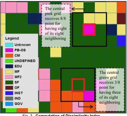
As Figure 3 shows, dissimilarity index is used to measure a 3-by-3 grid. In the top pink central cell case, if there are six neighboring cells (out of eight) with land uses that are different from the pink central cell, then the pink central cell gets 6/8 points. Following the same reasoning, the bottom green central cell outlined by the red frame is allocated 3/8 points because only three neighboring cells have different land uses.
Similar to entropy index, dissimilarity index also ranges from 0 to 1. The higher the value of dissimilarity index represents, the higher the variability of land uses. However, because it uses finer-grained cells (raster data format) rather than parcel lots (vector data format) as the unit of analysis, dissimilarity index is believed to present more accurate information about the type or intensity of mixing compared to entropy index.
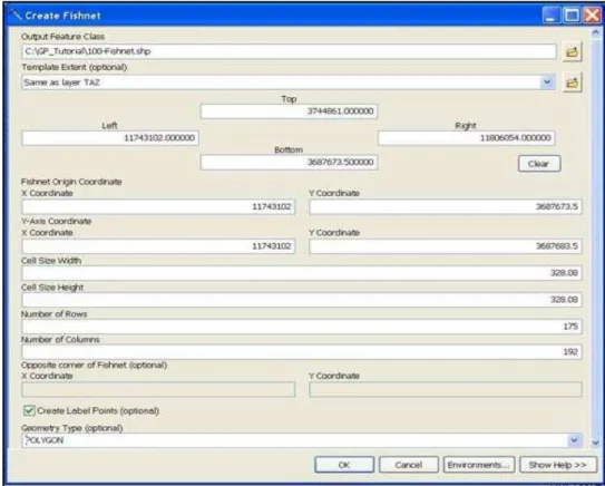
Computing Procedures of Dissimilarity Index. Create a Fishnet with 100 Meters ×100 Meters Grid Cells. While the vector data of land use parcel is used in computing entropy index, the hectare grid cell is used as the unit of analysis in computing dissimilarity index. Therefore, a layer of hectare grid cells is needed to cover the entire study area.
First, a fishnet is created using one ArcGIS tool: Arc Toolbox/Data Management Tool/Feature
Class/Create Fishnet. The fishnet consists of 100 meters ×100 meters grid cells (i.e., 328.08 feet × 328.08 feet shown in Figure 4). The net of 100 meters ×100 meters grid cells is a feature
The central
pink grid
receives 8/8
point for
having eight
of its eight
neighboring
The central
green grid
receives 3/8
point for
having three
of its eight
neighboring
class (vector data format), which resembles a fishnet. Therefore, every polygon formed by the
100 meters ×100 meters grid cell has its own object ID (OID) and spatial attributes.
Second, an additional ID field named “Uni_ID” is inserted in the fishnet layer in order to identify
each grid cell. Although every object in the feature layer already has an OID, a subsequent spatial join2) process between two objects may alter the OID number. To avoid this situation, an
additional ID field “Uni_ID” is inserted with the value copied from OID field. The fishnet layer of 100 meters ×100 meters grid cells is termed “100-Fishnet.”
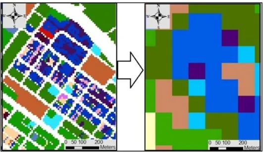
Rasterization of Land Use Layer. This step involves converting the vector layer of existing land-use to a raster layer for mapping grid cells. The ArcGIS tool is: Arc Toolbox/Conversion Tools/
To Raster/Feature to Raster. The output cell size is 10 meters ×10 meters, so it can be
integrated into the 100-Fishnet layer. See Figures 5 and 6 for details.
The 100-Fishnet is a vector layer, but the 10 meters ×10 meters grid of cells is a raster layer. Since a raster layer does not contain an OID for each grid cell, which is required for calculating dissimilarity index, it is necessary to eventually create a vector layer to replace the raster
layer’s attributes.
Fig. 4 –Creation of Fishnet
Transfer of the land-use information to 100-Fishnet and Conversion of Its Format from Raster Layer into Vector Layer. This step first encodes the land-use information from 10 meters × 10 meters grid-cells (raster layer) to 100-Fishnet (vector layer).
The Arc Toolbox/Spatial Analyst Tools/Zonal/Zonal Statistics tool is used to calculate the major land-use type for each hectare. The major land-use type among the 10 meters × 10 meters grid
cells is chosen for each 100 meters × 100 meters grid cell (Zone).
However, the new output layer is still in raster format. The 100 meters × 100 meters grid is just a frame that allows the raster layer (10 meters × 10 meters grid) to have the same spatial
layout as the 100-Fishnet layer. Figure 7 shows how this process works.
Fig. 5 - Rasterize Land Use Layer Fig. 6 – Raster Attribute Table
The last step is to convert the new raster layer to a vector layer using the polygon method. The ArcGIS tool is: Arc Toolbox/Conversion Tool/From Raster/Raster to Polygon. In this case, the
new polygon (vector) layer is termed “Raster-Polygon.”
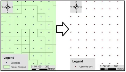
Identify Each 100 Meters * 100 Meters Grid Cell. Each grid cell of the raster-polygon layer (vector) is assigned a unique ID number imported from the 100-Fishnet layer. A centroid layer is created and assigned the input feature layer as the layout of the 100-Fishnet. This action creates a centroid layer with the same layout features as the 100-Fishnet. For example, the 100-Fishnet layer is 192×175 grid cells. Therefore, the centroid layer should also have
192×175 (33,600) points.
Figure 8 illustrates how these two layers are combined to form a point-feature layer. The ArcGIS tool is: Arc Toolbox/XTools/Feature Conversions/Shapes to Centroids. The
raster-polygon layer is then “spatial joined” (Arc Toolbox/Analysis Tool/Overlay/Spatial Join) to the
centroids layer. Hence, the new output layer with a centroid feature is shown with information from the raster-polygon layer. The new output centroid layer in this case is called “Centroid
-SP1.”
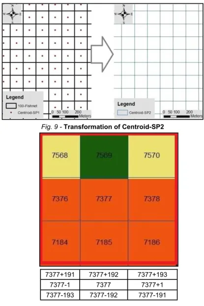
The Centroid-
SP1 layer undergoes another “spatial join” with 100
-Fishnet, as shown
in Figure 9. The new output feature is a 100-
Fishnet, called “Centroid
-
SP2.” In this
final layer, each Centroid-SP2 grid cell is encoded with the dominant land-use
category.
Dissimilarity Index Calculation
Dissimilarity index is produced in Microsoft Excel because of its complex calculation requirements. After exporting the Centroid-SP2 attribute table to Excel, unnecessary fields will
be deleted, leaving only the fields of “Uni_ID” and “Land Use Code (LU Code).” Recall that the
index formula is ∑jk∑18 (Xi/8)]/K. The “Uni_ID” data represents each grid cell and the Xi. Each ID has a specific pattern, shown in Figure 10, which is an arithmetic progression, based on the
values of the neighboring cells. The difference of 192 is from the number of columns in the 100-Fishnet layer.
As a result, this part of dissimilarity index (∑18 (Xi/8)) can be written using the Excel VLOOKUP3) function, as follows:
∑18 (Xi/8)=SUM(IF(B7378=(VLOOKUP(A7377-193,$A$2:$B$33601,2,FALSE)),0,1), IF(B7377=(VLOOKUP(A7377-192,$A$2:$B$33601,2,FALSE)),0,1),
Fig. 9 - Transformation of Centroid-SP2
7377+191 7377+192 7377+193
7377-1 7377 7377+1
7377-193 7377-192 7377-191
Fig. 10 -Pattern of the Cell Numbers
IF(B7377=(VLOOKUP(A7377-191,$A$2:$B$33601,2,FALSE)),0,1), IF(B7377=(VLOOKUP(A7377-1,$A$2:$B$33601,2,FALSE)),0,1), IF(B7377=(VLOOKUP(A7377+1,$A$2:$B$33601,2,FALSE)),0,1), IF(B7377=(VLOOKUP(A7377+193,$A$2:$B$33601,2,FALSE)),0,1), IF(B7377=(VLOOKUP(A7377+192,$A$2:$B$33601,2,FALSE)),0,1), IF(B7377=(VLOOKUP(A7377+191,$A$2:$B$33601,2,FALSE)),0,1))/8
The next step is to calculate K (the number of developed grid-cells in the TAZ). The Pivot Table tool in Excel is used to calculate the count of Uni_ID and the sum of dissimilarity index for each
TAZ. To complete the index computation, the “sum of dissimilarity” is divided by the “count of Uni_ID.” All the index results are between 0 and 1.
Statistical Analysis
The statistical analysis portion of this paper consists of two components.
The first component is the correlation analysis among home-based trip rates, land-use mixture indices (entropy and dissimilarity), and socioeconomic variables. This will reveal the one-on-one relationship between each pair of variables.
The second component is the multivariate regression analysis, which shows the combined effects of multiple independent variables (predictors) on a dependent variable (in this case, it is home-based work trip rate and home-based other trip rate). The independent variables not only include entropy and dissimilarity indices, which measure land-use mixture, but also additional socioeconomic variables [population/acre, auto/acre, population/household (HH), auto/ household (HH)]. In this way, the regression results will help determine whether land-use mixture variables or socioeconomic density variables at traffic analysis zone level and household level have larger effects on home-based trip making.
Since this study is a cross-sectional analysis using traffic analysis zone (TAZ) as a basic unit of analysis, it cannot definitively answer the causality question.
Richmond, Virginia: An Overview
Geographic Location
Figure 11 shows Richmond City (red colored) and its surrounding counties. Located approximately 100 miles south of Washington D.C., Richmond City is the capital city of the Commonwealth of Virginia, adjoining Henrico County and Chesterfield County.
Demography
In the year 2011, Richmond City had 201,828 residents and 166,384 employees. There were 93,837 workers living in the city and 160,603 workers working in the city. The daytime population was 268,594 people, calculated as: Total resident population + Total workers working in area - Total workers living in area. Therefore, the employment residence ratio was as low as 1.71 (Total workers working in the area / Total workers living in the area) (Source: American FactFinder 2011).
clustered around CBD. As shown in Figure 12, the Fan District west of the downtown area has the highest population density.
Fig. 11 -
Richmond City and Its Surrounding
Counties
Fig. 12
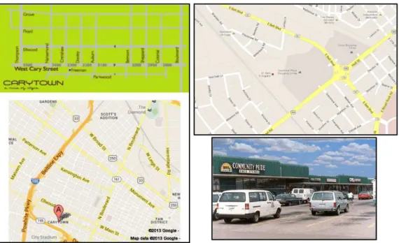
According to the Richmond Strategic Multimodal Transportation Plan, the densest employment area is within the CBD. That plan also indicates that the retail areas of Carytown (Note: Carytown is an urban retail district lining Cary Street at the southern end of the Museum District in Richmond, Virginia.The district includes over 300 shops, restaurants, and offices.), Southside Plaza [Note: Southside Plaza is a strip mall on Richmond's south side (south of the James River). Its principal tenants are Farmer's Foods and CVS drug & pharmacy among smaller stores.], and the fragmented industrial areas located south of the James River all contain sites that provide a relatively large number of jobs, with the employment density of more than 10 jobs per acre (Source: http://www.yesrichmondva.com/transportation-development/Richmond-Strategic-Multi-Modal-Transportation). See Figure 13 for Carytown and Southside Plaza.
Land Use
The types of general land-use impact the pattern of local travel behavior. The land in the CBD has various uses, the majority of which are commercial and official uses. Throughout the city, the commercial land uses are located along several primary streets and areas, such as West and East Broad Streets, and the area within Belvidere Boulevard (a major street linking Chamberlayne Avenue and Jefferson Davis Highway, unlabeled in Figure 14) and, I-95, I-64, and I-195. South of the city, the commercial functions are found linearly along Midlothian Turnpike, Hull Street, and Jefferson Davis Highway.
Outside of the downtown (commercial and official land uses) and the southeast area (industrial land uses), single-family residential housing comprises the majority of the total developed land,
up to 41.8% within the city’s walking and bicycle paths.
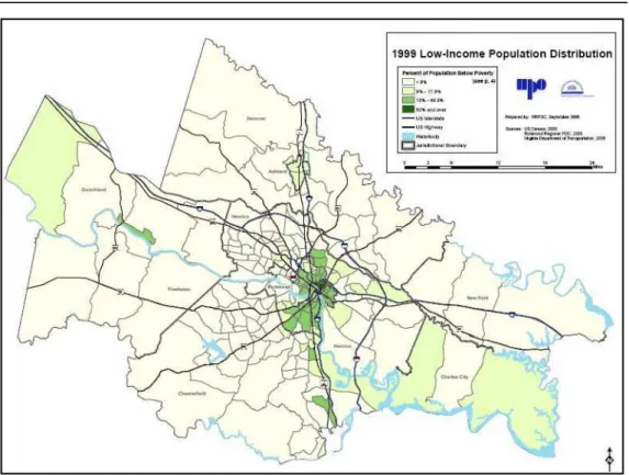
Poverty
Figure 15 shows the 1999 low-income population distribution in the Richmond metropolitan area, which contains Richmond City as the central city. It clearly shows that the poorest areas are concentrated in and near CBD area, including North Side, East End, and South Side.
The urban fringe areas and suburban counties had much lower percent of population under poverty. This pattern is consistent with that of the other metropolitan areas in the country.
Transportation
The James River runs through the center of the city. Interstates 95 and 64 intersect in the downtown area, and Interstate 195 and Virginia State Route 288 separately encircle the east and west sides of the city.
Like in the rest of the U.S., automobile is the principal transportation means for the Richmond residents. Table 2 shows the modeled 2008 modal shares for the total daily trips occurring in the entire Richmond/Tri-Cities Model Region, which includes the following list of jurisdictions: Chesterfield, Colonial Heights, Hanover, Henrico, Hopewell, Richmond, Petersburg, Charles City (partial), Dinwiddie (partial), Goochland (partial), New Kent (partial), Powhatan (partial), Prince George (partial). Figure 16 shows the Richmond/Tri-Cities Model Region. The entire Model Region currently has about 1.2 million population, about six times as large as its central
city’s population. According to the model estimate, automobiles had more than 98% of the total
regional modal share.
However, for Richmond City, the modal share is very different from that of the region, with a much higher transit modal share for its commuting workers (7%). According to the 2007-2011 American Community Survey 5-Year Estimates, Richmond City had the following modal shares for its commuting workers 16 years and over (total number is 94,373). See Table 3 for details.
When comparing Table 2 and Table 3, it should be noted that central city should have a much higher transit modal share than its suburban counterpart. In addition, commuting workers should also have much higher transit modal shares than general population. Therefore, there exists a huge discrepancy of transit modal share between the modeled Table 2 and observed Table 3.
Table 2
2008 Regional Modal Shares
Trip Purpose Total Person Trips
Auto Person Trips Transit Person Trips
Number of
Trips Percent
Number of
Trips Percent
All 3,184,052 3,139,666 98.6 44,386 1.4
Peak 539,809 527,721 97.8 12,088 2.2
Off-Peak 2,644,243 2,611,945 98.8 32,298 1.2
Home-Based Work
719,646 702,100 97.6 17,546 2.4
Peak 258,784 250,439 96.8 8,345 3.2
Off-Peak 460,862 451,661 98.0 9,201 2.0
Home-Based Other
1,790,111 1,767,430 98.7 22,680 1.3
Peak 214,338 211,101 98.5 3,238 1.5
Off-Peak 1,575,772 1,556,329 98.8 19,443 1.2
N o n - H o m e Based
674,296 670,135 99.4 4,160 0.6
Peak 66,687 66,181 99.2 506 0.8
Off-Peak 607,608 603,954 99.4 3,654 0.6
Source: Virginia Department of Transportation. (2008), Richmond/Tri-Cities Transportation Model. No
Table 3
Modal Shares of Richmond Commuting Workers
Modes Number of Trips Percent
Car, truck, or van -- drove alone 66,614 70.6%
Car, truck, or van -- carpooled 10,980 11.6%
Public transportation (excluding taxicab) 6,568 7.0%
Walked 4,171 4.4%
Other means 2,689 2.8%
Worked at home 3,351 3.6%
In the Richmond region, the principal transit operator is the Greater Richmond Transit Company (GRTC), which primarily serves Richmond City. As illustrated in Figure 17, the GRTC bus stops and routes are concentrated in the northern part of the city, i.e. north of the James River (crossing the city in the central area and blue colored), especially in the downtown area. The northern part of Richmond has a better accessibility to public transportation facilities as the 0.25-mile buffer zones of the GRTC bus routes cover most of the area.
Figure 18 shows the distribution of based work trip rate for the city. The highest home-based work trip rates are found in a small block of the CBD, north of Broad Street, and southeast of the intersection of I-95/I-64 and I-195. The second highest rates of home-based work trips are found mostly in the residential, industrial, or commercial areas of Richmond, such as the Far West neighborhood, a partial area of the Broad Rock neighborhood between
the Jefferson Davis Highway and Midlothian Turnpike, the Woodland Heights neighborhood, etc.
Figure 19 shows that the home-based other trips are mostly generated to the north of Broad Street, or the area between the Jefferson Davis Highway and Midlothian Turnpike. The highest home-based other trip rates are found between 7th and 12th Streets within the CBD.
Results of Analysis
This section documents and analyzes the results of computing both entropy and dissimilarity indices, and conducting correlation / regression analysis among these two indices, socioeconomic variables, and home-based trip making.
This paper uses traffic analysis zone (TAZ) in the Richmond/Tri-Cities Model as a basic unit of
analysis. The computing process is also called “NEAT-GIS” (Neighborhood Environment for Active Transport –Geographic Information Systems) (D’Sousa et al. 2010). While GIS handles the geographic analysis portion of the work, calculation of the indices will be completed using Microsoft Excel. Following the computing procedures described in the Methodology Section, the results are shown below.
Entropy Index of the Richmond Land Use Mixture
Figure 20 uses a darker red color to indicate higher entropy and higher heterogeneity of land uses. It indicates that the areas with the highest mixing level or entropy value over 0.90 are located in the CBD between 7th and 9th Streets. The other areas with the high level of land-use mixture are located near the intersection of I-195 and Broad Street, and the southwest part of the City near the intersection of Forest Hill Avenue and Route-76 (Powhite Parkway). The lowest entropy areas are located in the southwest of Monument Avenue and I-195 (Downtown Expressway) with an entropy value under 0.2, where single-family residential land uses are dominant.
Dissimilarity Index of the Richmond Land Use Mixture
As illustrated in Figure 21, by using dissimilarity index as an indicator of land-use mixture, the mixed land use areas are even more clustered in the downtown area of Richmond than by
using entropy index as an indicator. In addition to downtown area, the Fan District has a very high level of land-use mixture.
In summary, whether using entropy index and dissimilarity index, downtown, nearby areas along Broad Street, and a few major street intersections have a relatively high level of land-use mixture. The outlying areas, especially residential areas, are more homogeneous with low level of land-use mixture.
Correlation Analysis between Home-Based Trip Rates and Land-Use Mixture Indices
This section first generates scatterplots (Fig. 22) and then conducts a correlation analysis between home-based trip rates (home-based work and home-based other) and land-use mixture indices (entropy and dissimilarity). The correlation matrix is shown in Table 4.
From Figure 22, it can easily be seen that home-based work trip rate, shown as a downward sloping line, is slightly inversely proportional to entropy and dissimilarity indices. However, home-based other trip rate, shown as a straight line, is almost completely independent of entropy and dissimilarity indices.
As shown in Table 4, entropy index and dissimilarity index are highly correlated (.700). This suggests that these two indices point to the generally same direction in measuring land-use mixture.
Table 4 indicates that home-based work trip rates are negatively correlated with either entropy
index or dissimilarity index, with the Pearson correlation coefficient (r) to be -.145 and -.205, respectively. This indicates that, with an increase in degree of land-use mixture (larger entropy and dissimilarity indices), there will be a decrease in home-based work trip rates, even though the correlation strength is relatively weak. That dissimilarity index is relatively more correlated with home-based work trip rates than entropy index suggests that dissimilarity index may be a better indicator to measure land-use mixture than entropy index.
Mixed land uses tend to induce more walking, cycling, or transit trips. Transit trips typically serve home-based work trip purpose occurring during peak periods. Because of this reason, land-use mixture seems to have a somewhat positive effect on the reduction of home-based
work trips. This statistical analytical result corroborates Cervero’s finding that although land-use mixture has a correlation to commuting, its correlation strength is not very strong (Cervero 1996).
In the meantime, home-base other trips can take place at any time. Because of this reason, land-use mixture has very limited or negligible impacts on home-based other trip rates.
Correlation Analysis between Home-Based Trip Rates and Socioeconomic Variables
Cervero further argues that, besides land-use mixture, neighborhood density and automobile availability are the main factors influencing the commuting choice of residents (Cervero 1996).
Table 4
In another paper, Chen and Suen (2010) indicated that, in Richmond, socioeconomic variables have larger impacts on travel making and mode choices than land use variables. To test the validity of both arguments, this section will conduct additional correlation analysis between home-based trip rates and zonal/household socioeconomic variables.
Due to the data limitation, only two trip production-sided socioeconomic variables are used: population and auto. For zonal analysis, two density-related variables are calculated: population/acre and auto/acre. For household analysis, two household-related variables are calculated: population/HH and autos/HH. Therefore, zonal analysis uses acres as an areal unit, whereas household analysis uses household as unit. Figures 23 and 24 show that household-related variables, especially auto per household, are more closely household-related to home-based trip rates than zonal density-related variables.
Table 5 is the correlation matrix between home-based trip rates and zonal socioeconomic variables. It clearly indicates that home-based trip rates and zonal socioeconomic variables are
Table 5
Correlation Matrix between Home-Based Trip Rates and Zonal Socioeconomic Variables
Table 6
largely independent of each other with very low and negligible correlation. This means that the socioeconomic variables in surrounding areas have very little effects on home-based trip making behaviors.
Table 6 is the correlation matrix between home-based trip rates and household socioeconomic variables. This table presents the opposite results from those of Table 5. It is particularly worth noting that autos/HH is highly correlated with home-based work trip rates (.552) and home-based other trip rates (.557).
Regression Analysis of Home-Based Work Trip Rates
In this analysis, the following variables are assumed:
Dependent variable = home-based work trip rate; and
Independent variables = Entropy index, Dissimilarity index, Population/Acre, Auto/Acre, Population/HH, Auto/HH.
The multivariate regression results are shown in Table 7. The entire model performs well with a good R2 value (.522). ANOVA results also confirm that the model is significant with a large F value.
In terms of contributions from independent variables (predictors), Auto/HH is apparently the most significant variable impacting home-based work trip rate with the highest t value (11.189). Both Entropy index and Dissimilarity index are negatively related to home-based work trip rate, but Dissimilarity index is much more significant than Entropy index in impacting home-based work trip rate. Entropy index is actually insignificant with a very small t value (-.260).
These findings from the regression analysis are consistent with those from the correlation analysis.
Regression Analysis of Home-Based Other Trip Rates
With respect to the analysis on home-based other trip rate, the following variables are assumed:
Dependent variable = home-based other trip rate; and
Independent variables = Entropy index, Dissimilarity index, Population/Acre, Auto/Acre, Population/HH, Auto/HH. The multivariate regression results are shown in Table 8.
Like home-based work trip rate model, the entire model for home-based other trip rate performs well with a good R2 value (.459). ANOVA results also confirm that the model is significant with a large F value.
In terms of contributions from independent variables (predictors), Auto/HH is still the most significant variable impacting home-based other trip rate with a high t value of 10.366. However, both Entropy index and Dissimilarity index are insignificant with very small t values (.490 and .873, respectively).
Table 7
Conclusion
Through this empirical study of Richmond, Virginia, it has been found that:
First, land-use mixture has some but not strong positive effects on home-based work trip rate, but has virtually no or negligible effects on home-based other trip rate.
Table 8
Second, socioeconomic characteristics in larger surrounding areas have very little effects on home-based trip making.
Third, household socioeconomic characteristics have direct and positive effects on based trip making, especially auto ownership variable, which is positively related to home-based trip rate.
Fourth, both correlation analysis and regression analysis have yielded the generally consistent findings.
In conclusion, the link between home-based trip making and land-use mixture is still far from clear, requiring more in-depth and detailed analysis at different geographic scales. Compared to land use variables, socioeconomic variables seem to have more direct effects on home-based trip making.
References
BADOE, D., A., MILLER, E., J. (2000), Transportation-land-use interaction: empirical findings in North America, and their implications for modelling, Transportation Research Part D, 5, 4, pp. 235–263.
BHAT, C., R., ELURU, N. (2009), A Copula-based approach to accommodate residential self-selection effects in travel behavior modelling, Transportation Research B, 43, 7, pp. 749–765.
BOARNET, M., G. (2011), A Broader Context for Land Use and Travel Behavior, and a Research Agenda, Journal of the American Planning Association, 77, 3, pp. 197-213.
BOARNET, M. G., AND CRANE, R. (2001), Travel by design: The influence of urban form on travel, Oxford University Press.
BOARNET, M., G., SARMIENTO, S. (1998), Can land use policy really affect travel behaviour ?, Urban Studies, 35, 7, pp. 1155–1169.
BROWNSTONE, D. (2008), Key relationships between the built environment and VMT,
Draft paper prepared for the Transportation Research Board panel, “Relationships Among Development Patterns, Vehicle Miles Traveled and Energy.”
BRUEGMANN, R. (June 18, 2007), Brawl Over Sprawl, Los Angeles Times. Retrieved April 9, 2012.
CALTHORPE, P. (1993), The next American metropolis: Ecology, community, and the American dream, Princeton Architectural Press.
CAO, X. (2010), Exploring causal effects of neighborhood type on walking behavior using stratification on the propensity score, Environment and Planning A, 42, 2, pp. 487–504.
CAO, X., MOKHTARIAN, P., L., HANDY, S., L. (2009), Examining the impacts of residential self-selection on travel behaviour: A focus on empirical findings, Transport Reviews,
29, 3, pp. 359–395.
CAO, X., XU, Z., FAN, Y. (2009), Exploring the connections among residential location, self-selection, and driving behavior: A case study of Raleigh, NC, Paper presented at the 89th annual meeting of the Transportation Research Board.
CERVERO, R. (1986), Suburban Gridlock, New Brunswick, NJ Centre for Urban Policy Research Press.
CERVERO, R. (1989), Jobs-housing balancing and regional mobility, Journal of the American Planning Association, 55, 2, pp. 136-150.
CERVERO, R., DUNCAN, M. (2006), Which Reduces Vehicle Travel More: Jobs-Housing Balance or Retail-Jobs-Housing Mixing?, Journal of the American Planning Association, 72, 4, pp. 475-490.
CERVERO, R., KOCKELMAN, K. (1996), Travel demand and the three Ds: density, diversity, and design, Working Paper No. 674, Institute of Urban and Regional Development, University ofCalifornia, Berkeley.
CERVERO, R., KOCKELMAN, K. (1997), Travel demand and the 3 Ds: Density, diversity and design, Transportation Research Part D, 2 (3), pp. 199–219.
CHEN, X., SUEN, I.-S. (2010), Richmond's Journey-To-Work Transit Trip-Making Analysis, Management Research And Practice, 2, 3, pp. 234-248.
COX, W., UTT, J. (June 25, 2004), The Costs of Sprawl Reconsidered: What the Data Really Show, Heritage Foundation Backgrounder #1770, The Heritage Foundation.
CRANE, R. (2000), The influence of urban form on travel: An interpretive Review, Journal of Planning Literature, 15, 1, pp. 3–23.
CRANE, R., CREPEAU, R. (1998), Does neighborhood design influence travel? A behavioral analysis of travel diary and GIS data, Transportation Research Part D, 3, 4, pp. 225
–238.
D’SOUSA, E. et al. (2010), Environment and Physical Activity GIS Protocols Manual, in:
(A. Forsyth, Ed.). Design for Health. Retrieved November 1, 2011 from: http:// www.designforhealth.net/resources/gis_protocols.html.
DUANY, A., PLATER-ZYBERK, E. (1991), Towns and town-making Principles, Rizzoli. EWING, R., CERVERO, R. (2001), Travel and the built environment: A Synthesis, Transportation Research Record, 1780, pp. 87–114.
EWING, R., CERVERO, R. (2010), Travel and the built environment: A meta-analysis, Journal of the American Planning Association, 76, 3, pp. 265–294.
EWING, R., HALIYUR, P., PAGE, G., W. (1995), Getting around a traditional city, a suburban planned unit development, and everything in between, Transportation Research Record, 1466, pp. 53–62.
FRANK, L., PIVO, G. (1995), Impacts of mixed use and density on utilization of three modes of travel: Single-occupant vehicle, transit, and walking, Transportation Research Record, 1466, pp. 44–52.
FRIEDMAN, B., GORDON, S., P., PEERS, J., B. (1994), Effect of neotraditional neighborhood design on travel characteristics, Transportation Research Record, 1466, pp. 63-70.
GORDON, P., RICHARDSON, H., W. (2001), The Geography of Transportation and Land Use, In: Holcombe, R. G. and S.R. Staley (Eds.). Smarter Growth: Market-Based Strategies for Land-Use Planning in the 21st Century, Greenwood Press.
HANDY, S., L. (2005), Smart growth and the transportation–land use connection: What does the research tell us?, International Regional Science Review, 28, 2, pp. 146–167.
HANDY, S., L., CAO, X., MOKHTARIAN, P., L. (2005), Correlation or causality between the built environment and travel behaviour ? Evidence from Northern California, Transportation Research Part D, 10, 6, pp. 427–444.
HEATH, G., W., BROWNSON, R., C., KRUGER, J., MILES, R., POWELL, K., E., RAMSEY, L., T. (2006), The effectiveness of urban design and land use and transport policies and practices to increase physical activity: A systematic review, Journal of Physical Activity and Health, 3, 1, pp. S55–S76.
HENDERSON, K., A., BIALESCHKI, M., D. (2005), Leisure and active lifestyles: Research reflections, Leisure Sciences, 27, 5, pp. 355–365.
KELBAUGH, D., S. (Ed.) (1989), The pedestrian pocket book: A new suburban design strategy, Princeton Architectural Press.
neighborhood-scale urban form matter?, Journal of The American Planning Association, 69, 3, pp. 265–281.
KUZMYAK, R., J., PRATT, R., H. (2003), Land Use and Site Design: Traveler Response to Transport System Changes, Chapter 15, Transit Cooperative Research Program Report 95, Transportation Research Board (www.trb.org). Retrieved June 2013 from: http://gulliver.trb.org/ publications/tcrp/tcrp_rpt_95c15.pdf.
LITMAN, T., STEELE, R. (2012), Land Use Impacts on Transport How Land Use Factors Affect Travel Behavior. Retrieved June 7, 2013 from: http://www.vtpi.org/landtravel.pdf.
MCFADDEN, D. (2007), The behavioral science of transportation, Transport Policy, 14, 4, pp. 269-274.
MCNALLY, M., G., KULKARNI, A. (1997), Assessment of the land-use-transportation system and travel behavior, Transportation Research Record, 1607, pp. 105-115.
MODARRES, A. (1993), Evaluating Employer-Based Transportation Demand Management Programs, Transportation Research Record A, 27, 4, pp. 291-297.
MOKHTARIAN, P., L., CAO, X. (2008), Examining the impacts of residential self-selection on travel behavior: A focus on methodologies, Transportation Research B, 43, 3, pp. 204–228.
SALON, D. (2006), Cars and the City: An Investigation of Transportation and Residential Location Choices in New York City, Dissertation submitted in fulfillment of the Ph.D.
in Agricultural andResource Economics, University of California, Davis.
SARZYNSKI, A., WOLMAN, H., L., GALSTER, G., HANSON, R. (2006), Testing the Conventional Wisdom about Land Use and Traffic Congestion: The More We Sprawl, the Less We Move?, Urban Studies, 43, 3, pp. 601-626.
SPEARS, S., BOARNET, M., G., HANDY, S., L. (2010), Draft policy brief on the impacts of land use mix based on a review of the empirical literature, California Air Resources Board, Retrieved May 23, 2011, from http://arb.ca.gov/cc/sb375/policies/policies.htm.
STEAD, D. (2001), Relationships between land use, socioeconomic factors, and travel patterns in Britain, Environment & Planning B: Planning & Design, 28, 4, pp. 499-528.
THILL, J., C., KIM, M. (2005), Trip making, induced travel demand, and accessibility, Journal of Geographical Systems, 7, 2, pp. 229-248.
TRANSPORTATION RESEARCH BOARD (2011), Enhancing Internal Trip Capture Estimation for Mixed-Use Developments, National Cooperative Highway Research Program (NCHRP) Report 684.
ZHOU, B., KOCKELMAN, K. (2008), Self-selection in home choice: Use of treatment effects in evaluating the relationship between the built environment and travel behaviour, Transportation Research Record, 2077, pp. 54–61.
Initial submission: 1.04.2013 Revised submission: 9.06.2013 Final acceptance: 12.06.2013
Correspondence: Xueming Chen, Rm. 511, Scherer Hall, 923 West Franklin Street, Richmond, VA 23284-2028, P: (804) 828 -1254 / F: (804) 827 – 1275.