From cognitive science to management science: two computational contributions

daniel de magalhães chada

F R O M C O G N I T I V E S C I E N C E T O M A N A G E M E N T S C I E N C E : T W O C O M P U TAT I O N A L

Escola Brasileira de Administração Pública e de Empresas

-EBAPE

Fundação Getulio Vargas

F R O M C O G N I T I V E S C I E N C E T O

M A N A G E M E N T S C I E N C E : T W O

C O M P U TAT I O N A L C O N T R I B U T I O N S

daniel de magalhães chada

B.Sc. Pontifícia Universidade Católica do Rio de Janeiro,

2007

Dissertação submetida como requisito para a obtenção do

grau

Mestre de Administração

banca examinadora:

Alexandre Linhares (Orientador - EBAPE-FGV) Horácio Hideki Yanasse (INPE)

Rafael Guilherme Burstein Goldszmidt (EBAPE-FGV)

local: Rio de Janeiro data: Maio2011

From Cognitive Science to Management Science: Two Computational Contributions ©

copyright byDaniel de Magalhães Chada 2011

Ohanameans family.

Family means nobody gets left behind, or forgotten.

— Lilo & Stitch

Dedicated to the loving memory of Edson de Campos Chada.

A B S T R A C T

This work is composed of two contributions. One borrows from the work of Charles Kemp and Joshua Tenenbaum, concerning the dis-covery of structural form: their model is used to study the Business Week Rankings of U.S. Business Schools, and to investigate how other structural forms (structured visualizations) of the same information used to generate the rankings can bring insights into the space of business schools in the U.S., and into rankings in general. The other essay is purely theoretical in nature. It is a study to develop a model of human memory that does not exceed our (human) psychological short-term memory limitations. This study is based on Pentti Kanerva’s Sparse Distributed Memory, in which human memories are registered into a vast (but virtual) memory space, and this registration occurs in massively parallel and distributed fashion, in ideal neurons.

R E S U M O

Este trabalho é composto de duas contribuições. Uma se usa do tra-balho de Charles Kemp e Joshua Tenenbaum sobre a descoberta da forma estrutural: o seu modelo é usado para estudar osrankings da revista Business Week sobre escolas de administração, e para investigar como outras formas estruturais (visualizações estruturadas) da mesma informação usada para gerar osrankingspode trazer discernimento no espaço de escolas de negócios nos Estados Unidos e emrankingsem geral. O outro ensaio é de natureza puramente teórica. Ele é um estudo no desenvolvimento de um modelo de memória que não excede os nossos (humanos) limites de memória de curto-prazo. Este estudo se baseia na Sparse Distributed Memory (Memória Esparsa e Distribuida) de Pentti Kanerva, na qual memórias humanas são registradas em um vasto (mas virtual) espaço, e este registro ocorre de forma maciçamente paralela e distribuida, em neurons ideais.

Gratitude bestows reverence, allowing us to encounter everyday epiphanies, those transcendent moments of awe that change forever how we experience life and the world. —John Milton (1608-1674)

A C K N O W L E D G M E N T S

Turns out this is the section upon which I put highest importance, but have the most trouble writing. I would like to thank my mother, Lúcia, whose tirelessness, hard work and dedication to her family are forever ingrained in my mind as the meaning of the word nobility. This work would not have been possible without her unwavering support.

I thank my future wife, Mariana, for her endless patience when I was frustrating, kindness when I was frustrated and support when ...always, actually.

I am unaware of how many advisees can honestly say they found great friends in their advisors, but I did in Alexandre Linhares. His capacity to shape an endless flow of raw creativity into highly original scientific work astounds me to this day. His support and optimism were undying when I convinced myself there were no results to be found, or when I found yetanotherbug in the software. I thank him for all this, and for making it all look easy and fun.

My uncle João Bosco and aunt Christina have been champions of my professional and academic development throughout my life, providing support when it was most needed. They are not my godfather and godmother by some twist-of-fate, but nonetheless hold places of honor and respect in my heart larger than any title can bestow.

I thank my colleagues-in-arms: Jarbas Silva, Ariston Diniz and more recently Marcelo Brogliato for countless enlightening conversations in our shared passion of science, computation and cognition.

And to Christian Aranha, my near-advisor through our years of work together: He brought me (almost dragged me, honestly) to the field to which I now hope to dedicate my career, and for that I will always be grateful.

I thank my fellow students at EBAPE/FGV for creating the won-derful atmosphere we shared throughout the course; and the staff at EBAPE/FGV for their professionalism and technical support.

I would also like to thank Eric Nichols for numerous valuable com-ments during the development of the SDM chapter.

C O N T E N T S

i introduction 1

1 cognition, decision and administration 3

ii form, structure and data 5

2 the multidimensional road to harvard or, why rank -ing business schools does not make sense 7

2.1 Introduction 7

2.1.1 Rank anomalies 8

2.1.2 The imposition of structure 10

2.2 On KT-Structures 11

2.2.1 Hierarchical Bayesian model: forms, structures,

and data 12

2.2.2 Graphs and graph grammars 13

2.2.3 Stirling Numbers 14

2.3 The Business Week2008Ranking 14

2.3.1 Materials and Methods 14

2.3.2 Numerical experiments 15

2.4 Summary 18

iii sparse distributed memory 21

3 the emergence of miller’s magic number on a sparse distributed memory 23

3.1 Introduction 23

3.1.1 Sparse Distributed Memory 24

3.1.2 Chunking through averaging 26

3.2 Analysis 27

3.2.1 Computing the Hamming distance from chunkα

to items 27

3.2.2 Varying the number of presented items 29

3.2.3 The chunking through averaging postulate 30

3.3 Discussion 31

iv conclusions and future work 35

4 conclusions 37

5 avenues of future exploration 39

v appendix 41

a apendix a: applying kt-structures: a tutorial for decision scientists 43

bibliography 45

L I S T O F F I G U R E S

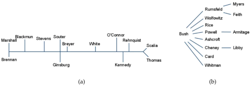
Figure1 Each of the four schools of Simplicia is related to two others by one—and only one—of their dimensions. 9 Figure2 (a) Spectrum extracted from justices’ votes; (b)

Hier-archy of the Bush cabinet 12

Figure3 (a) Tree-generative Graph Operation. (b) Cluster-generative Graph Operation 14

Figure4 The generated KT-Structure: an undirected hierarchy with no self-links. 17

Figure5 The KT-Structure distance between schools plotted against their ranked distance. 18

Figure6 Behavior at different dimensions and items presented 29

L I S T O F TA B L E S

Table1 Rank anomalies. Though schools ranked {22, 24,26, 27,28, and 29} seem close in the ranking, they are clearly separable into different clusters. 16 Table2 Thresholds TN,2σgiven plausible success factors and

dimension combinations. 28

A C R O N Y M S

KT Kemp-Tenenbaum

SDM Sparse Distributed Memory

API Application Programming Interface

Part I

1

One of the tenets of management science is to develop a comprehensive theory of human decision-making. While the rational-decision actor has been successful in modeling, and in bringing valuable insights into a number of decision scenarios, a number of studies have made clear that humans depart from rationality (for recent summaries, see [Smith e Winterfeldt2004,Ariely2008,Ariely2010]).

Cognitive science, the study of human information-processing, is slowly filling the void between the need for formal models of human behavior and the numerous shortcomings of the rational model. The computational tools generated through the field’s explorations into human behavior can provide new paradigms of pattern recognition, exploratory data analysis and information retrieval, all central to the aim of decision science.

For example, in the field of business strategy, [Gavetti et al.2005,

Gavetti e Warglien2007] postulate that choice, in novel environments at least, is guided by analogy-making. Case studies are a highly popular tool in business education and their value often hinges on the under-standing of one situation in terms of another. The literature provides a number of examples of analogical reasoning:

i) The chain "Toys ’R’ Us", launched in the1950s, was tied to the vision and success of supermarkets (the chain was effectively called "Baby Furniture and Toy Supermarket" at a particular point). Afterwards, the launch of the office store "Staples" was based on similar reasoning: "Could we create a Toys R Us for office supplies?" [Gavetti et al.2005]; ii) In the 1980s the largest European carmaker decided to invest heavily in the U.S. market by introducing a large range of cars that were bestsellers in Europe. Before this decision, the carmaker had63% of the imported car market in the U.S. But the carmaker was called Volkswagen. The American consumer’s experience with Volkswagen consisted of the Beetle, an inexpensive and odd-looking car first sold in 1938. American consumers rejected the idea of a large, well-built, modern-looking, powerful and expensive Volkswagen. To make matters worse, the company decided to withdraw the Beetle from the market, and its share of the imported car market in the U.S. dramatically fell from63% to less than4%. The exact same cars were being sold in Europe and in the U.S; the only difference was in the consumers’ experiences of what a "Volkswagen" meant. A twenty-thousand-dollar Volkswagen seemed, to Americans, like a practical joke. Similarly, "the new Honda" to an American consumer meant a new car model; to the Japanese, it meant a new motorcycle [Ries e Trout1993].

iii) When Iranian Ayatollah Ruhollah Khomeini declared a fatwa (a death sentence) to writer Salman Rushdie, the Catholic Church did not stand for the principle of "Thou shalt not kill". It recognized its experience of trying to censor "The last temptation of Christ", a film, and sided with the Iranians. L’Osservatore Romano, a key Vatican publication, condemned Rushdie’s book as ’blasphemous’. The Head of the French Congregation, Cardinal Decourtray, called it an ’insult to God’; Cardinal O’Connor from New York made it clear that it was

4 cognition, decision and administration

crucial to "let Moslems know we disapprove of attacks on their religion" [Hofstadter e FARG1995,Linhares e Freitas2010].

Decision-makers often obtain strategic insights by understanding one situation in terms of another; however, analogies are but one of the ideas from cognitive science that have crossed the bridge to manage-ment science. Neural Networks, or mathematical models of large-scale parallel processing in general, have found use in a number of more traditional management science domains, such as credit-risk evaluation [Piramuthu et al.1998], the understanding of new product develop-ment [Natter et al.2001], and consumer targeting [Kim et al.2005], to name a few.

This thesis constitutes two essays on cognitive science. One, in chapter 2, borrows from the work of Charles Kemp and Joshua Tenenbaum, concerning the discovery of structural form: Kemp and Tenenbaum’s model is used to study the BusinessWeek Rankings of U.S. Business Schools, and to investigate how other structural forms (structured visualizations) of the same information used to generate the rankings can bring insights into the space of business schools in the U.S., and into rankings in general.

The work of chapter2has an exploratory nature and is meant as a relevant incursion into a new concrete usage of cognitive modeling toward administrative practices. Its goal is to illustrate the inherent applicability of the discovery of structural form in exploratory data analysis.

The other essay, in chapter3, is purely theoretical. It is a study to de-velop a model of human memory that does not exceed our psychological short-term memory limitations. This study is based on Pentti Kanerva’s ’Sparse Distributed Memory’ (SDM) [Kanerva1988], in which human memories are registered into a vast (but virtual) memory space, and this registration occurs in massively parallel and distributed fashion, in idealized neurons [Linhares et al.2011].

Before we enter into further details, the reader may ask: why these two particular topics? Why the work of Kanerva; or the work of Kemp and Tenenbaum? The response to this question gives a glimpse of the history of this manuscript. In brief, a future model of the human mind, and thus of decision-making, must incorporate features relating these two bodies of work. Human memory has numerous psychological characteristics reflected in Sparse Distributed Memory, and it is possible that this model, or a variation of it, explains how we register information at the most basic level.

Additionally, humans are able to discover different forms in our surroundings, from a linear ordering of aggressive primates, to the self-clustering of prisoners, to the hierarchical trees representing power in the inner circles of the White House. In other words, we are able to perceive not only relationships between entities, but also that these relationships are classifiable into different forms.

Part II

2

O R , W H Y R A N K I N G B U S I N E S S S C H O O L S D O E S N O T M A K E S E N S E

Science is facts; just as houses are made of stones, so is science made of facts; but a pile of stones is not a house and a collection of facts is not necessarily science. — Henri Poincaré (1854-1912)

2.1 introduction

Business schools are regularly ranked by Business Week, The Economist, US News & World Report, Fortune, Financial Times, the Wall Street Journal, amongst many other organizations and periodicals. Their publication, beginning in the1980s, have generated high controversy in the U.S. and abroad. These rankings exert deep influence across the business school landscape [Pfeffer e Fong2004, Gioia et al.2000,

Gioia e Corley2002,Corley e Gioia2000,Alvesson1990]. They directly affect the perceptions of current students, alumni and prospective stu-dents in regards to the quality of the ranked schools. Their influence has repercussions to the extent that schools alter their curricula, fire faculty, and adapt teaching methods with the explicit objective of ris-ing in the ranks. Zell [Zell2001] elaborates on this change of behav-ior since the rise of the business school rankings. Pfeffer and Fong [Pfeffer e Fong2004] explain how i) business schools taylor their cur-ricula in attempts to rise on the ranking; ii) professors "dumb down" their courses in order to receive better reviews from students; iii) the press (rather than academia) has led the way in defining standards of world-class business education and iv) the above points cause a stan-dardization of business schools, which is detrimental to students (who lose options for different types of education) and to schools. Corley and Gioia [Corley e Gioia2000] explain how “the rankings by these mag-azines have come to dominate many business schools’ sense-making and action-taking efforts”.

Dichev [Dichev1999] questions the validity of rankings as a whole, concluding from a cross-rankings correlation that neither the Business Week nor the U.S. News rankings “should be interpreted as a broad measure of school quality and performance”, and that the “absence of positive correlation combined with reversibility in changes implies that one should avoid a broad interpretation of the rankings as measures of the unobservable ’school quality”’. Still others suggest alternate evaluation methods for schools, using different indicators to provide a ’better’ ranking system [Tracy e Waldfogel1997] or better principles [Cornelissen e Thorpe2002] in order to better reflect the qualities of each institution. (These, nevertheless, also impose the order structure, which is the critical point of focus here.)

While students and alumni generally regard the rankings as a valid metric of the quality and reputation of the schools, faculty and staff generally share a more adverse view of this system. Among the latter, they are viewed as poor quality indicators of the education provided

8 the multidimensional road to harvard or, why ranking business schools does not

by an institution. Furthermore, studies show that there is virtually no correlation between a position in the ranking and academic production [Siemens et al.2005, Trieschmann et al.2000]. Other evidence shows that both the rankings themselves [Elsbach e Kramer1996] and the changes caused by them [Pfeffer e Fong2004,Zell2001] elicit responses ranging from mild annoyance to outright rebelliousness amongst fac-ulty. As a testament to the power and influence of rankings, there is empirical evidence showing the correlation between the rankings and the resignations of the deans of schools that score poorly on them [Fee et al.2005]. From this body of literature one may conclude that rankings hold a huge sway over institutions and their strategies—and over the students’ choices concerning which one to attend—despite their clear dissociation from any true measure of the quality of the education at each institution. Similar discussions arise from university– level rankings [Ehrenberg et al.2001, Liu e Cheng2005, Florian2007,

Ioannidis et al.2007].

Yet, there are even deeper problems. Rankings, by their mathematical nature, create serious anomalies—either by placing dissimilar schools in close rank positions, or by placing similar schools in far rank positions. This can be illustrated with a simple example, consisting four schools and two (binary) dimensions, as we will see below.

2.1.1 Rank anomalies

A rank is a mathematical structure also known as anorder: given two distinct entities ǫ1 and ǫ2, the statement ǫ1 ≺ ǫ2 denotes that ǫ1 precedesǫ2, orǫ1dominatesǫ2. The stated meaning in a school ranking is that if schoolǫ₁precedes schoolǫ₂, then, generally,ǫ₁ should be preferred toǫ₂ by prospective students, by faculty in search of job

positions, by potential employers of alumni, and by other observers and stakeholders—and the strong phrase,"best schools", is explicitly used in their description. An order, incurred by a ranking, projects schools into a unidimensional, mathematically transitive space, in which there can be no ambiguity, circularity, or niches. Is this unidimensional, transitive, space the best domain to project business schools?

2.1 introduction 9

Figure1:Each of the four schools of Simplicia is related to two others by one—and

only one—of their dimensions.

no logical sequence between them. As in Laputa, the only difference between the schools is thatREis expensive andRAis affordable.

What is the structure that relates the schools of Simplicia? There are at least two equally plausible structures: agrid, or aring:

• Agridstructure has two axisx,yin which entities differ—rather

like price versus quality, or height versus weight. In this case, the dimensions are (obviously) affordability-exclusivity and a fundamentalist focus on examples-theoretical constructs.

• Theringstructure also suggests itself: note that, if one starts at any school and moves in either the clockwise or counterclockwise direction, one will rapidly find oneself at the beginning of the journey—rather like fixing a longitude and traveling through different lattitudes will bring one back to the starting point.

Thenaturalstructure for the schools of Simplicia is either a grid or a ring. One can, of course,projectthese schools into an order, creating a ranking{ǫ1,ǫ2,ǫ3,ǫ4}. But that ranking will not be its natural structure, as necessarily there will be schools that are ranked next to each other while differing in all dimensions. The rank can respect school similarity (following the ring), or it can prioritize one dimension over another:

• If the rank follows the ring (clockwise or counterclockwise), the first schoolǫ1 will shareonecrucial dimension with ǫ4(just as it will withǫ2)—butǫ1 will share no dimensions withǫ3, the third-ranked ’opposite’ school. Most importantly, this happens regardless of how the order is construed. In other words, the first school will be significantly more similar to the last school than to the penultimate school which, inconsistently, will be one position closer to the first in the ranking.

• If the rank prioritizes one dimension over another (i.e., following the grid structure), schoolsǫ2 andǫ3will not share dimensions but will be next to each other in the ranking. Students that strongly prefer schoolǫ₂but are accepted only byǫ₃andǫ₄face a hard prospect, asǫ3will not share any dimension with their preference, whileǫ4will share one such dimension. Should students go to

10 the multidimensional road to harvard or, why ranking business schools does not

Our obvious proposition is this: Projection into a unidimentional do-main loses precious information—and similarity between schools can vanish. Schools can be close to each other in the ranking, but far from each other in their nature. On the other hand, schools can be far from each other in the ranking, and close to each other in their profile. Let us denote this phenomenon as a rank anomaly. In mathematical terms, there can be no topological sort of the schools.

This chapter has two objectives. First, we would like to introduce to the Decision Science community a new research tool that may be widely applied to analyze social, organizational, and economic data. The second objective is to show the power of this method through the analysis of the2008data of Business Week’s MBA program rankings. The results obtained demonstrate rank anomalies in the published rankings—providing an additional perspective for the critical literature of such rankings.

Before engaging in the study of rankings, let us turn our attention to the more general problem: the imposition of structure by statistical methods.

2.1.2 The imposition of structure

Structures are imposed by most analytical methods. Clustering methods will always find disjoint sets in data. Ranking (or order-based) methods project entities into a domain that must be isomorphic to eitherN,Z, or R. Decision tree methods will create branchpoints to classify the data, and so forth.

Nature, on the other hand, is indifferent to our methods. Nature presents us with a bewildering array of different forms and structures— as do societies, firms, and other complex systems. One may wonder whether Darwin would have found a ranking of life instead of atree of life, had he appliedχ2to living creatures; thus never leading to the

sug-gestion of a common predecessor in the past and exploitation of niches in the future. One may also suppose Watson and Crick would find it rather difficult to find the structure of DNA if restricted to decision-tree methods. Humans find structures by studying data and carefully comparing and contrasting this information to previously experienced structures [Linhares e Freitas2010]. Our analytical methods, however,

imposestructures to data. This imposition can be harmful in a number of ways:

• It may suggest hypotheses which are not warranted. A ranking of living beings,scala naturae(or "the great chain of being"), was the unquestioned christian doctrine until Carl Linneaus proposed the tree alternative; this "great chain of being" hypothesis—which goes upwards from rocks, plants, animals, man, spirit, angels and god—suggested a hierarchy of beings that proceeds towards "greatness"; while the tree of life hypothesis suggests a common ancestor, speciation, and the exploitation of niches.

• Moreover, the imposition of structures may blind us to important relations hidden in the data. Prisoners generally self-organize into (ethnic) groups. Clustering is able to capture the increased intra-group interaction that dimensionality-reducing methods (such asχ2or the use ofz-values) cannot. Ranking prisoners in order

2.2 on kt-structures 11

propensity", will create so called rank anomalies and will most likely neither reflect nor predict violence between individuals in any meaningful way. One needs to know how individuals interact, not how they rank in a single dimension.

• Finally, the structures may simply be inconsistent with the data, as in the case of rank anomalies in Simplicia. Do these anomalies appear in publicized rankings? If so, can we detect them? (As we will see below, in the "Top-30" Business Schools of America— according to Business Week—the answer to both questions is a resoundingyes.)

There is, however, no need to pressupose a form when analyzing data. A recent theory from cognitive scientists Charles Kemp and Joshua Tenenbaum [Kemp e Tenenbaum2008] enables the simulation of the

cognitive discovery of form. While Kemp and Tenenbaum are mostly in-terested in their work as a cognitive theory, in this study, we present their approach as a new analytical method, and we apply it to school rankings. We hereafter refer to the model we will use to compute structures asKT-Structures(not to be confused with Hermitian struc-tures, e.g., [Basel2004]). In the next section we summarize Kemp and Tenenbaum’s mathematical model.

2.2 on kt-structures

Kemp and Tenembaum [Kemp e Tenenbaum2008] have developed a model which, through hierarchical Bayesian inference, can explore and discover the underlying form that best adapts to a given dataset:

Discovering the underlying structure of a set of entities is a fundamental challenge for scientists and children alike. Scientists may attempt to understand relationships between biological species or chemical elements, and children may attempt to understand relationships between category la-bels or the individuals in their social landscape, but both must solve problems at two distinct levels. The higher-level problem is to discover the form of the underlying structure. [...] the lower-level problem is to identify the instance of this form that best explains the available data. (p.10687)

12 the multidimensional road to harvard or, why ranking business schools does not

(a) (b)

Figure2:(a) Spectrum extracted from justices’ votes; (b) Hierarchy of the Bush cabinet

There are two important ideas involved in their model: i) the use of a hierarchical Bayesian method to analyse data; and ii) the use of graph grammars and graph redescriptions. Through simple operations based on graph-grammars and Bayesian inference, their algorithm is capable of exploring the space of possible forms (and the particular instances) to find a best-fit representation of the provided dataset. Let us look at each of these ideas in the following subsections.

We take the liberty of reproducing two examples from the dataset used in [Kemp e Tenenbaum2008]: i) The discovery of a chain that arranges U.S. supreme court justices from liberal (Marshall & Brennan) to conservative (Thomas & Scalia) in fig.2a. This structure is extracted from a simple record of each justice’s votes over approximately1,500 cases. ii) A hierarchy describing interactions between members of the Bush administration (fig. 2b) based on the Google searches of the form “X told Y”, varying X and Y over the different members of the administration.

2.2.1 Hierarchical Bayesian model: forms, structures, and data

Bayesian models have been applied with promising results though-out a wide range of problems, stemming from the detection of frauds in financial statements [Zhoua e Kapoor], to real-time telemarketing [Ahna e Ezawa1997], and leak detection in pipelines [Zhoua et al.]. Examples ofhierarchicalBayesian models can be found in areas as di-verse as marketing [Abe2009], political science [Lock e Gelman2010], medicine [Lönnstedt e Britton2005], language acquisition [Perfors et al.2011], cognitive science [Kemp2007,Perfors e Tenenbaum2009] and artificial intelligence [Damoulas e Girolami2009].

In Kemp and Tenenbaum’s model, starting from datasetD, the

algo-rithm attempts to find a formFand the structureSthat best captures

the relationships within the dataset. Input data may be expressed either as features and elements or as triangular relational matrices, containing data about the relations between items to be explored. This cognitive aspect of discovery occurs on different levels of abstraction concurrently. The possibilities are generated via graph-grammar splits (see below) and the system seeks then to maximize the posterior probability:

2.2 on kt-structures 13

That is, what is the probability of a formFand a structureS, given a datasetD? In the hierarchical model, this probability is proportional to

the product of i) the probability of datasetDgiven structureS, ii) the

probability of a structureSgiven the formF, and iii) the probability of

formF. Let us look at each of the three probabilities of the right hand

side in turn.

As pointed out above, there are many possible forms: trees, hier-archies, rings, clusters, etc, and initially P(F)is given by a uniform

distribution over all possible forms of the model.

P(S|F)is given by the number of structures compatible with a given

form:

P(S|F)∝

 



θS ifSis compatible withF

0 otherwise,

i.e., ifS is incompatible withF, then P(S|F) =0. Otherwise it can

be computed given additional info, such as the Stirling number of the second kind and the number ofk-cluster structures for a given form, as

described in [Kemp e Tenenbaum2008]. Graphs with numerous clus-ters are penalized through parameterθ.

We refer the interested reader to Kemp and Tenenbaum for the mathematical definitions ofP(S|F)and for P(D|S), the probability of

structureSgiven prior datasetD.

Their second important idea is the use ofgraph grammarsto generate the forms and structures reflecting the data.

2.2.2 Graphs and graph grammars

Graph theory provides a mathematical framework to understand objects and their relations. One of the most interesting ideas brought forth in [Kemp e Tenenbaum2008] was to define the hypothesis space through graph operations and, through Bayesian inference, make use of these simple operations to generate a given structure as a possible fit to the data presented. These generating methods are graph grammars. A particular form (tree, ring, partition, etc.) can be generated by repeatedly applying simple operations in a graph, and by inferring which operation is best suitable to a structureSand datasetDat a given point, one can

infer the underlying formF.

Graphs are powerful because they can represent any type of form and provide any kind of structure onto which the data may be projected. Consider, for example, graph grammars for trees and chains:

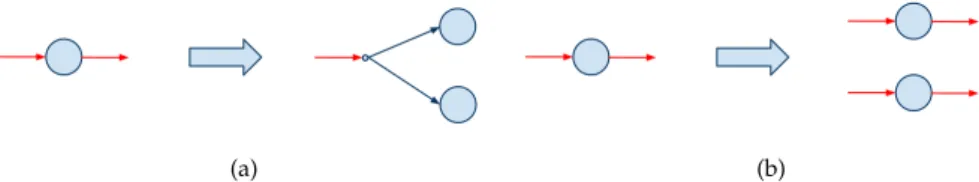
i) Trees: Suppose all objects are put in a single cluster,C₁. A graph

grammar for trees will select a subset of these objects to move to a new clusterC2, and create a branch pointB{C1,C2}that leads toC1andC2, see Fig.3a.

ii) Chains: Suppose, once again, that all objects are put in a single initial clusterC₁. A graph grammar for chains will create a clusterC₂,

and splitC2fromC1. No branchpoint is created in this form, of course, see Fig.3b.

14 the multidimensional road to harvard or, why ranking business schools does not

(a) (b)

Figure3:(a) Tree-generative Graph Operation. (b) Cluster-generative Graph Operation

’splitting’ process to continue until a final structure is reached. Also, items may eventually be moved between clusters, if the model finds that this would create a structure that is more adequate to the data.

We will close our description over the principal points of the original authors’ algorithm by focusing on the process of generating the split space via Stirling Numbers.

2.2.3 Stirling Numbers

As we have mentioned, the KT algorithm chooses, at each iteration, one best split operation to apply over the graph. This requires generating the possibility space of all potential split locations. In order to generate the hypothesis space of possible splits, the Stirling numbers of the second kind are used. A Stirling number is calculated as follows:

S(m,n) = 1 n!

X

(−1)k

n n−k

(n−k)m

This enumerates the ways of distributingmdistinct objects into n

identical containers with no container left empty.

Given this brief summary of KT-Structures, we may now proceed to apply the model to the Business Week Rankings of US-based MBA Programs.

2.3 the business week 2008 ranking

Our first experiment computes KT-Structures of the Business Week2008 ranking. The purpose is to compare and contrast the rankings widely used with the KT-Structure. All the21possible forms provided in the method were computed, and we concentrated attention to those that suggested rank anomalies. Of these, the tree and hierarchy structures readily presented potential rank anomalies, and we concentrate focus on them here.

2.3.1 Materials and Methods

2.3 the business week 2008 ranking 15

a student living in Bloomington IN has the exact same experience of a student living in New York City—the data is simply oblivious to this information). These dimensions are: graduate poll, corporate poll, intellectual capital, tuition and fees, pre-MBA pay, post-MBA pay, selectivity, job offers, general management, analysis, teaching, and careers. These last four dimensions ranged from A+ to C, and we changed these results to numerical values (A+, A, B, and C were translated to1,2,3, and4, respectively).

Notice an important aspect here. The model does not know that an A-grade is better than a C-grade, or that a higher post-MBA pay value is better than a lower one. The method does not have any information concerning the meaning of all these variables. But there are strong rela-tions between the data: ranks are provided by orders; tuition, fees and pay are determined by the market, letter grades are obtained through Business Week’s polls, etc. The model is able to compute the structures based only on the underlying data, and does not need to understand themeaningimbued in each dimension—the problem of meaning is far from solved in cognitive science [Linhares2000,Linhares e Brum2007].

While we did not have access to the original polling data utilized in building the original ranking, the relevance of the questions and issues posed here remain. Because of this, we avoid direct criticism of the methodology and steer away from a direct comparison of our results to those of the publication. For a deeper description of how Business Week built their ranking, please see [Gloeckler et al.2008]

2.3.2 Numerical experiments

The most interesting form is a hierarchy; presented in figure4. At a macro level, this form has some semblance with the original ranking (Figure 5). The KT-Structure distance between two schools (i,j) is

measured by counting the number of edges from the origin school’s cluster to the destination school. The rank distance, on the other hand, is simply obtained by |Ri−Rj|, whereRk is the position of schoolk in the rank. Note that the domains are quite distinct, as distances in the KT-Structure tend to be smaller, yet, there is positive correlation between the rank and the hierarchy (r=.65—and covariance is8.34). This shows that—at a large scale—there is some agreement between the rank and the KT-Structure.

The striking characteristic of trees and hierarchies—as contrasted to rankings—is the possibility of branchpoints. If the reader will allow a metaphor: given the data, schools are better viewed as cities orga-nized alongside a river rather than as elevator stops on a skyscraper. The glacier melts at the left side of fig.4, with the cluster comprising Harvard, Stanford and Wharton. As one moves downstream, the dif-ferentiating variable (at this point) is post-MBA pay: the first cluster with three schools are the only ones over $120k, the second cluster with values ranging from $105k (Chicago) to $116k (MIT). The cluster comprising Michigan ($105k) and Duke ($100k) is followed by one comprising Cornell ($96k) and NYU ($95k). There are three schools downstream with post-MBA pay of $100k or more (UCLA, Virginia, and CMU), but at this stage many other variables become increasingly relevant, and the tree branches.

in "general management" and "analysis" (and B’s in "careers"), they are low-ranked in the corporate poll (positions33,41, and42), and they are relatively expensive. These traits lead us to interesting distortions between this tree and the rankings.

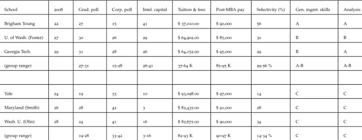
As a demonstration of the explaining power of the KT-Structure, consider the following example. Suppose a student preferred the Uni-versity of Washington’s Foster School (no.27), but was rejected there and accepted by two schools: Yale (no.24) and Georgia Tech (no.29). The student’s choice seems easy, as Yale is no doubt better ranked.

The KT-Structure, however, tells a different story, placing Yale far from the student’s preferred Foster. Here is why. If the student chooses Georgia Tech, tuition costs drop slightly from Foster’s $64,902to Geor-gia Tech’s $64,152—while Yale will charge $93,098. Again, if the student chooses Georgia Tech, Foster’s "B" in "general management" is also found in Georgia Tech—while Yale holds a "C". Finally, if the student chooses Georgia Tech, Foster’s "B" in "analysis" is reflected by an "A" in Georgia Tech’s grade—while Yale holds a "C". Georgia Tech, at the28th position in the corporate poll, is much closer to the preferred Foster’s 26thposition than Yale (33thposition).

Of course, by choosing Yale over Georgia Tech, there are also sig-nificant gains in other dimensions, but these are dimensionswhich the student did not prioritize by choosing Foster. The ranking keeps moving further away from the student’s preferred school characteristics. The preferred school held the30th position in the graduate poll; Georgia Tech holds the 31st—but Yale is at the 19th position. In "intelectual capital", the preferred school held the29thposition, while Georgia Tech holds the26thposition—but Yale is number10. In school selectivity (per-haps a minor concern to our already accepted student), the preferred school accepts 30% of applicants, Georgia Tech accepts29%—while Yale is much more selective, at14%.

Of the12dimensions considered in building the ranking, Yale differs significantly in7dimensions from both the student’s preferred school and from Georgia Tech (and also from Brigham Young). This is why the KT-Structure places schools like Maryland (26) close to Washing-ton University’s Olin (28), while both are far from the University of Washington’s Foster (27) and Georgia Tech (29) (which also resemble each other in many dimensions). Instead of differentiating them, the

School 2008 Grad. poll Corp. poll Intel. capital Tuition & fees Post-MBA pay Selectivity (%) Gen. mgmt. skills Analysis

Brigham Young 22 27 15 41 $37,010.00 $90,000 56 A A

U. of Wash. (Foster) 27 30 26 29 $64,902.00 $85,000 30 B B

Georgia Tech. 29 31 28 26 $64,152.00 $95,000 29 B A

(group range) 27-31 15-28 26-41 37-64K 85-95K 29-56% A-B A-B

Yale 24 19 33 10 $93,098.00 $97,000 14 C C

Maryland (Smith) 26 28 42 3 $82,435.00 $91,000 28 C C

Wash. U. (Olin) 28 24 41 16 $82,672.00 $90,000 34 C C

(group range) 19-28 33-42 3-16 82-93K 90-97K 14-34% C C

Table1:Rank anomalies. Though schools ranked {22,24,26,27,28, and29} seem

close in the ranking, they are clearly separable into different clusters.

Figure4:The generated KT-Structure: an undirected hierarchy with no self-links.

Figure5:The KT-Structure distance between schools plotted against their ranked distance.

rank alternates between these two different groups, obliterating their differences along the way. These are serious rank anomalies.

In sum: if the ontology of the world of MBA programs consisted solely of the12 dimensions included in the rankings, which is ques-tionable, and if the collected data were an absolutely perfect reflection of reality, which is also questionable, and even if the aforementioned criticisms of rankings brought forth in the literature were all invalid, which also happens to be questionable, this much is true: a student with a strong preference for the no.27th school would find that school no.29seems a better match than school no.24. If, in an ideal world, popular publications provided other visualizations instead of rankings, there would be no cognitive dissonance in choosing between a school that better reflects one’s true preferences versus the "better ranked" one. (We in fact hypothesize that students facing these choices would choose schools according to the KT-Structure more often than according to rank, though we have no way to test this at this point). This is the type of meaningful information which the KT-Structure brings to light and to which a simple rank ordering remains oblivious.

The KT-Structure enables a comparison to other schools in the same cluster and, moreover, highlights the differences between the clusters upstream. A school can move faster if it knows exactly where it is located in this multidimensional space, and sensitivity analysis can be conducted through careful variations of parameters. There are no sudden jumps here; as there are many multidimensional curves on the road to Harvard1_.

2.4 summary

We introduce to the decision science community, Kemp and Tenen-baum’s model for finding structure in data. Instead of presenting it under the perspective of a psychological theory, our goal here is to describe it as a new methodology for research. In our experiments, we

1 Harvard is not used here to express endorsement or any other value judgment. Because

of its great wealth, history, faculty, and alumni, it can be argued that Harvard University— and HBS—has become the archetype of the "world-class" University.

have applied the method to the data used to construct school rankings by Business Week (2008). We claim the method provides insights into the multidimensional space in which schools compete, and that the re-sulting KT-Structures better reflect the multi-faceted reality of business schools and are better representations than the widely disseminated rankings.

Using the very same features used by Business Week, the KT-Structures bring to light anomalies in which schools may be next to each other in the rankings while bearing few resemblances in their numerous dimensions. Conversely, schools can be far in the rankings, but have a large set of similar features. We therefore question the validity of school rankings: A rank is not necessarily the most adequate form to represent (or understand) entities with no dominance relation. Statistical and data mining methods often pressupose a hidden structure, such as a cluster, a tree, or a ranking. The MBA program rankings, however, impose a representational form that is unfit for the type of information they hope to convey. This has sweeping implications to school strategy, positioning, and, because of the wide impact of published rankings, for prospective students and all stakeholders. One can only idealize a world in which the structures that best reflect the data are widely disseminated for public consumption. We hope readers will receive this introduction to KT-Structures with the recognition that this is an innovative, promising approach that deserves to be admitted into the decision scientist’s toolbox of research methods.

Part III

3

O N A S PA R S E D I S T R I B U T E D M E M O RY

In order to more fully understand this reality, we must take into account other dimensions of a broader reality. — John Archibald Wheeler (1911-2008)

3.1 introduction

Human short-term memory is severely limited. While the existence of such limits is undisputed, there is ample debate concerning their nature. Miller [Miller1955] described the ability to increase storage capacity by grouping items, or “chunking”. He argued that the span of attention could comprehend somewhere around seven information items. Chunk structure is recursive; as chunks may contain other chunks as items: Paragraphs built out of phrases built out of words built out of letters built out of strokes. This mechanism is used to explain the cognitive capacity to store a seemingly endless flux of incoming, pre-registered, information, while remaining unable to absorb and process new (non-registered) information in highly parallel fashion.

Miller’s ‘magic number seven’ has been subject of much debate over the decades. Some cognitive scientists have modeled such limits by sim-ply using (computer-science) “pointers”, or “slots” [Gobet e Simon2000,

Gobet et al.2001]—see [Linhares e Brum2007,Linhares e Freitas2010] for debate. However, such approaches do not seem plausible given the massively parallel nature of the brain, and we believe memory limits are an emergent property of the neural architecture of the human brain. As Hofstadter put it a quarter of a century ago [Hofstadter1985, p.

642]: the “problem with this [slot] approach is that it takes something that clearly is a very complex consequence of underlying mechanisms and simply plugs it in a complex structure, bypassing the question of what those underlying mechanisms might be”.

Our objective in this chapter is to study these memory limits as emer-gent effects of underlying mechanisms. We postulate two mechanisms, discussed in previous literature. The first is a mathematical model of human memory brought forth by Kanerva [Kanerva1988], called Sparse Distributed Memory (SDM). We also presuppose, following [Kanerva1993], an underlying mechanism of chunking through averag-ing. It is not within the scope of this study to argue the validity of SDM as a cognitive model. For incursions on this broader topic, we direct the reader to [Kanerva1993, Stewart e Eliasmith2009, Gayler2003] who discuss the plausibility of this Vector Symbolic Architecture family of models (in which SDM is contained).

This work, while similar in its mathematical foundations, is differ-ent from previous capacity analyses: In [Kanerva1988], the memory capacity analysis relates to long-term memory mechanisms, while we study the short-term memory limits (of this same model). Our work also differs from that of Plate, in that, regardless of the number of items presented, the memory will only store (and subsequently retrieve) a

psychologically plausible number of items. The difference becomes salient in Plate’s own description [Plate2003, p.139]: “As more items and bindings are stored in a single HRR the noise on extracted items increases. If too many associations are stored, the quality will be so low that the extracted items will be easily confused with similar items or, in extreme cases, completely unrecognizable".

A number of theoretical observations are drawn from our computa-tions: i) a range of plausible numbers for the dimensions of the memory, ii) a minimization of a current controversy between different ‘magic number’ estimates, and iii) potential empirical tests of the averaging assumption. We should start with a brief description of our postulates: i) the SDM, and ii) chunking through averaging.

3.1.1 Sparse Distributed Memory

The Sparse Distributed Memory (SDM), developed in [Kanerva1988], defines a memory model in which data is stored in distributed fashion, in a vast, sparsely populated binary address space. In this model, (a number of) neurons act asaddress decoders. Consider the space{0,1}N: SDM’s address space is defined allowing2Npossible locations, where Ndefines both the word length and the number of dimensions of the

space (e.g., the memory holds binary vectors of lengthN). In SDM, the data is the same as the medium in which it is stored (i.e. the stored items areN-bit vectors inN-dimensional binary addresses).

SDM uses Hamming distance as a metric between any twoN-bit

vec-tors (hereafter memory items, items, elements, or bitstrings—according to context). Neurons, orhard locations(see below), in Kanerva’s model, hold random bitstrings with equal probability of0’s and1’s—Kanerva [Kanerva1994, Kanerva2009] has been exploring a variation of this model with a very large number of dimensions (around10000). (With the purpose of encoding concepts at many levels, the Binary Spatter Code—or BSC—, also shares many properties with SDM.)With the Hamming distance as a metric, one can readily see that the average distance between any two points in the space is given by the binomial distribution, and approximated by a normal curve with mean atN/2

with standard deviation√N/2. Given the Hamming distance, and large N, most of the space lies close to the mean. A low Hamming distance

between any two items means that these memory items are associated. A distance that is close to the meanN/2means that the memory items

are orthogonal to each other. This reflects two facts about the organiza-tion of human memory: orthogonality of random concepts, and close paths between random concepts.

Orthogonality of random concepts: the vast majority of concepts is or-thogonal to all others. Consider a non-scientific survey during a cogni-tive science seminar, where students asked to mention ideas unrelated to the course brought up terms like birthdays, boots, dinosaurs, fever, executive order, x-rays, and so on. Not only are the items unrelated to cognitive science, the topic of the seminar, but they are also unrelated to each other.

Close paths between concepts: The organization of concepts seems to present a ’small world’ topology–for an empirical approach on words, for instance, see [Cancho e Solé2001]. For any two memory items, one can readily find a stream of thought relating two such items (‘Darwin gavedinosaurstheboot’; ‘she ran afeveron herbirthday’; ‘isn’t it time for

the Supreme Court tox-raythatexecutive order?’ . . . and so forth). Robert French presents an intriguing example in which one suddenly creates a representation linking the otherwise unrelated concepts of ’coffee cups’ and ’old elephants’ [French1997]. In sparse distributed memory, any two bitstrings with Hamming distance aroundN/4would be extremely

close, given the aforementioned distribution. AndN/4is the expected

distance of an average point between two random bitstrings.

Of course, for largeN(such asN>100), it is impossible to store all

(or even most) of the space—the universe is estimated to carry a storage capacity of 1090 bits (10120 bits if one considers quantum gravity)

[Lloyd2002]. It is here that Kanerva’s insights concerning sparseness and distributed storage and retrieval come into play:220_{—or a number} around one million–physical memory locations, called hard locations, could enable the representation of a large number of different bitstrings. Items of a large space with, say,21000locations would be stored in a

mere220hard locations—the memory is indeed sparse.

In this model, every single item is stored in several hard locations, and can, likewise, be retrieved in distributed fashion. Storage occurs by distributing the item in every hard location within a certain threshold ‘radius’ given by the Hamming distance between the item’s address and the associated hard locations. Different threshold values for differ-ent numbers of dimensions are used (in his examples, Kanerva used 100,1000 and10000dimensions). ForN =1000, the distance from a

random point of the space to its nearest (out of the one million) hard locations will be approximately424bits [Kanerva1988, p.56]. In this scenario, a threshold radius of451bits will define anaccess sphere con-taining around 1000 hard locations. In other words, from any point of the space, approximately 1000 hard locations lie within a 451-bit distance. All of these accessible hard locations will be used in storing and retrieving items from memory. We therefore define the function

A:{0,1}N×{1,2,. . .,N}7→2{0,1}Nand a hard locationψx∈A(x,R)iff

ψx∈{0,1}N∧H(x,ψx)6R, whereAdefines an access radius around

xof sizeR(451ifN=1000;His the Hamming distance).

A brief example of a storage and retrieval procedure in SDM is in order: to store an item xat a given (virtual) location ζ(in sparse

memory) one must activate every hard location within the access sphere ofxand store the datum in each one. Hard locations carryNadders, one

for each dimension. To store a bitstringxat a hard locationψ, one must

iterate through the adders ofψ: If theith bit ofxis1, increment theith

adder ofψ, if it is0, decrement it. Repeating this for all hard locations inx’s access sphere will distribute the information inxthroughout the

hard locations.

Retrieval of data in SDM is also massively collective and distributed: to peek the contents of each hard location, one computes its related bit vector from its adders, assigning theith bit ofψas a1or0if thei-th

adder is positive or negative, respectively (a coin is flipped if it is0). Notice, however, that this information in itself is meaningless and may not correspond to any one specific datum previously registered. To read from a locationxin the{0,1}Naddress space, one must activate the hard locations in the access sphere ofxand gather each related bit vector.

The stored datum will be the majority rule decision of all activated hard locations’ related bit vectors. If, for the ith bit, the majority of all bit vectors is1, the final read datum’sithbit is set to1, otherwise to0. Thus, “SDM is distributed in that many hard locations participate in storing

and retrieving each datum, and one hard location can be involved in the storage and retrieval of many data” [Anwar e Franklin2003, p.342].

All hard locations within an access radius collectively point to an address. Note also that this process is iterative. The address obtained may not have information stored on it, but it provides a new access radius to (possibly) converge to the desired original address. One par-ticularly impressive characteristic of the model is its ability to simulate the ´tip-of-tongue´ phenomenon, in which one is certain about some features of the desired memory item, yet has difficulty in retrieving it (sometimes being unable to do so). If the requested address is far enough from the original item (209bits ifN=1000), iterations of the

process will not decrease the distance—and time to convergence goes to infinity.

The model is robust against errors for at least two reasons: i) the contribution of any one hard location, in isolation, is negligible, and ii) the system can readily deal with incomplete information and still converge to a previously registered memory item. The model’s sparse nature dictates that any point of the space may be used as a storage address, whether or not it corresponds to a hard location. By using about one million hard locations, the memory’s distributed nature can ‘virtualize’ the large address space. The distributed aspect of the model allows such a virtualization. Kanerva [Kanerva1988] also discusses the biological plausibility of the model, as the linear threshold function given by the access radius can be readily computed by neurons, and he suggests the interpretation of some particular types of neurons as address decoders. Given these preliminaries concerning the Sparse Distributed Memory, we should now proceed to our second premise: chunking through averaging.

3.1.2 Chunking through averaging

To chunk items, the majority rule is applied to each bit: givenvbitstrings

to be chunked, for each of theNbits, if the majority is1, the resulting bitstring’s chunk bit is set to1; otherwise it is0. In case of perfect ties (no majority), a coin is flipped.

We have chosen the term ’chunking’ to describe an averaging opera-tion, and ’chunk’ to describe the resulting bitstring, because, through this operation, the original components generate a new one to be written to memory. The reader should note, in SDM’s family of high-dimensional vector models, called Vector Symbolic Architectures (VSA), the operation that generates composite structures is commonly known as superposition [Stewart e Eliasmith2009,Gayler2003,Plate2003].

Obviously, this new chunked bitstring may be closer, in terms of Hamming distance, to the original elements, than the mean distance

N/2between random elements (500bits ifN=1000), given a relatively smallv. The chunk may then be stored in the memory, and it may be used in future chunking operations, allowing, thus, for recursive behav-ior. Let us denote this averaged bitstring asα. With these preliminaries,

we may turn to numerical results.

3.2 analysis

3.2.1 Computing the Hamming distance from chunkαto items

Let ξ = {ξ1,ξ2, ...,ξv} be the set of bitstrings to be chunked into a new bitstring, α. The first task is to find out how the Hamming

distance is distributed between this averagedαbitstring and the set

ξ = {ξ1,ξ2, ...,ξv} of bitstrings being chunked. This is, as discussed, accomplished through majority rule at each bit position. Imagine that, for each separate dimension, a supreme court will cast a decision with each judge choosing yes (1) or no (0). If there is an even number of judges, a fair coin will be flipped in the case of a tie. Given that there arev=|ξ|votes cast, how many of these votes will fall in the minority side? (Each minority-side vote adds to the Hamming distance between an itemξi and the averageα.)

Note that the minimum possible number ofminority votesis one, and that it may occur with either3votes cast or two votes and a coin flip. If there are two minority votes, they may stem from either5votes or 4votes and a coin flip, and so forth. We thus have that, for v votes,

the maximum minority number is given by⌊v/2_⌋(and the ambiguities

between an odd number of votes versus an even number of votes plus a coin flip are resolved by considering2⌊v/2⌋+1total votes). This leads

to independent Bernoulli trials, with success factorp= 1/2, and the

constraint that the minority view differs from the majority bit vote. Let

Xbe a random variable with the number of minority votes. Obviously

in this case,P(16X6_⌊v/2_⌋) =P(X6_⌊v/2_⌋−1), hence we have, forv

items, the following cumulative distribution function of minority votes [Boland1989]:

P(X6_⌊v/2_⌋−1) =

⌊v/2⌋−1

X

i=0

2_⌊v/2_⌋ i

pi(1−p)2⌊v/2⌋−i=

=

⌊v/2⌋−1

X

i=0

(2_⌊v/2⌋)!

i!(2_⌊v/2_⌋−i)! 1 2

2⌊v/2⌋

=4−⌊v/2⌋

⌊v/2⌋−1

X

i=0

(2_⌊v/2⌋)!

i!(2_⌊v/2_⌋−i)!

While we can now, given v votes, compute the distribution of

mi-nority votes, the objective is not to understand the behavior of these minority bitsin isolation, i.e., per dimension on the chunking process. We want to compute the number of dimensions to (in a psychologi-cally and neurologipsychologi-cally plausible way) store and retrieve aroundM

items—Miller’s number of retrievable elements—through an averaging operation. Hence we need to compute the following:

(I) Given a number of dimensionsNand a setξof items, the

probability density function of the Hamming distance from

αto the chunked elementsξ_i,

(II) A threshold T: a number of dimensions in which, if an

elementξi’s Hamming distance toαis farther from that point, thenξicannot be retrieved,

(III) As|ξ|grows, how many elements remain retrievable?

N TN,2σ(M=4or5) TN,2σ(intermediary value) TN,2σ(M=6or7)

64 27.42 28.51 29.6

128 50.49 52.62 54.75

192 72.85 76.01 79.16

256 94.83 99.02 103.2

320 116.58 121.8 126.99

384 138.17 144.4 150.61

448 159.62 166.88 174.11

512 180.98 189.25 197.49

576 202.25 211.54 220.8

640 223.45 233.76 244.03

704 244.6 255.92 267.2

768 265.69 278.02 290.32

832 286.74 300.09 313.4

896 307.75 322.11 336.43

960 328.72 344.1 359.43

1024 349.66 366.05 382.4

100 40.52 42.2 43.87

1000 341.82 357.82 373.79

10000 3217.7 3375.16 3532.49

Table2:Thresholds TN,2σgiven plausible success factors and dimension combinations.

Given bitstrings with dimension N, suppose v = |ξ| elements have been chunked, generating a new bitstring α. Let HN(α,ξi) be the Hamming distance from the chunked elementαtoξi, theith element ofξ. What is the distance fromαto elements inξ? Here we are led to

NBernoulli trials with success factorp_|ξ|. SinceNis large,H_N(α,ξ_i)

fori={1,2,. . .,v}can be approximated by a Normal distribution, we may useµ=Np_|ξ| andσ=qNp_|ξ|(1−p_|ξ|). To model human short

term memory’s limitations, we want to compute a cutoff thresholdTN which will guarantee retrieval of aroundMitems averaged inαand “forget” itemsξ_iifH_N(α,ξ_i)> T_N—whereMis the Miller’s limiting

number. Hence to guarantee retrieval of around95% (2σ) ofMitems,

we haveTN,2σ=NpM+2

p

NpM(1−pM), wherepMis the success factor corresponding toM. Note that Cowan [Cowan2000] has argued for a “magic number” estimate of4±1items—and the exact cognitive limit is still a matter of debate. The success factor for4(or5) elements isp_{4,5}=.3125; and for6(or7) elements it isp_{6,7}=.34375. By fixing the success factor at plausible values ofM({4,5}, or an intermediary value between {4,5} and {6,7}, or {6,7}), different threshold valuesTN,2σare obtained for varyingN, as shown in Table2. In the remainder of this study, we use the intermediary success factorpM=.328125=21/64for our computations; again without loss of generality between different estimates ofM.

We thus have a number of plausible thresholds and dimensions. We can now proceed to compute the plausibility range: Despite the

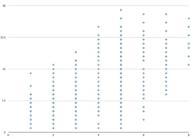
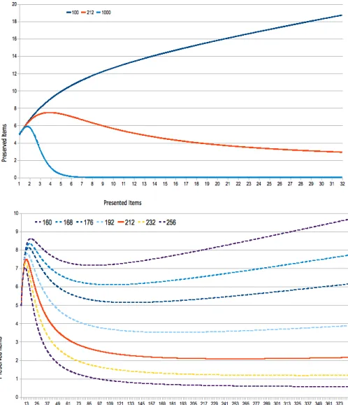
Figure6:Behavior at different dimensions and items presented

implicit suggestion in Table1that any number of dimensions might be plausible, how does the behavior of these(N,T_N,2σ)combinations vary as a function of the number of presented elements,|ξ|?

3.2.2 Varying the number of presented items

Consider the case of information overload, when one is presented with a large set of items. Suppose one were faced with dozens, or hundreds, of distinct items. It is not psychologically plausible that a large number of elements should be retrievable. For an itemξito be impossible to retrieve, the distance between the averaged item α and ξi must be higher than the threshold point of the correspondingN. When we have an increasingly larger set of presented items, there will be information loss in the chunking mechanism, but it should still be possible to retrieve some elements within plausible psychological bounds.

Figure1(a) shows the behavior of three representative sizes ofN:100, 212 and1000 dimensions. (100and1000 were chosen because these

are described in Kanerva’s original examples of SDM.)N = 212 has shown to be the most plausible number of dimensions, preserving a psychologically plausible number of items after presentations of different set sizes. It is clear thatN=100quickly diverges, retaining

a high number of items in a chunk (as the number of presented items grows). Conversely, if N = 1000, the number of preserved memory

items rapidly drops to zero, and the postulated mechanisms are unable to retrieve any items at all—a psychologically implausible development. Figure1(b) zooms in to illustrate behavior over a narrower range of

N-values and a wider range of presented items. Varying the number

of presented items and computing the number of preserved items (for a number of representative dimensions) yields informative results. Based on our premises, experiments show that to appropriately reflect the storage capacity limits exhibited by humans, certain ranges ofN

must be discarded. With too small a number of dimensions, the model will retrieve too many items in a chunk. With too large a number of dimensions, the model will retrieve at most one or two—perhaps no items at all. This is because of the higher number of standard deviations involved in the dimension sizes: for N = 100, the whole

space has20 standard deviations, andTN=100,2σ = 42.2 is less than 2standard deviations below the mean—which explains why an ever growing number of items is “retrieved” (e.g., high probability of false positives). ForN = 1000, the space has over63 standard deviations, andT_N=1000,2σ=357.82, is around8.99standard deviations below the mean. There is such a minute part of the space belowT_N=1000,2σthat

item retrieval is virtually impossible.

With an intermediary success factorpMbetweenp4 andp7 estab-lished by the cognitive limits4and7, we have computed the number of dimensions of a SDM as lying in the vicinity of212dimensions. Variance is minimized whenN=212—and retrieval results hold psychologically plausible ranges even when hundreds of items are presented (i.e., the SDM would be able to retrieve from a chunk no more than nine items and at least one or two, regardless of how many items are presented simultaneously). Finally, given that this work rests upon the chunking through averaging postulate, in the next section we will argue that the postulated mechanism is not only plausible, but also empirically testable.

3.2.3 The chunking through averaging postulate

Consider the assumption of chunking through averaging. We propose that it is plausible and worthy of further investigation, for three reasons.

This assumption minimizes the current controversy between Miller’s estimations and Cowan’s. The disparity between Miller’s7±2or Cowan’s 4±1observed limits may be a smaller delta than what is argued by Cowan. Our ‘chunking-through-averaging’ premise may provide a sim-pler, and perhaps unifying, position to this debate. If chunking4items has the same probability as5items, and chunking6items is equivalent to chunking7items, one may find that the ‘magic number’ constitutes one cumulative probability degree (say,4-or-5items) plus or minus one (6-or-7items).

A mainstream interpretation of the above phenomenon may be that, as with any model, SDM is a simplification; an idealized approximation of a presumed reality. Thus, one may see it as insufficiently complete

to accurately replicate the details of true biological function due to, among other phenomena, inherent noise and spiking neural activity. In this case, one would interpret it as a weakness, or an inaccuracy inherent to the model. An alternative view, however improbable, may be that the model is accurate in this particular aspect, in which case, the assumption minimizes the current controversy between Miller’s estimations and Cowan’s.

The success factors computed above show that for either4or5items, we havep= .3125, while for6or 7items we havep = .34375. If we

assume an intermediary value ofp—which is reasonable, due to noise

or lack of synchronicity in neural processing [Borisyuk et al.2000]—the controversy vanishes. We chose to base our experiments on the inter-mediary average value (p=21/64= .328125), and the results herein may be adapted to other estimates as additional experiments settle the debate.

Moreover, a chunkαtends to be closer to theξichunked items than these items are between themselves. For example, with |ξ| = 5 and N=212, the Hamming distance between a chunk and a random item is drawn from a distribution withµ=N21/64andσ= (√N√903)/64;

in here, from the point of view of the chunked itemα, the closest1% of the space lies at53bits, while99% of the space lies at84bits. Contrast this with the distances between any two random, orthogonal, items, which are drawn fromµ=N/2andσ=√N/2: from the point of view

of a random item, the closest 1% of the space lies at 89 bits, while 99% of the space lies at122. This disparity reflects the principles of orthogonality between random conceptsand ofclose paths between concepts (or small worlds [Cancho e Solé2001]):the distance between2items from any 5is large, but the distance to the average of the set is small. Of course, as|ξ|grows, the distance toαalso grows (since lim|ξ|→_∞p|ξ|=

1/2), and items become irretrievable. One thing is clear: with5chunked items, the chance of retrieving a false positive is minute.

Finally, the assumption of chunking through averaging is empirically testable. Psychological experiments concerning the difference in ability to retain items could test this postulate. The assumption predicts that (4,5) items, or more generally that (2v,2v+1) for integerv > 0will be

registered with equal probability. It also predicts how the probability of2v+2retained items should drop in relation to2v+1ifv > 0. This

is counterintuitive and can be measured experimentally. Note, however, two qualifications: first, as chunks are hierarchically organized, these effects may be hard to perceive in experimental settings. One would have to devise an experimental setting with assurances that only chunks from the same level are retrievable–neither combinations of such chunks, nor combinations of their constituting parts. The final qualification is that, asvgrows, the aforementioned probability difference tends to zero.

Because of the conjunction of these qualifications, this effect would be hard to perceive on normal human behavior.

3.3 discussion

Numerous cognitive scientists model the limits of human short-term memory through explicit “pointers” or “slots”. In this chapter we have considered the consequences of a short-term memory limit given the mechanisms of i) Kanerva’s Sparse Distributed Memory, and ii) chunk-ing through averagchunk-ing. Given an appropriate choice for the number of